
Analysis of Two-Dimensional Hydraulic Characteristics of Vertical-Slot, Double-Pool Fishway Based on Fluent
Abstract
:1. Introduction
2. Materials and Methods
2.1. Numerical Framework
2.2. Mathematical Model
2.2.1. Model Development
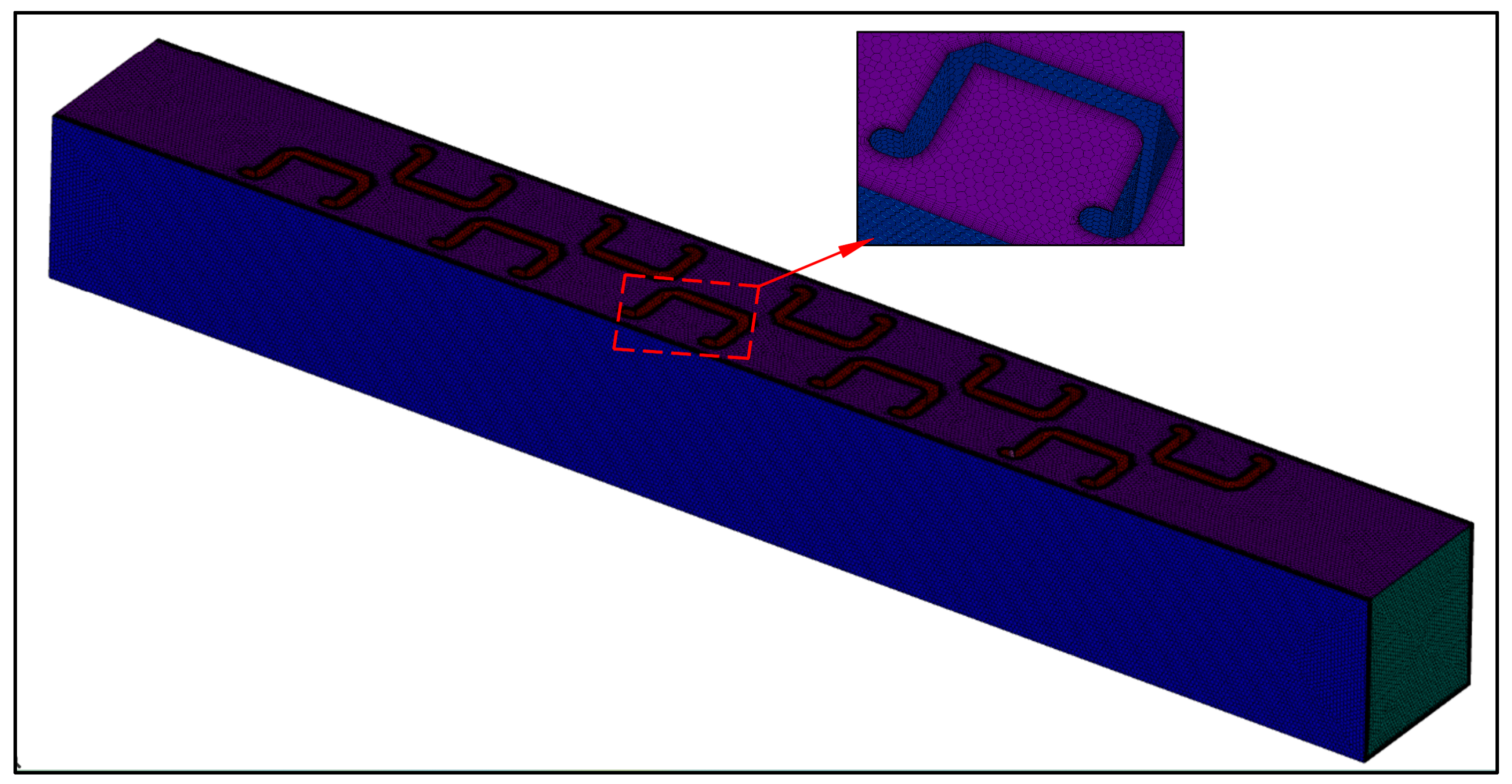
2.2.2. Meshing and Boundary Conditions
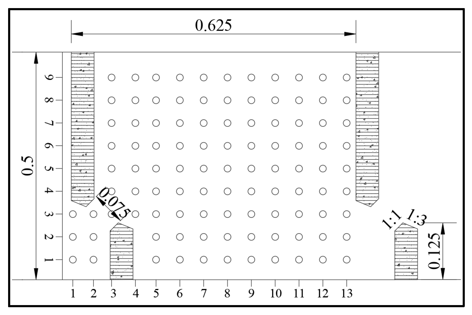
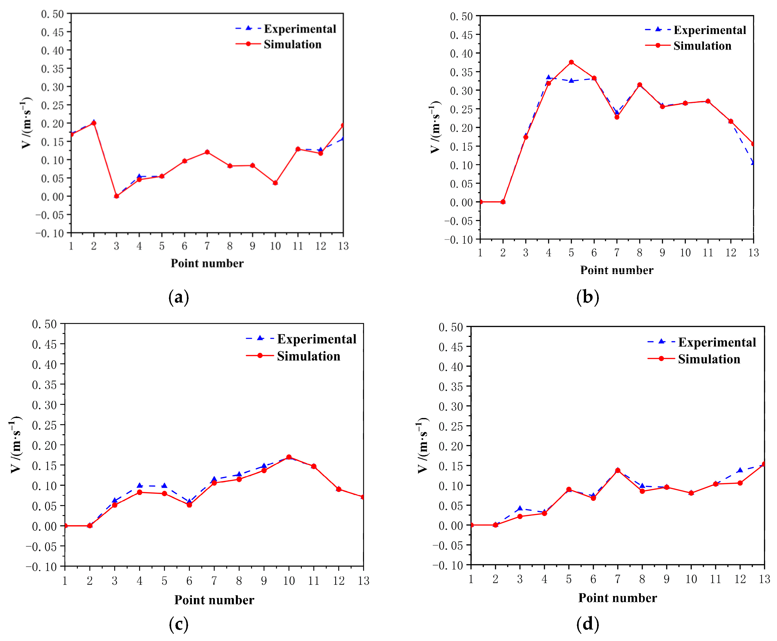
2.3. Model Validation
3. Results and Discussion
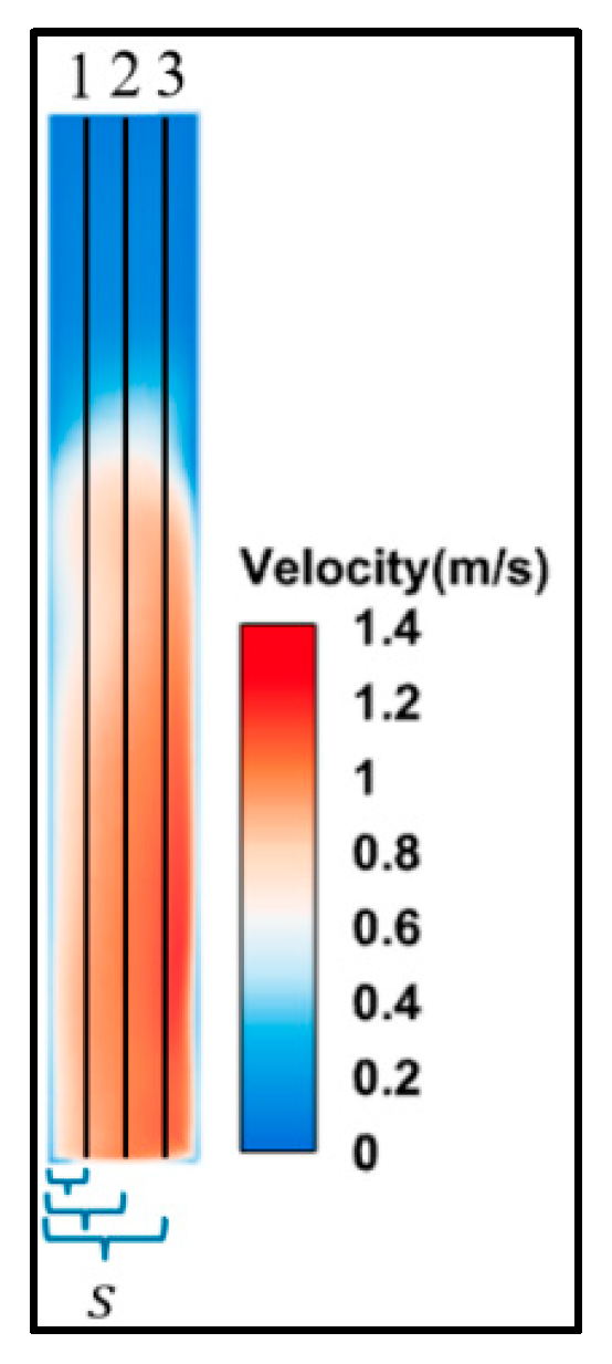
3.1. Flow Field Distribution at the Vertical Slot
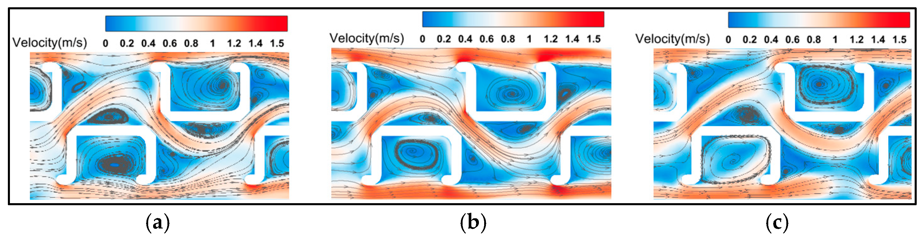
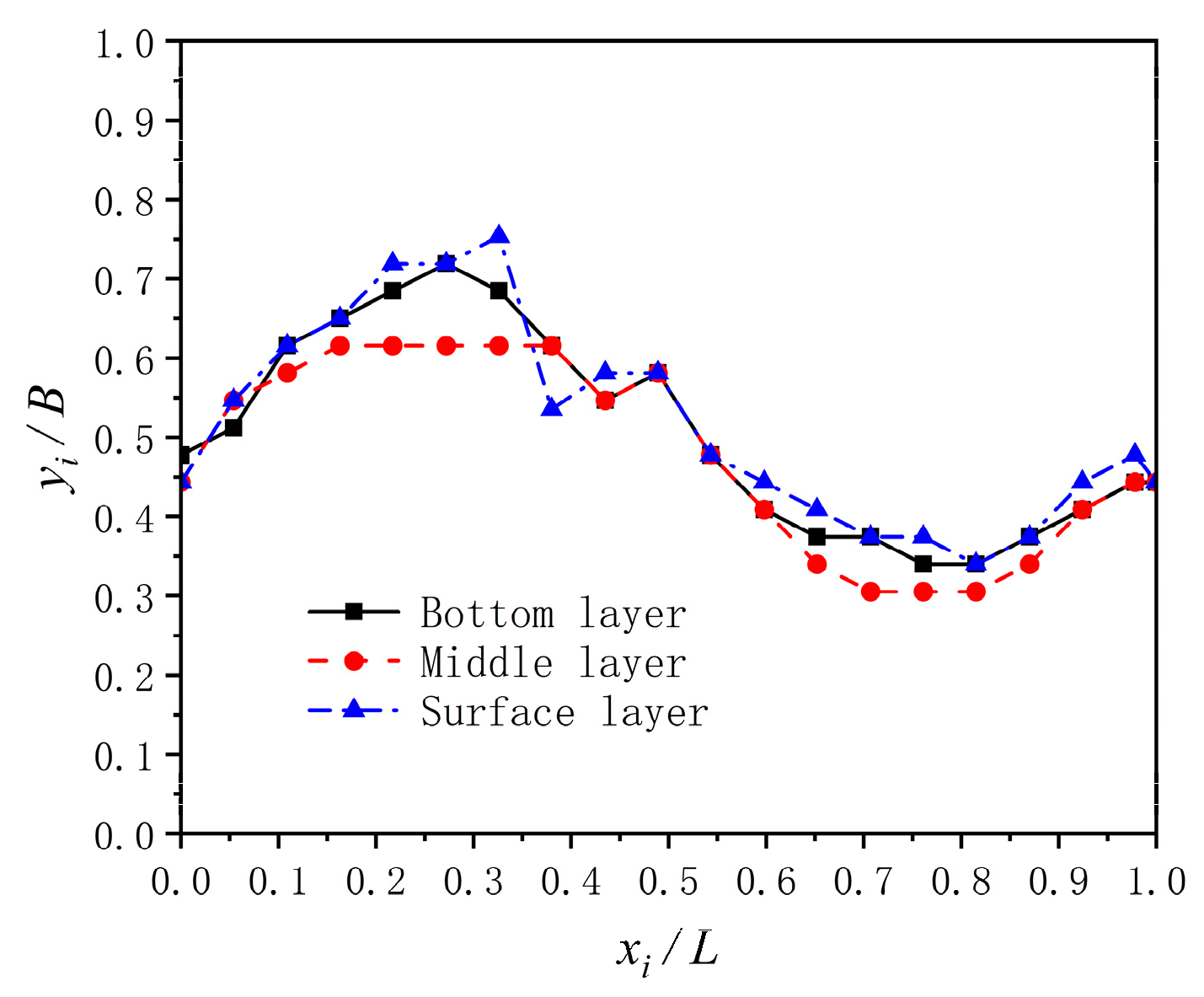
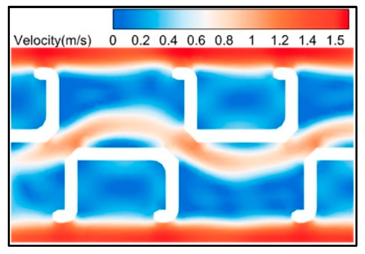
3.2. Calculation Results of the Mainstream Flow Field
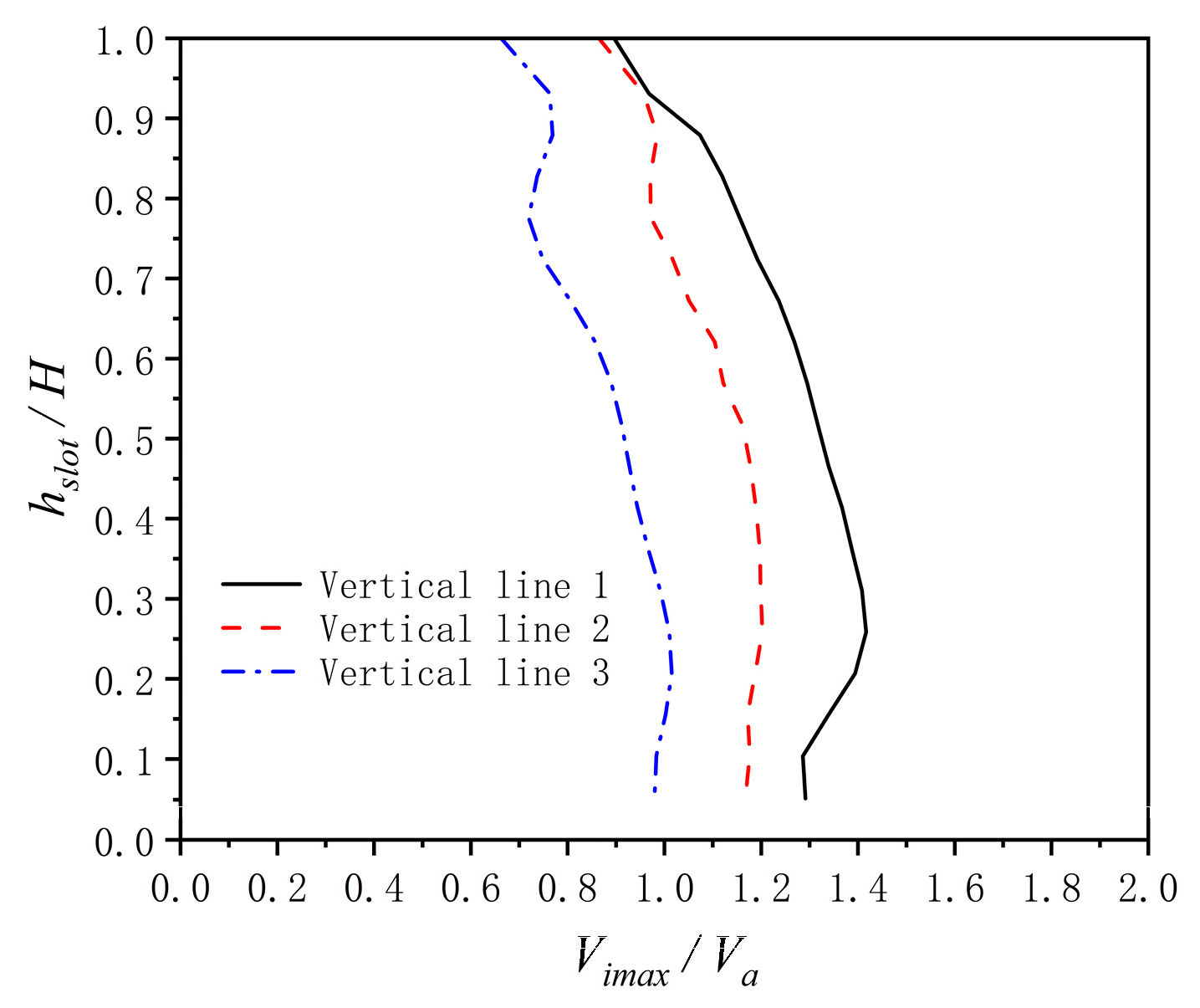
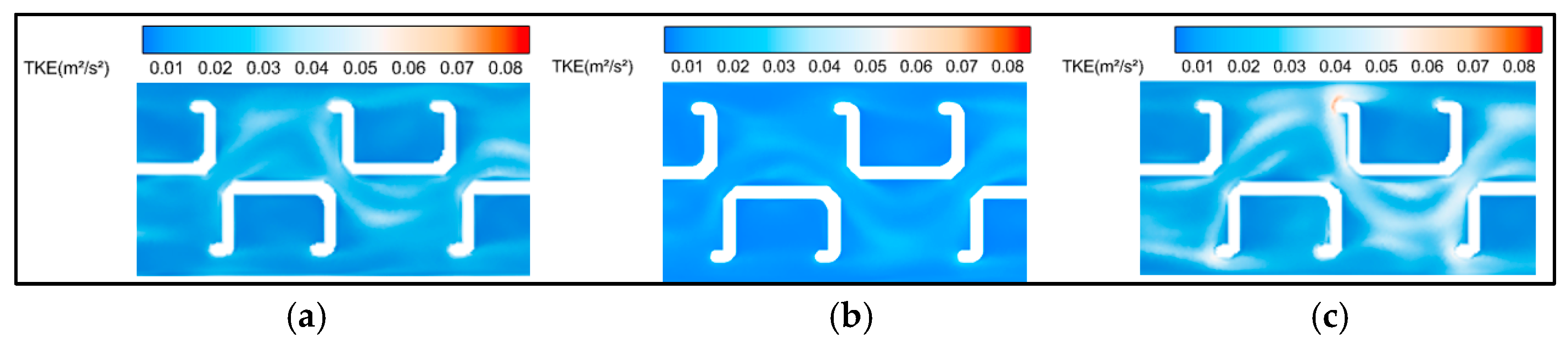
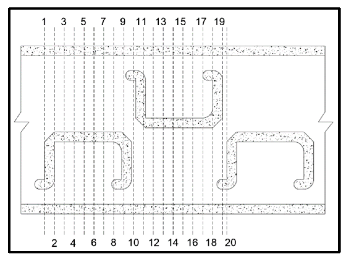
3.3. Analysis of Vertical Flow Field Hydraulic Characteristics
3.4. Comparative Analysis of 3D and 2D Hydraulic Characteristics
4. Conclusions
Author Contributions
Funding
Data Availability Statement
Conflicts of Interest
Abbreviations
| C | The total length of the fishway |
| B | The total width of the fishway |
| L | The length of the unit pool |
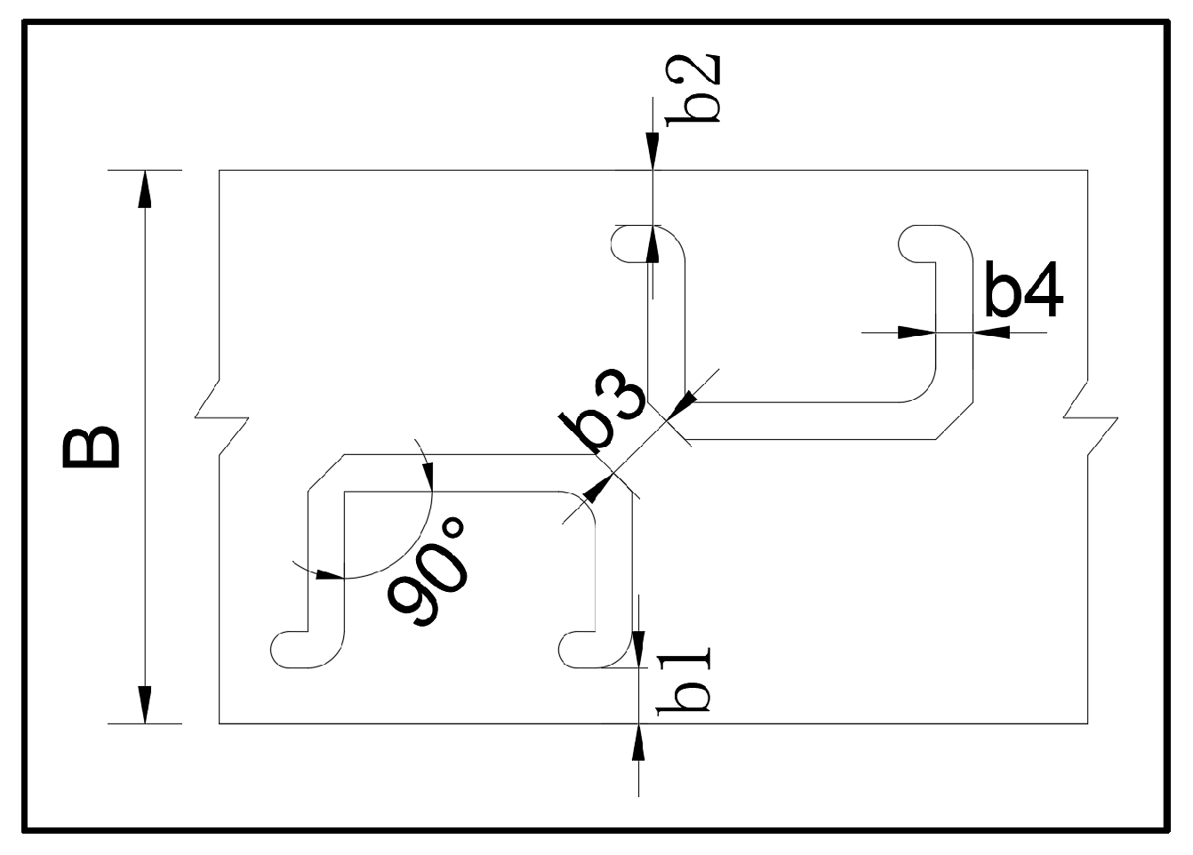
| b1, b2 | The side vertical slots of the fishway |
| b3 | The intermediate vertical slot |
| b4 | Width of the partition in the fishway |
| S | The relative distances of the vertical lines from the left edge along the width direction of the vertical slot |
| Va | Average flow velocity of the vertical slot section |
| Vimax | The maximum flow velocity value on the cross-sectional line |
| hslot | The height of the target from the bottom plate |
| H | Designed water depth |
| W | Vertical flow velocity at the monitoring point |
References
- Chen, S.; Chen, B.; Fath, D.B. Assessing the cumulative environmental impact of hydropower construction on river systems based on energy network model. Renew. Sustain. Energy Rev. 2015, 42, 78–92. [Google Scholar] [CrossRef]
- Kuriqi, A.; Pinheiro, N.A.; Sordo-Ward, A.; Garrote, L. Influence of hydrologically based environmental flow methods on flow alteration and energy production in a run-of-river hydropower plant. J. Clean. Prod. 2019, 232, 1028–1042. [Google Scholar] [CrossRef]
- Ward, J.V. The Four-Dimensional Nature of Lotic Ecosystems. J. N. Am. Benthol. Soc. 1989, 8, 2–8. [Google Scholar] [CrossRef]
- Wang, H.; Wang, C.; Liu, D.; Li, W.; Tong, D. Numerical Simulation Study on Hydraulic Characteristics of Fishway with Cross Partition. Water Resour. Power 2012, 30, 65–68. [Google Scholar]
- Shi, K.; Li, G.; Liu, S.; Sun, S. Experimental study on the passage behavior of juvenile Schizothorax prenanti by configuring local colors in the vertical slot fishways. Sci. Total Environ. 2022, 843, 156989. [Google Scholar] [CrossRef]
- Ahmadi, M.; Kuriqi, A.; Nezhad, H.M.; Ghaderi, A.; Mohammadi, M. Innovative configuration of vertical slot fishway to enhance fish swimming conditions. J. Hydrodyn. 2022, 34, 917–933. [Google Scholar] [CrossRef]
- Santos, J.M.; Silva, A.; Katopodis, C.; Pinheiro, P.; Pinheiro, A.; Bochechas, J.; Ferreira, M.T. Ecohydraulics of pool-type fishways: Getting past the barriers. Ecol. Eng. 2011, 48, 38–50. [Google Scholar] [CrossRef]
- Zheng, T.; Niu, Z.; Sun, S.; Shi, J.; Liu, H.; Li, G. Comparative Study on the Hydraulic Characteristics of Nature-Like Fishways. Water 2020, 12, 955. [Google Scholar] [CrossRef]
- Shen, C.; Yang, R.; Wang, M.; He, S.; Qing, S. Application of Vortex Identification Methods in Vertical Slit Fishways. Water 2023, 15, 2053. [Google Scholar] [CrossRef]
- Ahmadi, M.; Ghaderi, A.; MohammadNezhad, H.; Kuriqi, A.; Di Francesco, S. Numerical investigation of hydraulics in a vertical slot fishway with upgraded configurations. Water 2021, 13, 2711. [Google Scholar] [CrossRef]
- Bombač, M.; Četina, M.; Novak, G. Study on flow characteristics in vertical slot fishways regarding slot layout optimization. Ecol. Eng. 2017, 107, 126–136. [Google Scholar] [CrossRef]
- Barton, A.F.; Keller, R.J. 3D Free surface model for a vertical slot fishway. In Land Waters: Research, Engineering and Man-Agement v.2. Department of Civil Engineering; Monash University: Clayton, Australia, 2003. [Google Scholar]
- Wu, S.; Rajaratnam, N.; Katopodis, C. Structure of flow in vertical slot fishway. J. Hydraul. Eng. 1999, 125, 351–360. [Google Scholar] [CrossRef]
- Bian, Y.; Sun, S. Study on Hydraulic Characteristics of Vertical Slot Fishway. J. Hydraul. Eng. 2013, 44, 1462–1467. [Google Scholar]
- Wang, X.; Zhang, G.; Gao, M.; Ji, X. Numerical Simulation of Hydraulic Characteristics of a New Type of Spiral Fishway. Yellow River 2014, 36, 118–121. [Google Scholar]
- Li, H.; Wang, X.; Zheng, F. Analysis of Three-Dimensional Flow Characteristics in Trapezoidal Fishway. J. Hohai Univ. 2023, 51, 61–65+76. [Google Scholar]
- Ma, W.; Liang, Y.; Wang, M.; Feng, M. Study on hydraulic characteristics of vertical slot-surface orifice combined ecological fishway. Water Resour. Hydropower Eng. 2020, 51, 122–129. [Google Scholar] [CrossRef]
- Nassiraei, H.; Heidarzadeh, M.; Shafieefar, M. Numerical simulation of long waves (tsunami) forces on caisson breakwaters. Sharif Civil Eng. 2016, 32, 3–12. [Google Scholar]
- Xie, M.; Fu, C.; Wu, Y. Design and Hydraulic Characteristic Analysis of a New Type of Vertical Slot Double pool Fishway. Pearl River 2023, 44, 129–133. [Google Scholar]
- Marriner, B.A.; Baki, A.B.; Zhu, D.Z.; Cooke, S.J.; Katopodis, C. The hydraulics of avertical slot fishway: A case study on the multi-species VianneyLegendre fishway in Quebec, Canada. Ecol. Eng. 2016, 90, 190–202. [Google Scholar] [CrossRef]
- Puzdrowska, M.; Heese, T. Detailed Research on the Turbulent Kinetic Energy’s Distribution in Fishways in Reference to the Bolt Fishway. Fluids 2019, 4, 64. [Google Scholar] [CrossRef]
- Tarrade, L.; Texier, A.; David, L.; Larinier, M. Topologies and measurements of turbulent flow in vertical slot fishways. Hydrobiologia 2008, 609, 177–188. [Google Scholar] [CrossRef]
- Pena, L.; Puertas, J.; Bermúdez, M.; Cea, L.; Peña, E. Conversion of Vertical Slot Fishways to Deep Slot Fishways to Maintain Operation during Low Flows: Implications for Hydrodynamics. Sustainability 2018, 10, 2406. [Google Scholar] [CrossRef]


| Name of Structure | Dimension Value |
|---|---|
| The total length of the fishway (C) | 25.54 |
| The total width of the fishway (B) | 3 |
| The side vertical slots of the fishway (b1, b2) | 0.4 |
| The intermediate vertical slot (b3) | 0.2 |
| Width of the partition in the fishway (b4) | 0.2 |
| The length of the unit pool (L) | 3.6 |
| hslot/H | 0.2 | 0.5 | 0.8 | ||||||
|---|---|---|---|---|---|---|---|---|---|
| Monitoring Point | X (m) | Y (m) | W (m/s) | X (m) | Y (m) | W (m/s) | X (m) | Y (m) | W (m/s) |
| 1 | 12.75 | 3.42 | 0.01 | 12.75 | 3.42 | 0.02 | 12.75 | 3.42 | 0.01 |
| 2 | 11.40 | 4.50 | 0.01 | 11.40 | 4.50 | −0.04 | 11.40 | 4.50 | 0.01 |
| 3 | 12.20 | 2.59 | −0.02 | 12.20 | 2.59 | −0.02 | 12.20 | 2.59 | 0.02 |
| 4 | 13.30 | 2.59 | 0.03 | 13.30 | 2.59 | 0.03 | 13.30 | 2.59 | 0.00 |
| 5 | 14.00 | 2.59 | −0.04 | 14.00 | 2.59 | 0.03 | 14.00 | 2.59 | 0.04 |
| 6 | 11.40 | 3.80 | 0.02 | 11.40 | 1.89 | 0.01 | 11.40 | 1.89 | −0.03 |
| 7 | 12.20 | 1.89 | −0.03 | 12.20 | 1.89 | −0.03 | 12.20 | 1.89 | 0.00 |
| 8 | 13.30 | 1.89 | −0.03 | 13.30 | 1.89 | −0.02 | 13.30 | 1.89 | −0.04 |
| 9 | 14.00 | 1.89 | −0.01 | 14.00 | 1.89 | −0.01 | 14.00 | 1.89 | 0.04 |
| 10 | 11.40 | 3.00 | −0.01 | 11.40 | 1.09 | 0.00 | 11.40 | 1.09 | 0.00 |
| 11 | 12.20 | 1.09 | −0.02 | 12.20 | 1.09 | −0.02 | 12.20 | 1.09 | 0.03 |
| 12 | 13.30 | 1.09 | −0.01 | 13.30 | 1.09 | 0.01 | 13.30 | 1.09 | 0.00 |
| 13 | 14.00 | 1.09 | −0.01 | 14.00 | 1.09 | −0.03 | 14.00 | 1.09 | 0.01 |
| 14 | 11.40 | 2.30 | −0.02 | 11.40 | 0.39 | 0.00 | 11.40 | 0.39 | −0.02 |
| 15 | 12.20 | 0.39 | −0.06 | 12.20 | 0.39 | 0.05 | 12.20 | 0.39 | 0.02 |
| 16 | 13.30 | 0.39 | −0.01 | 13.30 | 0.39 | −0.01 | 13.30 | 0.39 | −0.03 |
| 17 | 14.00 | 0.39 | 0.02 | 14.00 | 0.39 | −0.02 | 14.00 | 0.39 | 0.00 |
| hslot/H | Maximum TKE (m²/s²) | Average TKE (m²/s²) |
|---|---|---|
| 0.2 (bottom layer) | 0.07 | 0.01 |
| 0.5 (middle layer) | 0.07 | 0.01 |
| 0.8 (surface layer) | 0.08 | 0.01 |
| No. | xi/L | (yi/B) 2 | (yi/B) 3 | (Vimax/Va) 2 | (Vimax/Va) 3 | yi/B Relative Error | Vimax/Va Relative Error |
|---|---|---|---|---|---|---|---|
| 1 | 0.00 | 0.50 | 0.46 | 1.15 | 1.23 | 8.70% | −6.50% |
| 2 | 0.05 | 0.52 | 0.54 | 1.25 | 1.21 | −3.70% | 3.31% |
| 3 | 0.11 | 0.58 | 0.60 | 1.10 | 1.13 | −3.33% | −2.65% |
| 4 | 0.16 | 0.60 | 0.64 | 1.02 | 1.08 | −6.25% | −5.56% |
| 5 | 0.22 | 0.60 | 0.67 | 0.98 | 1.02 | −10.45% | −3.92% |
| 6 | 0.27 | 0.61 | 0.69 | 0.94 | 0.94 | −11.59% | 0.00% |
| 7 | 0.33 | 0.60 | 0.68 | 0.92 | 0.86 | −11.76% | 6.98% |
| 8 | 0.38 | 0.57 | 0.49 | 0.88 | 0.81 | 16.33% | 8.64% |
| 9 | 0.44 | 0.55 | 0.56 | 0.95 | 0.89 | −1.79% | 6.74% |
| 10 | 0.49 | 0.52 | 0.58 | 1.14 | 1.23 | −10.34% | −7.32% |
| 11 | 0.54 | 0.48 | 0.48 | 1.22 | 1.21 | 0.00% | 0.83% |
| 12 | 0.60 | 0.43 | 0.42 | 1.09 | 1.13 | 2.38% | −3.54% |
| 13 | 0.65 | 0.42 | 0.37 | 1.04 | 1.07 | 13.51% | −2.80% |
| 14 | 0.71 | 0.40 | 0.35 | 0.98 | 0.97 | 14.29% | 1.03% |
| 15 | 0.76 | 0.40 | 0.34 | 0.92 | 0.89 | 17.65% | 3.37% |
| 16 | 0.82 | 0.42 | 0.34 | 0.90 | 0.81 | 23.53% | 11.11% |
| 17 | 0.87 | 0.43 | 0.36 | 0.89 | 0.80 | 19.44% | 11.25% |
| 18 | 0.92 | 0.46 | 0.42 | 0.98 | 0.89 | 9.52% | 10.11% |
| 19 | 0.98 | 0.49 | 0.46 | 1.08 | 1.15 | 6.52% | −6.09% |
| 20 | 1.00 | 0.49 | 0.44 | 1.12 | 1.19 | 11.36% | −5.88% |
Disclaimer/Publisher’s Note: The statements, opinions and data contained in all publications are solely those of the individual author(s) and contributor(s) and not of MDPI and/or the editor(s). MDPI and/or the editor(s) disclaim responsibility for any injury to people or property resulting from any ideas, methods, instructions or products referred to in the content. |
© 2024 by the authors. Licensee MDPI, Basel, Switzerland. This article is an open access article distributed under the terms and conditions of the Creative Commons Attribution (CC BY) license (https://creativecommons.org/licenses/by/4.0/).
Share and Cite
Qi, S.; Fu, C.; Xie, M. Analysis of Two-Dimensional Hydraulic Characteristics of Vertical-Slot, Double-Pool Fishway Based on Fluent. Water 2024, 16, 1695. https://doi.org/10.3390/w16121695
Qi S, Fu C, Xie M. Analysis of Two-Dimensional Hydraulic Characteristics of Vertical-Slot, Double-Pool Fishway Based on Fluent. Water. 2024; 16(12):1695. https://doi.org/10.3390/w16121695
Chicago/Turabian StyleQi, Shengzhe, Chenghua Fu, and Meiling Xie. 2024. "Analysis of Two-Dimensional Hydraulic Characteristics of Vertical-Slot, Double-Pool Fishway Based on Fluent" Water 16, no. 12: 1695. https://doi.org/10.3390/w16121695