Article

Research on a Multi-Objective Optimization Method for Transient Flow Oscillation in Multi-Stage Pressurized Pump Stations

by
Yuxiang Ding
,
Guiying Shen
and
Wuyi Wan
*
Department of Hydraulic Engineering, College of Civil Engineering and Architecture, Zhejiang University, Hangzhou 310058, China
*
Author to whom correspondence should be addressed.
Water 2024, 16(12), 1728; https://doi.org/10.3390/w16121728
Submission received: 3 June 2024 / Revised: 15 June 2024 / Accepted: 17 June 2024 / Published: 18 June 2024

Abstract

:
The long-distance multi-stage pressurized pump station water delivery system involves numerous valve closure parameters, complicating the rapid identification of an optimal valve closure scheme that satisfies multiple transient flow oscillation protection requirements. A hydraulic transient model was established based on transient flow calculation theory to address this challenge. Decision biases were identified using the Analytic Hierarchy Process and the Entropy Weight Method. A multi-objective optimization model, incorporating Support Vector Regression (SVR) and the Beluga Whale Optimization (BWO) algorithm, iteratively searches for optimal schemes under different biases. The results indicate that Support Vector Regression exhibits optimal performance, while Beluga Whale Optimization demonstrates excellent performance. The optimal schemes obtained from the multi-objective optimization model meet the transient flow protection requirements of the water delivery system. The study demonstrates that this model effectively solves the multi-objective optimization problem for water hammer protection in multi-stage pressurized pump station water delivery systems.

1. Introduction

Water hammer is a critical issue in long-distance water delivery systems. Valve closure can quickly induce complex hydraulic transients. When the water flow velocity in pressure pipelines changes abruptly, the internal pressure alternates rapidly, producing transient, unstable water hammer phenomena. This is particularly problematic in multi-stage pressurized pump stations, where water hammer pressure waves propagate quickly and superposition, causing pump reverse rotation and leading to drastic speed changes, cavitation, and erosion [1], as well as pipeline vibration, bursting, and collapse [2,3,4,5,6,7,8]. Therefore, optimizing valve closure parameters to meet multi-objective requirements is essential, ensuring the safe operation of long-distance multi-stage pressurized pump station water delivery systems.
Many scholars have conducted in-depth studies on valves and water hammer relationships. Wan et al. [9] studied the relationship between valve systems and pipeline transient processes, converting geometric opening area to nominal area using valve flow characteristic curves and revealing water hammer characteristics through flow coefficient changes. Under similar conditions, the smoother the flow coefficient change during valve closure, the smaller the water hammer pressure fluctuation. Romuald et al. [10] studied valve closure rules, showing that staged valve closure reduces water hammer impact compared to linear closure. Liu et al. [11] studied two-stage valve closure rules for pump shutdown water hammer, finding that balancing fast-closure time and angle under the same total closure time enhances pump pipeline system safety. Operating time intervals significantly affect hydraulic transient processes during state transitions in complex pump-valve systems. Appropriate delays reduce transient pressure during startup and prevent pump reverse rotation [12,13]. Han et al. [14] used computational fluid dynamics to simulate ball valves under different closure times and rules, finding that faster initial closure increases water hammer pressure and extending closure time effectively reduces maximum water hammer pressure. This pattern also corroborates the research findings of the scholars above. Neyestanaki et al. [15] used Computational Fluid Dynamics (CFD) with dynamic mesh, sliding mesh, and immersed solid methods to show 3D water hammer simulation results during valve closure, noting that sliding mesh accurately predicts pipeline water hammer. These studies elucidate the inherent relationship between valves and water hammer, providing theoretical guidance for valve operation optimization, but they still face challenges like complex design variables, high manual involvement, and excessive reliance on subjective judgment.
With the rapid development of emerging technologies, machine learning algorithms have been widely applied in engineering, achieving significant results in water science [16,17,18,19,20,21]. Data-driven machine learning continually drives fluid mechanics from linear models and methods to nonlinear domains [22]. Bazargan-Lari et al. [23] proposed combining Bayesian networks with multi-objective optimization models to replace single linear functions, efficiently obtaining optimal valve closure curves. Lai et al. [24] developed a multi-objective optimization model and optimized the guide vane closure patterns during the pump station load-shedding process using a multi-objective artificial sheep algorithm. The results showed that compared to linear or two-stage closure, the optimized guide vane closure patterns significantly control water hammer pressure and reduce pump reverse speed. Cao et al. [25] optimized real-time valve control based on an improved artificial fish swarm algorithm, reducing the intensity of transient surge waves. Lei et al. [26] obtained three sets of optimal guide vane closure parameters under rated, maximum, and minimum head conditions at the pump station using a Multi-objective Sparrow Search Algorithm (MOSSA).
However, the existing research mainly optimizes valve closure patterns based on single-stage pump stations without adequately considering the challenges of multi-stage pump-valve systems in long-distance water supply systems, significantly limiting their application scope. In practical engineering, due to the numerous valve closure parameters in multi-stage pressurized pump stations and the complex interplay of water hammer pressure waves, it is challenging to quickly find optimal valve closure schemes that meet multiple protection requirements. Direct optimization on the original dataset can lead to insufficient generalization capability, high computational costs, and low disturbance resistance. Therefore, constructing an efficient and accurate coupled model of intelligent predictive regression and optimization algorithms is particularly important for optimizing the closure rules of multi-stage pressurized water supply systems.
This paper utilizes the SVR-BWO model, constructed with SVR and the BWO algorithm, to effectively fit highly nonlinear datasets under small samples. It also quickly identifies optimal water hammer protection schemes in a short time, solving multi-objective optimization problems involving multiple nonlinear-related input parameters. For long-distance multi-stage pressurized pump stations, a hydraulic transient model is constructed using the method of characteristics to address the water hammer problem when pumping stops. A sample set is created by hybrid sampling using the Latin Hypercube and Monte Carlo methods. Using this set, an SVR algorithm establishes a mathematical mapping between valve closure parameters, the maximum water hammer pressure, and the maximum dimensionless reverse speed of each pump station. With the objectives of minimizing maximum water hammer pressure and the maximum dimensionless reverse speed, the input intervals for the multi-objective optimization parameters are determined based on the constraints of the actual engineering project. The Analytic Hierarchy Process and Entropy Weight Method determines weights under various preferences. An optimal protection scheme is iteratively searched through a coupled model of the multi-objective optimization problem.

2. Materials and Methods

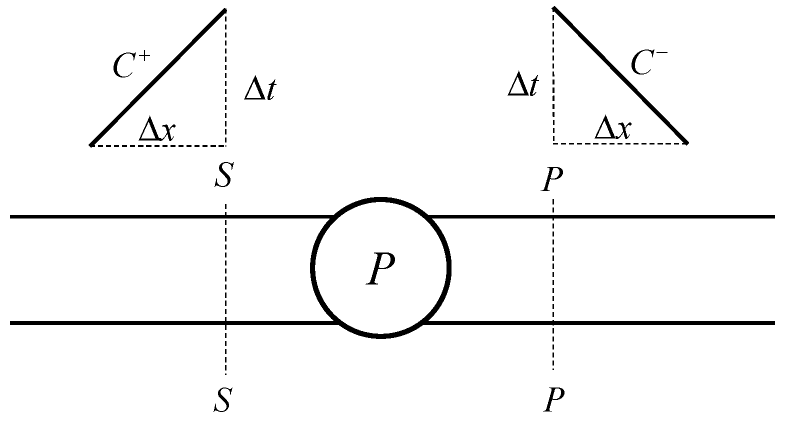
2.1. Calculation Theory of the Method of Characteristics for Transient Flow

The fundamental equations for establishing a transient flow calculation model in a pressurized, unsteady water pipeline include the motion differential equation and the continuity differential equation [27], as shown below:
g v 1 0 v a 2 g 0 1 × h x v x v t h t T = f v v 2 D v sin α ,
where h is the piezometric head, v is the flow velocity, t represents time, x represents the position coordinate, D represents the pipe diameter, g represents the acceleration due to gravity, f represents the friction factor along the pipe, a represents the wave speed of the water hammer, and α represents the angle of inclination of the pipe.
Solving through the method of characteristics and letting B = a / ( g A ) , R = f Δ x / ( 2 g D A 2 ) , the following equations can be derived
h P = C P + C M 2
q P = C P C M 2
where hP and qP are the pressure and flow rate at the computational node P. CP and CM are the coefficients corresponding to the aforementioned positive and negative characteristic lines:
C p C M = h A q A q A q A h B q b q B q B 1 B R
where hA and qA are the pressure and flow rate at the previous moment in the previous section. hB and qB are the pressure and flow rate at the previous moment of the next cross section.
Figure 1 shows a single pump connected to a pipeline. In the calculation of unsteady flow, the head balance equation of the pump at any time can be written as follows:
H S + t d h + H f V = H P
where HS is the pump inlet head, Hfv is the valve head loss, HP is the pump outlet head, and tdh represents the dynamic head of the pump.
The valve’s overflow characteristics and operation mode significantly impact the hydraulic transient process of the entire pipeline. To simulate the valve’s overflow characteristics of the valve, the relationship between the valve flow coefficient and the opening is established based on the local resistance coefficient when the valve is fully open and the relative opening of the gate.
During the transition process, it is assumed that the valve opening changes linearly or in stages:
τ t = f ( t )
where τ t is the valve opening function.
The flow coefficient and damping coefficient of the valve can be described by the following equations:
C d = f ( τ t )
ζ = 1 C d 2
where Cd is the flow coefficient of the valve and ζ is the damping coefficient of the valve.
Equation (7) can be determined through the valve characteristic curve. The discharge characteristics of the control valve are shown in Figure 2.
The boundary equation at the valve is defined as:
Q u p = Q d o w n
H u p = H d o w n + ζ V q u p 2 2 g A V 2
C + : h u p = C P B u q u p
C : h d o w n = C M + B d q d o w n
where Qup and hup are the flow and pressure upstream of the valve, Qdown and hdown are the flow and pressure downstream of the valve, and Bu and Bd are parameters of the forward characteristic equation and backward characteristic equation.
By combining the above equations, the valve’s upstream and downstream pressures and flow rates can be solved at any time.

2.2. Multi-Objective Optimization Method for Water Hammer Protection

2.2.1. Constructing the Sample Set Based on LHS-MCS

Latin Hypercube Sampling (LHS) ensures that the samples include all information about the changes in design variables. Consequently, for any parameter dimension, the projection of sample points in this dimension will be evenly distributed across the entire parameter range [28]. However, while LHS can cover the entire high-dimensional vector space, it may miss essential sample points in local areas when the space is highly non-uniform. By combining Monte Carlo Sampling (MCS), small random perturbations can be introduced to increase the randomness of sampling while maintaining uniform coverage, better-balancing uniformity, and randomness.

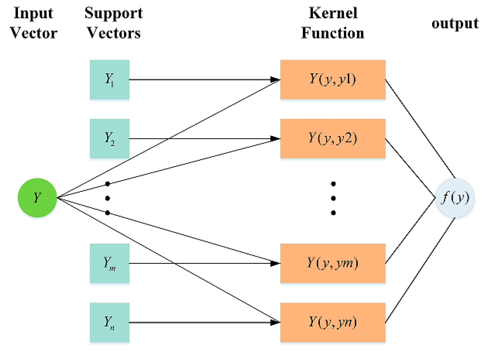
2.2.2. Support Vector Regression (SVR)

Support Vector Regression (SVR) algorithms handle high-dimensional space and small sample datasets excellently due to their kernel tricks, regularization, and epsilon-insensitive loss functions [29,30]. The structure of SVR is shown in Figure 3.
The valve closure parameters (first-stage pump station: fast-closure time t1, fast-closure angle θ1, slow-closure time t2, slow-closure angle θ2; second-stage pump station: fast-closure time t3, fast-closure angle θ3, slow-closure time t4, slow-closure angle θ4) are selected as optimization variables. A predictive model is constructed based on the SVR algorithm and simultaneously used as the objective function for the multi-objective optimization problem of water hammer protection in multi-stage pressurized water supply systems. The expressions are:
f H max = S V R ( t 1 , t 2 , θ 1 , θ 2 , t 3 , t 4 , θ 3 , θ 4 )
f V 1 , max = S V R ( t 1 , t 2 , θ 1 , θ 2 , t 3 , t 4 , θ 3 , θ 4 )
f V 2 , max = S V R ( t 1 , t 2 , θ 1 , θ 2 , t 3 , t 4 , θ 3 , θ 4 )

2.2.3. Combined Weighting Method

The most important aspect of converting a multi-objective optimization problem into a single-objective problem is determining the weight of each sub-objective. Different weights cause the algorithm to search for different optimal solutions, which may lead to an unreasonable engineering design. Combining the Analytic Hierarchy Process (AHP) with the Entropy Weight Method integrates subjective expert experience with objective data analysis.
By assigning weights through subjective judgment, suppose there are n sub-objectives. The elements aij of the judgment matrix A represent the importance of element i relative to element j. By solving Equation (16), the eigenvector w corresponding to the largest eigenvalue λmax of the judgment matrix A is obtained. This eigenvector is normalized to determine the weights of each sub-objective [31].
A w = λ max w
The Entropy Weight Method determines the weight of each index based on the measurement of uncertainty in the data. According to m evaluation objects and n valuation indices, matrix P is obtained [32]. To obtain the entropy weight of each evaluation index, dimensionless processing is performed on each index Zij using Equation (17).
Z i j = max ( p j ) p i j max ( p j ) min ( p j )
Proportion of each element pij
p i j = z i j i = 1 n z i j
Calculate the information entropy of each evaluation index ej
e j = 1 ln n i = 1 n p i j ln ( p i j ) , j = 1 , 2 , , m
Entropy weights wj are then expressed as
w j = 1 e j j = 1 m ( 1 e j )
Considering the strengths and weaknesses of the Analytical Hierarchy Process and the Entropy Weighting Method, a linear combination of subjective and objective weights is applied to determine the final weights.
w = α w 1 + β w 2

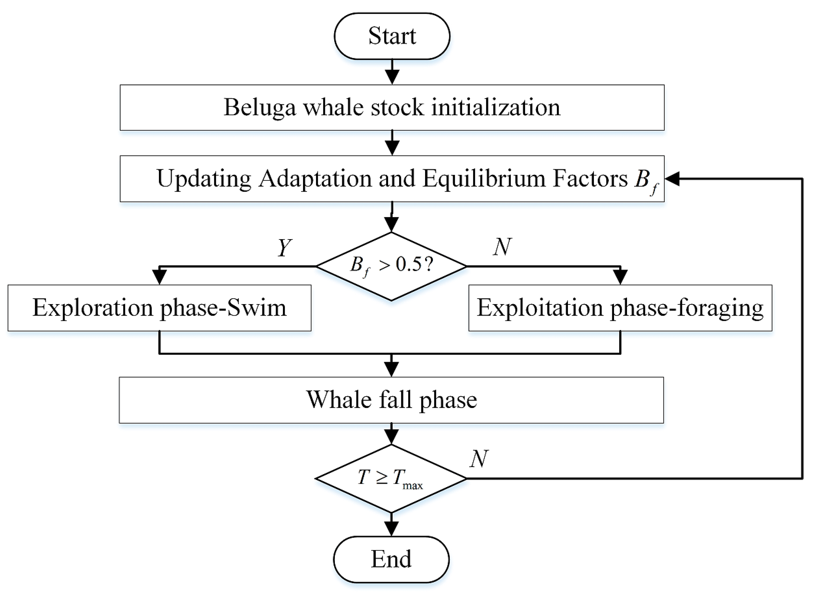
2.2.4. Beluga Whale Optimization (BWO)

The Beluga Whale Optimization (BWO) algorithm, proposed by Zhong et al. [33], is inspired by beluga whales’ swimming, foraging, and falling behaviors. During the exploration phase, BWO ensures the global search capability of the design space by randomly selecting beluga whales. In contrast, in the exploitation phase, it controls local searches within the design space. Additionally, the probability of whale falls is considered to simulate minor group variations. The flowchart of the algorithm is shown in Figure 4.

2.3. Multi-Objective Optimization Function

The magnitude of the pipeline pressure extremes and the dimensionless reverse speed of the pumps are critical to the safe operation of the water supply system. The optimization objectives are to minimize the maximum water hammer pressure of the water supply system and the maximum dimensionless reverse speed of the pumps in the first- and second-stage pump stations. The multi-objective optimization function can be expressed as a linear weighted sum of multiple sub-objective functions, namely:
F ( x ) = N 1 f H max + N 2 f v 1 , max + N 3 f v 2 , max
where N1, N2 and N3 are weighting factors representing the weight of each of the three sub-objective functions in the multi-objective function.
In multi-objective optimization, constraints define a transparent and bounded solution space by limiting the range of decision variables and influence the selection of the optimal solution. In the water hammer protection problem of multi-stage pressurized pump stations, the constraints include the reverse speed and reverse time constraints of the pumps, maximum water hammer pressure rise constraints, valve closure time constraints, and upper and lower limits of decision variables.
(1) Constraints on the centrifugal pump’s reverse speed and time. The maximum reverse speed of the centrifugal pump should not exceed 1.2 times the rated speed, and the duration of exceeding the rated speed should not exceed 2 min.
V max N R t r < 120 s
where Vmax is the maximum reverse speed of the pump, NR is the rated speed of the pump, and tr is the duration of exceeding the rated speed.
(2) Maximum water hammer pressure constraint. The maximum pressure should not exceed 1.3 to 1.5 times the rated outlet pressure of the pump.
H max < ( 1.3 ~ 1.5 ) H R
H ( i ) max < H ( i ) R
where H(i)max is the maximum water hammer pressure at each node, H(i)R is the allowable maximum pressure of the pipeline at each node, and HR is the rated outlet pressure of the pump.
(3) Constraints on valve closing time and angle. The fast-closing speed in the first stage is greater than the slow-closing speed in the second stage, and the valve is fully closed, i.e.,
θ 1 / t 1 > θ 2 / t 2 θ 3 / t 3 > θ 4 / t 4 θ 1 + θ 2 = 100 % θ 3 + θ 4 = 100 %
(4) Upper and lower limit constraints of decision variables. Based on the design experience of long-distance water supply systems in actual operation, the range of design variables is appropriately expanded and each decision variable must be within the specified range.
t 1 , min < t 1 < t 1 , max t 2 , min < t 2 < t 2 , max t 3 , min < t 3 < t 3 , max t 4 , min < t 4 < t 4 , max

2.4. Multi-Objective Optimization Model

Based on the transient flow calculation theory and the multi-objective optimization method for water hammer protection, the overall model was constructed after determining the multi-objective optimization function. The main steps are as follows:
(1) Determine the multi-objective water hammer protection optimization problem. Define input parameters and constraints according to the actual needs and technical specifications.
(2) Construct the sample set. Establish a transient flow calculation model based on the method of characteristics, construct the distribution of input parameters using the LHS-MCS hybrid sampling method, and simulate with the model to obtain the sample set.
(3) Build the SVR prediction model. Use K-fold cross-validation to define training and testing sets to train the regression prediction model.
(4) Use the SVR regression prediction model as the objective function in the BWO algorithm. Find the optimal solution based on the weight values determined by the analytic hierarchy process and entropy weight method.
(5) Simulate the optimal solution. Substitute the theoretically optimal solution found above into the transient flow calculation model to confirm the optimization effect.

3. Results and Discussion

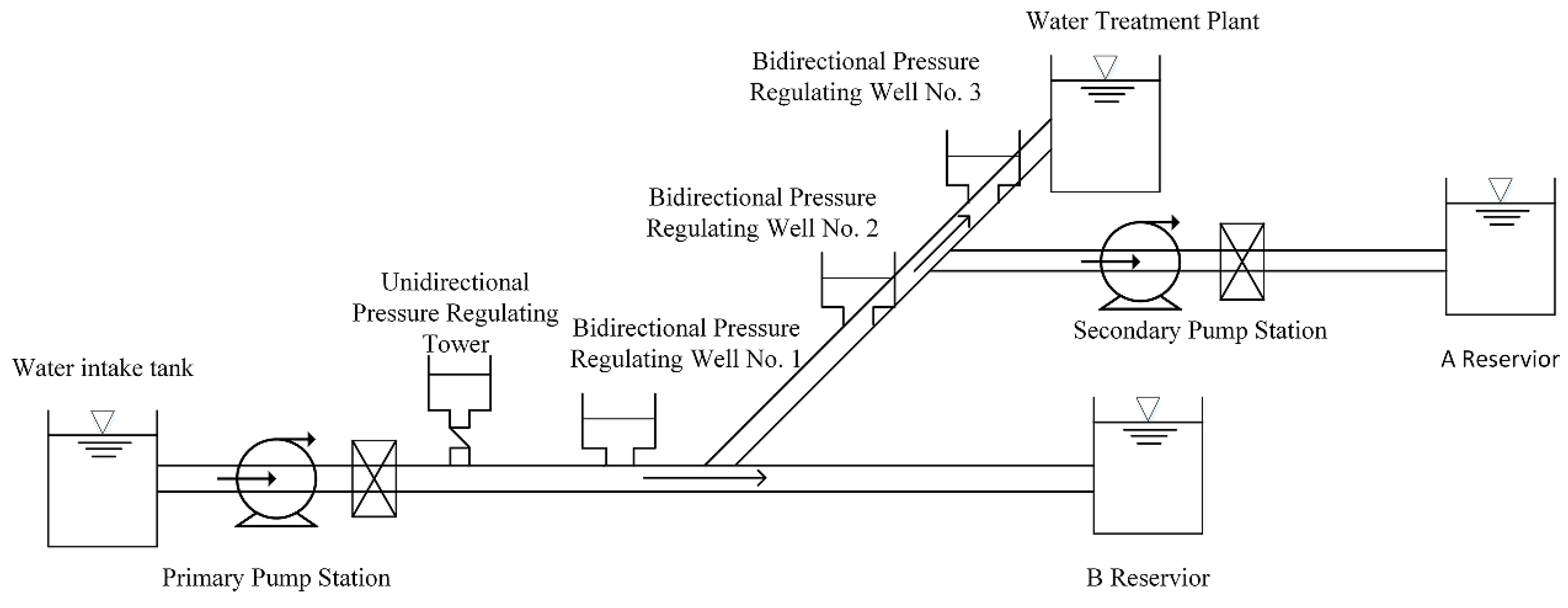
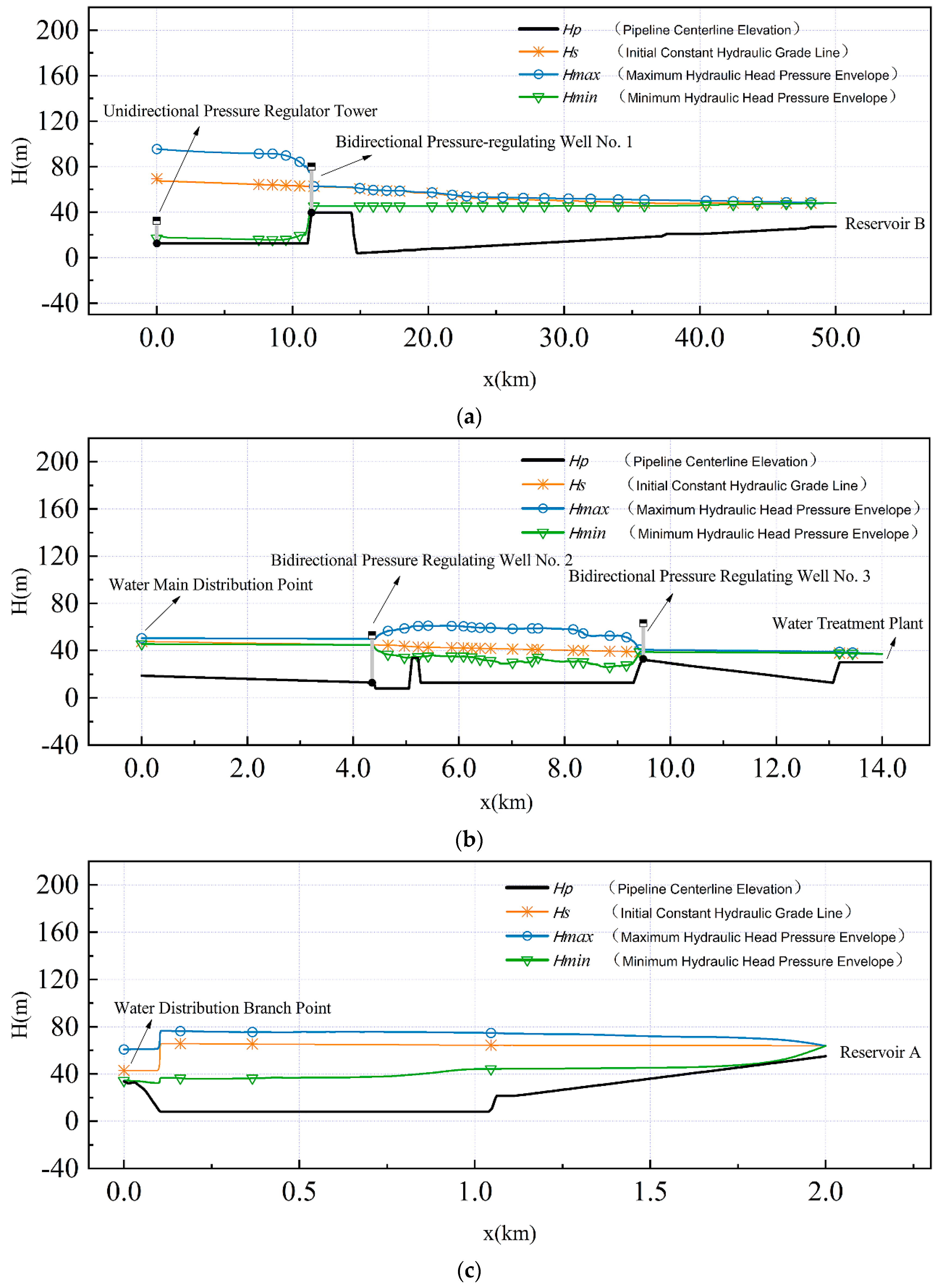
3.1. Project Introduction

Figure 5 is a simplified model diagram of the pipeline for a long-distance, multi-branch, multi-stage pressurized pump station water delivery system. The water conveyance project consists of a primary pump station, a secondary pump station, water conveyance tunnels, pipelines, an outlet reservoir, and a water plant. The entire water conveyance pipeline is divided into three sections: the main line from the primary pump station to Reservoir B is approximately 50 km long; the branch line from the main line junction to the water plant is approximately 14 km long; and the secondary branch line from the branch line junction to Reservoir A is approximately 2 km long. The inlet water level is 6 m, the water level of Reservoir A is 64 m, the water level of Reservoir B is 48 m, and the water level of the water plant is 37 m. This water conveyance line is characterized by a long overall distance, a large head, multiple branches, and high flow rates. To avoid large-scale negative pressure during the hydraulic transition, single-direction surge tanks and bi-directional surge wells are installed near the outlet of the primary pump station and at pipeline high points. The cross-sectional area of the single-direction surge tank is 79 m2, with a height of 10 m; the cross-sectional area of Surge Well No. 1 is 314.15 m2, with a height of 40 m; the cross-sectional area of Surge Well No. 2 is 75 m2, with a height of 40 m; and the cross-sectional area of Surge Well No. 3 is 75 m2, with a height of 20 m.

3.2. Comparison of Prediction Regression Models

3.2.1. Dataset Construction

Based on the LHS-MCS method to quickly establish the input distribution, selecting an appropriate sample size in machine learning is crucial. To balance the accuracy of the multi-objective optimization model and computational efficiency, a sample size of about ten times the number of input parameters is sufficient to train a well-performing model. Considering the number of valve closure parameters and computational efficiency in the multi-stage pressurized pump station water delivery system, the sample size is set to 100, i.e., 100 sets of t 1 , t 2 , θ 1 , θ 2 , t 3 , t 4 , θ 3 , θ 4 parameter groups. These parameter groups, obtained through hybrid sampling, are input into the hydraulic transient model for simulation, producing the maximum transient flow pressure values and the maximum dimensionless reverse speed for each pump station, thereby completing the dataset construction. Specific data are shown in Table 1.

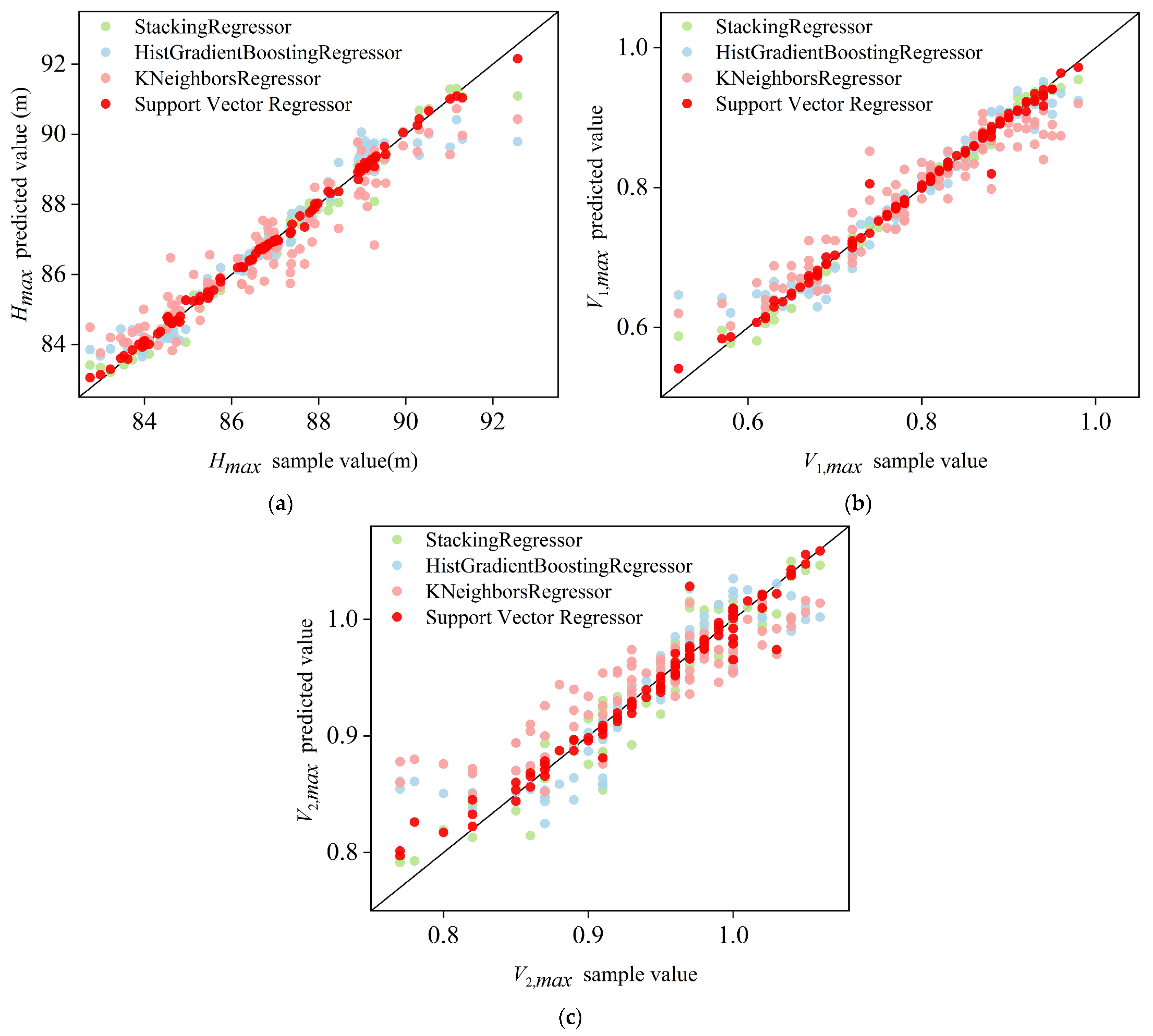
3.2.2. Comparison of Regression Algorithms

Root Mean Square Error (RMSE) and the coefficient of determination (R2) are the most commonly used metrics to evaluate the accuracy of algorithm performance. These two metrics are used to measure the performance of different regression algorithms. The formulas for RMSE and R2 are as follows:
R M S E = 1 m i = 1 m ( y i y ^ i ) 2
R 2 = 1 i = 1 m ( y i y ^ i ) 2 i = 1 m ( y i y ¯ i ) 2
where m is the number of samples, yi is the sample value, y ^ i is the predicted value of the regression model, and y ¯ i is the mean of all sample values.
To effectively assess the quality of the model, k-fold cross-validation is used to involve all the sample data in training and prediction. In this study, k is set to 10, with 90% of the sample set used as the training set and 10% as the test set, repeated ten times to obtain the final evaluation results.
Different regression algorithms have varying generalization abilities for the same dataset. Accurate prediction of the maximum water hammer pressure and the maximum reverse speed of pumping stations in a water delivery system is crucial for a multi-objective optimization problem. We use RMSE and R2 as the primary evaluation metrics. These two metrics allow us to quantitatively assess the accuracy and reliability of each regression algorithm’s predictions on each sub-objective function. The specific calculation results are shown in Table 2.
Table 2 shows the RMSE and R2 results for different regression prediction models. It can be seen that most regression models cannot accurately predict all three output targets simultaneously. However, the SVR model performs exceptionally well. For predicting the maximum water hammer pressure Hmax, the RMSE is 0.12 and R2 is 0.99; for predicting the primary pump station’s maximum dimensionless reverse speed V1,max, the RMSE is 0.01 and R2 is 0.99; and for predicting the secondary pump station’s maximum dimensionless reverse speed V2,max, the RMSE is 0.01 and R2 is 0.97.
As shown in Figure 6, the SVR model predicts multiple targets more accurately than StackingRegressor, HistGradientBoostingRegressor, and KNeighborsRegressor, with predicted values closer to the sample values. It can accurately construct the mathematical mapping relationship between the characteristic parameters of the two-stage valve closure and the target variables of the maximum water hammer pressure and the maximum dimensionless reverse speed of each pump station in the multi-stage pressurized pump station water delivery system.

3.3. Comparison of Optimization Algorithms

3.3.1. Weights Based on Different Biases

Three different decision biases can be identified in the decision analysis of long-distance water delivery systems. If the system prioritizes pipeline safety, the maximum water hammer pressure should be considered first, with the maximum dimensionless reverse speed of each pump station as a secondary indicator. If the system focuses more on the operational safety of pumps at each pump station, then the safety of the primary and secondary pump stations is considered more important. If there is no apparent bias, a balance between the maximum water hammer pressure and the maximum dimensionless reverse speed of the pump stations should be achieved. The weights based on the Analytic Hierarchy Process (AHP) and Entropy Weight Method are calculated to quantify these three decision biases, as shown in Table 3.

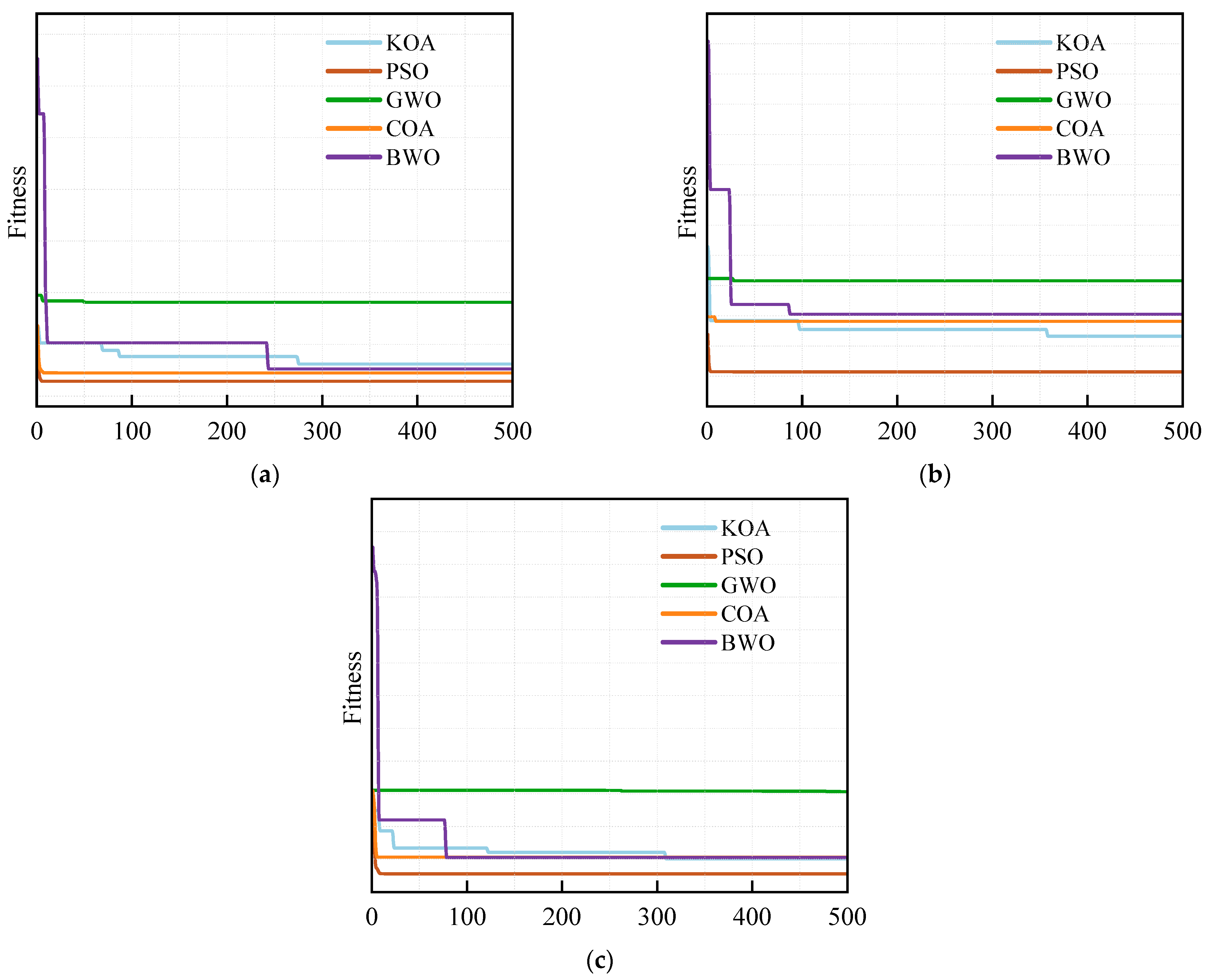
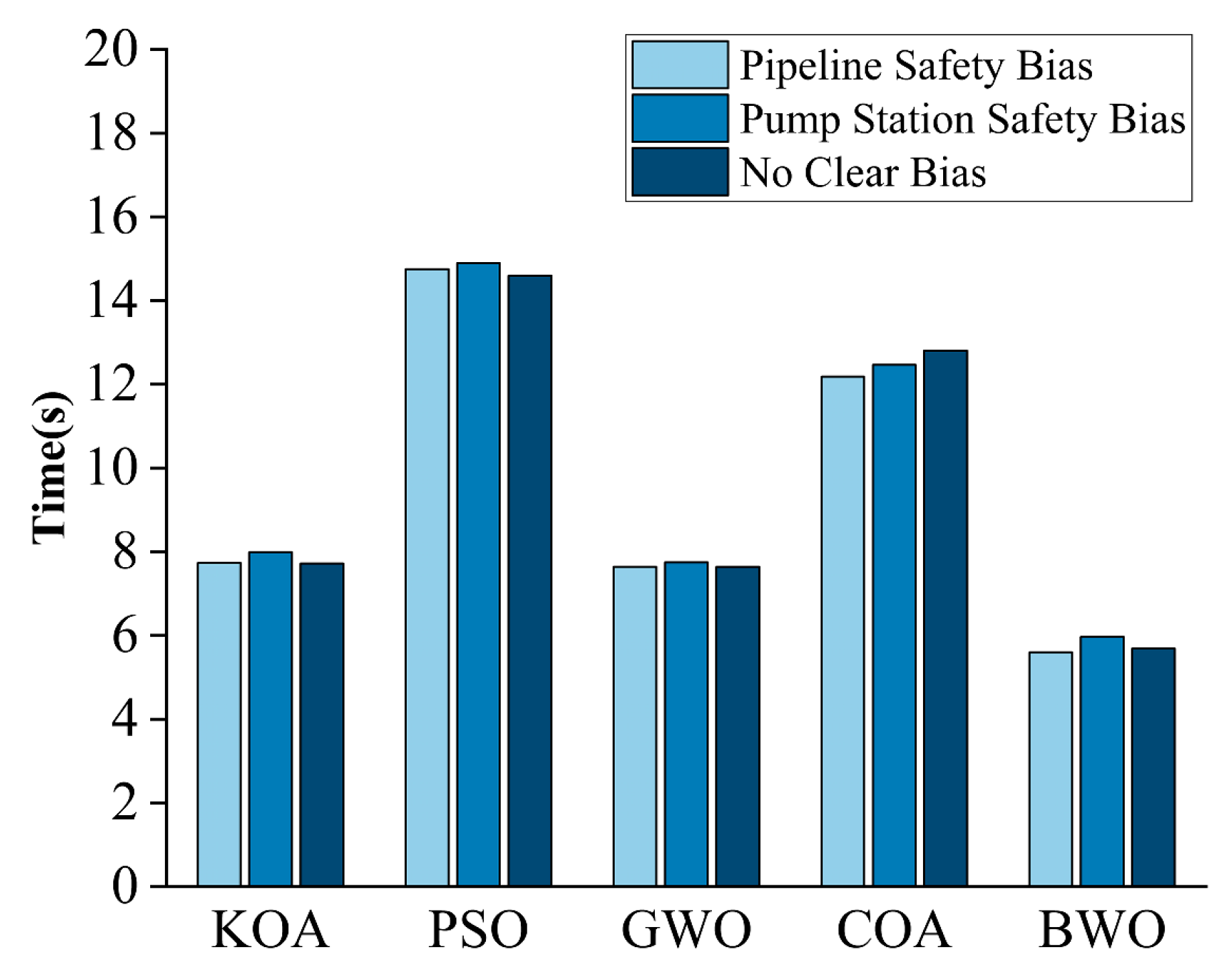
3.3.2. Effects of Different Optimization Algorithms

For specific problems, the effectiveness of optimization algorithms varies significantly. By comparing the BWO algorithm with classical optimization algorithms such as Particle Swarm Optimization (PSO) [34,35] and some emerging popular algorithms including the Kepler Optimization Algorithm (KOA) [36], Grey Wolf Optimization (GWO) [37], and Coati Optimization Algorithm (COA) [38], these algorithms were deeply analyzed and evaluated for optimal protection schemes under different biases.
The optimization results of the valve closure parameters for each pump station are shown in Table 4, detailing the optimal protection scheme parameters found by each algorithm under different test scenarios. t1 and θ1 are the fast-closing time and angle of the first stage for the primary pump station, t2 and θ2 are the slow-closing time and angle of the first stage for the primary pump station, t3 and θ3 are the fast-closing time and angle of the first stage for the secondary pump station, and t4 and θ4 are the slow-closing time and angle of the first stage for the secondary pump station.
The optimal schemes found by each optimization algorithm were substituted into the hydraulic transient model to calculate the maximum water hammer pressure during the hydraulic transition process, the maximum dimensionless reverse speed of the primary pump station, and the maximum dimensionless reverse speed of the secondary pump station. The multi-objective optimization function was calculated based on the combination of different biases, with the results shown in Table 5.
From Table 5, it can be seen that the maximum water hammer pressure and the maximum dimensionless reverse speed of the pump stations cannot be optimized simultaneously. A reduction in the maximum water hammer pressure inevitably accompanies an increase in the reverse speed and vice versa. Using F(x) as the comprehensive protection effectiveness evaluation index, the comprehensive protection effectiveness ranking of the five optimization algorithms under the pipeline safety bias is BWO > PSO > KOA > GWO > COA, under the pump station safety bias is BWO > PSO > KOA > COA > GWO, and under no clear bias is BWO > PSO > KOA > COA > GWO. BWO’s F(x) values under the three conditions are 34.11, 14.46, and 23.28, respectively, which are all better than the other four optimization algorithms, showing potential for further exploration and application in similar engineering problems.
Figure 7 presents a comparative analysis of the number of iterations of the five optimization algorithms. Through in-depth research, it can be observed that KOA has a significantly slower convergence speed. Although PSO and COA can complete the optimization process in fewer iterations, they struggle to achieve a global search and tend to fall into local optima. GWO’s optimization performance is not ideal, as it has limited overall optimization capability.
In contrast, the BWO algorithm balances the number of iterations and global search capability. BWO maintains an efficient global search capability within an acceptable number of iterations, demonstrating strong optimization performance. This performance indicates that the BWO algorithm has excellent exploration and exploitation capabilities, effectively avoiding local optima and exploring a broader solution space.
Computational time is a key indicator for evaluating the efficiency of optimization algorithms. Figure 8 shows the computation time required for each algorithm to complete iterations under different biases. Under the pipeline safety bias, the computation times for KOA, PSO, GWO, COA, and BWO are 7.74 s, 14.75 s, 7.63 s, 12.18 s, and 5.6 s, respectively. Under the pump station safety bias, the corresponding computation times are 7.99 s, 14.89 s, 7.75 s, 12.47 s, and 5.97 s. Under no clear bias, the computation times are 7.72 s, 14.6 s, 7.74 s, 12.81 s, and 5.69 s, respectively.
Further analysis shows that the average computation time for the KOA algorithm is 7.82 s, for the PSO algorithm it is 14.75 s, for the GWO algorithm it is 7.68 s, for the COA algorithm it is 12.81 s, and for the BWO algorithm it is 5.75 s. Comparing these data, it is found that the BWO algorithm has the shortest average optimization time among all considered algorithms, with efficiency improvements of 26.47%, 61.02%, 25.13%, and 55.11% over the KOA, PSO, GWO, and COA algorithms, respectively. This result indicates that the BWO algorithm exhibits excellent optimization efficiency on the objective function constructed based on the SVR regression model.
After comparing key performance indicators such as comprehensive protection effectiveness, convergence performance, and computation time, the results show that the BWO algorithm performs significantly better than others.

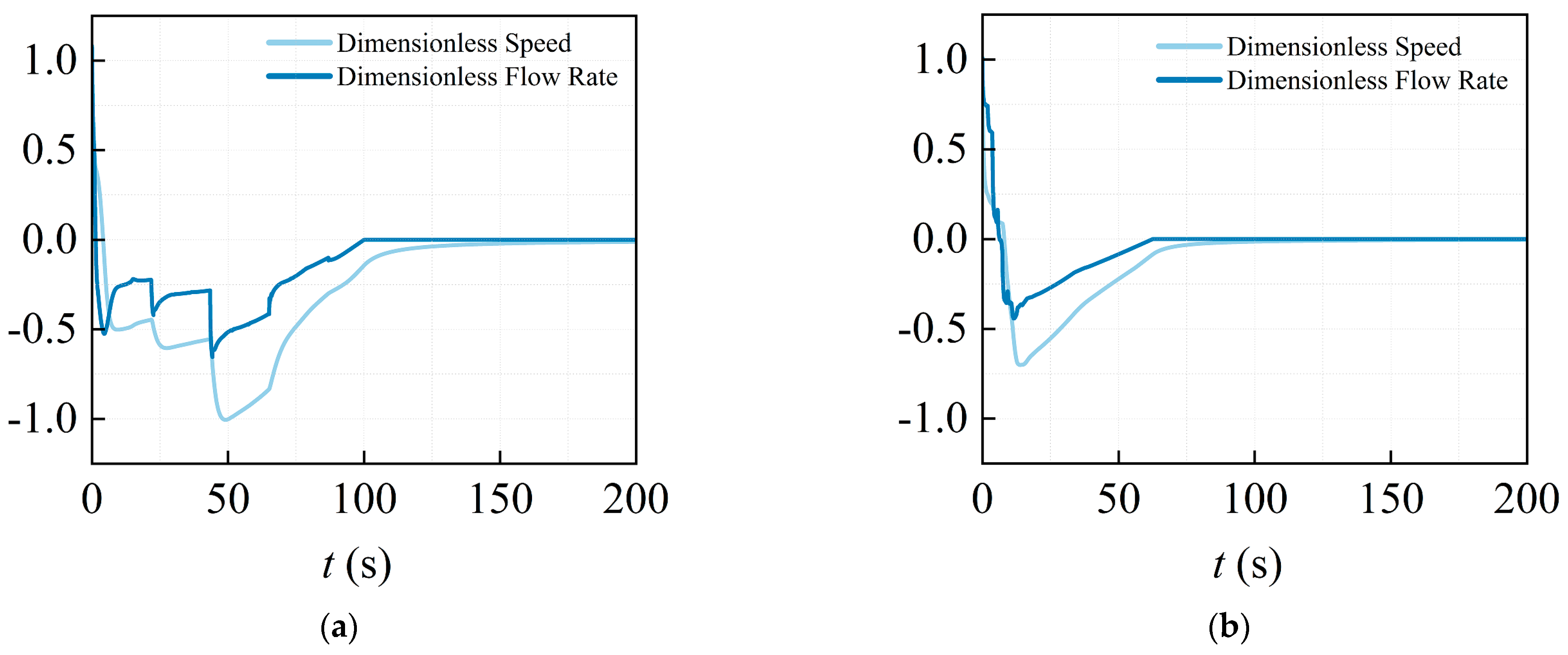
3.4. Verification of Theoretical Solution

For the long-distance, multi-branch, multi-stage pressurized pump station water delivery system, different optimal solutions can meet the design requirements. Due to the engineering requirements that simultaneously consider the safety of the pipeline and pump stations, the unbiased optimization scheme is selected for verification.
In simultaneous accidents at all pump stations, the valves after the pumps at the first-stage pump station adopt a two-stage closure: 80% fast closure in 15 s in the first stage and 20% slow closure in 85 s in the second stage. For the second-stage pump station, the valves adopt a 90% fast closure in 5 s in the first stage and 10% slow closure in 57.5 s in the second stage. The hydraulic transition process of the water supply line was analyzed using a hydraulic transient model for a long-distance multi-stage pressurized pump station water supply system. The pressure distribution along the entire line is shown in Figure 9. It can be seen that the pressure head along the entire line meets the safety requirements of the water supply system design. The maximum water hammer pressure of the water supply system is 84.2 m.
As shown in Figure 10, the primary pump station starts to reverse 4.13 s after the accident shutdown, reaching the maximum dimensionless reverse speed of 1 after 49.04 s. The secondary pump station starts to reverse 8.04 s after the accident shutdown, reaching the maximum dimensionless reverse speed of 0.701 after 13.71 s. The reverse speeds of each pump station do not exceed 1.2 times the rated speed and the reverse flow duration is less than 120 s, meeting the pump station design standards.

4. Conclusions

For the optimization problem of water hammer protection in long-distance, multi-stage pressurized pump station water delivery systems, a multi-objective optimization coupling model with decision-maker preferences was constructed based on the SVR and BWO optimization algorithms. This model employs the SVR algorithm to establish the mathematical mapping between the valve closure parameters of multi-stage pump stations, the maximum water hammer pressure, and the maximum dimensionless reverse speed of each pump station. The objective functions are minimizing the maximum water hammer pressure and the maximum dimensionless reverse speed. The BWO optimization algorithm searches for the optimal water hammer protection scheme under different biases. Based on the above results and discussion, the following conclusions can be drawn:
(1) The Support Vector Regression algorithm exhibits superior prediction accuracy and generalization ability for each sub-objective. The RMSE and R2 between the actual and predicted values of the maximum water hammer pressure are 0.12 and 0.99, respectively; the RMSE and R2 between the actual and predicted values of the primary pump station’s maximum dimensionless reverse speed are 0.01 and 0.99, respectively; and the RMSE and R2 between the actual and predicted values of the secondary pump station’s maximum dimensionless reverse speed are 0.01 and 0.97, respectively.
(2) The BWO optimization algorithm significantly outperforms PSO, GWO, KOA, and COA in terms of convergence performance and computation time. The valve closure schemes identified by BWO provide the best comprehensive protection effects. The SVR-BWO coupling model can find optimal schemes under different biases in a short time, allowing decision-makers to select the appropriate scheme based on the actual needs, thereby reducing manual calculation costs and improving efficiency. This case study demonstrates that the model can effectively fit highly nonlinear correlated datasets with small samples and quickly identify the optimal water hammer protection scheme for long-distance, multi-stage pressurized pump stations water delivery systems. It effectively resolves multi-objective optimization problems with multiple nonlinear correlated input parameters and provides solutions for other multi-objective optimization engineering problems influenced by multiple factors.

Author Contributions

Conceptualization, writing—original draft preparation, Y.D.; writing—review and editing, W.W. and G.S. All authors have read and agreed to the published version of the manuscript.

Funding

This study was supported by the National Natural Science Foundation of China (Grant Nos. 52079122, 52379080).

Data Availability Statement

The original contributions presented in the study are included in the article, further inquiries can be directed to the corresponding author.

Conflicts of Interest

The authors declare no conflicts of interest.

References

  1. Panov, L.V.; Chirkov, D.V.; Cherny, S.G.; Pylev, I.M. Numerical simulation of pulsation processes in hydraulic turbine based on 3d model of cavitating flow. Thermophys. Aeromech. 2014, 21, 31–43. [Google Scholar] [CrossRef]
  2. Leishear, R.A. Water hammer causes water main breaks. J. Press. Vessel Technol. 2020, 142, 021402. [Google Scholar] [CrossRef]
  3. Chen, T.; Ren, Z.; Xu, C.; Loxton, R. Optimal boundary control for water hammer suppression in fluid transmission pipelines. Comput. Math. Appl. 2015, 69, 275–290. [Google Scholar] [CrossRef]
  4. Bergant, A.; Simpson, A.; Sijamhodzic, E. Water hammer analysis of pumping systems for control of water in underground mines. In Proceedings of the Mine Water Congress, Ljubljana, Slovenia, 25–30 September 1991; pp. 9–20. [Google Scholar]
  5. Sciamarella, D.; Artana, G. A water hammer analysis of pressure and flow in the voice production system. Speech Commun. 2009, 51, 344–351. [Google Scholar] [CrossRef]
  6. Asli, K.H.; Naghiyev, F.B.O.; Haghi, A.K. Some aspects of physical and numerical modeling of water hammer in pipelines. Nonlinear Dyn. 2010, 60, 677–701. [Google Scholar] [CrossRef]
  7. Erath, W.; Nowotny, B.; Maetz, J. Modelling the fluid structure interaction produced by a waterhammer during shutdown of high-pressure pumps. Nucl. Eng. Des. 1999, 193, 283–296. [Google Scholar] [CrossRef]
  8. Fu, X.; Li, D.; Wang, H.; Qin, D.; Wei, X. Cavitation mechanism and effect on pump power-trip transient process of a pumped-storage unit. J. Energy Storage 2023, 66, 107405. [Google Scholar] [CrossRef]
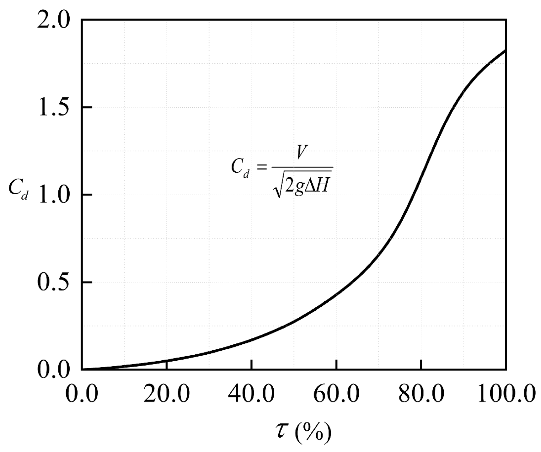
  9. Wan, W.; Lian, J.; Li, Y. Influence of valve system discharge coefficient on hydraulic transients. J. Tsinghua Univ. (Sci. Technol.) 2005, 45, 1198–1201. [Google Scholar]
  10. Romuald, B.; Jian, Z.; Dong, Y.X.; Claire, D. Assessment and performance evaluation of water hammer in hydroelectric plants with hydropneumatic tank and pressure regulating valve. J. Press. Vessel Technol. 2021, 143, 041401. [Google Scholar] [CrossRef]
  11. Liu, W.; Tan, P.; Yang, J. Study on two-stage closure of valve stroking for water hammer protection of unexpected pump-stop. Fluid Mach. 2020, 48, 53–57. [Google Scholar]
  12. Wan, W.Y.; Li, F.Q. Sensitivity analysis of operational time differences for a pump-valve system on a water hammer response. J. Press. Vessel Technol. 2016, 138, 011303. [Google Scholar] [CrossRef]
  13. Lu, M.; Liu, X.; Xu, G.; Tian, Y. Optimal pump-valve coupling operation strategy of complex long-distance water-conveyance systems based on moc. Ain Shams Eng. J. 2024, 15, 102318. [Google Scholar] [CrossRef]
  14. Han, Y.; Shi, W.D.; Xu, H.; Wang, J.B.; Zhou, L. Effects of closing times and laws on water hammer in a ball valve pipeline. Water 2022, 14, 1497. [Google Scholar] [CrossRef]
  15. Neyestanaki, M.K.; Dunca, G.; Jonsson, P.; Cervantes, M.J. A comparison of different methods for modelling water hammer valve closure with cfd. Water 2023, 15, 1510. [Google Scholar] [CrossRef]
  16. Zhao, S.G.; Wang, M.N.; Yi, W.H.; Yang, D.; Tong, J.J. Intelligent classification of surrounding rock of tunnel based on 10 machine learning algorithms. Appl. Sci. 2022, 12, 2656. [Google Scholar] [CrossRef]
  17. Dhakal, R.; Zhou, J.X.; Palikhe, S.; Bhattarai, K.P. Hydraulic optimization of double chamber surge tank using nsga-ii. Water 2020, 12, 455. [Google Scholar] [CrossRef]
  18. Hao, R.A.; Bai, Z.X. Comparative study for daily streamflow simulation with different machine learning methods. Water 2023, 15, 1179. [Google Scholar] [CrossRef]
  19. Lu, M.S.; Hou, Q.Y.; Qin, S.J.; Zhou, L.H.; Hua, D.; Wang, X.X.; Cheng, L. A stacking ensemble model of various machine learning models for daily runoff forecasting. Water 2023, 15, 1265. [Google Scholar] [CrossRef]
  20. Li, J.Y.; Yuan, X. Daily streamflow forecasts based on cascade long short-term memory (lstm) model over the yangtze river basin. Water 2023, 15, 1019. [Google Scholar] [CrossRef]
  21. Xu, C.; Hux, L.; Wang, R.; Wang, X.; Tian, J. Multi-objective optimzation study of flow field characteristics in forward intake structure of pumping station. Shuili Xuebao/J. Hydraul. Eng. 2024, 55, 167–178. [Google Scholar]
  22. Brunton, S.L.; Noack, B.R.; Koumoutsakos, P. Machine Learning for Fluid Mechanics. Annu. Rev. Fluid Mech. 2020, 52, 477–508. [Google Scholar] [CrossRef]
  23. Bazargan-Lari, M.R.; Kerachian, R.; Afshar, H.; Bashi-Azghadi, S.N. Developing an optimal valve closing rule curve for real-time pressure control in pipes. J. Mech. Sci. Technol. 2013, 27, 215–225. [Google Scholar] [CrossRef]
  24. Lai, X.; Li, C.; Zhou, J.; Zhang, N. Multi-objective optimization of the closure law of guide vanes for pumped storage units. Renew. Energy 2019, 139, 302–312. [Google Scholar] [CrossRef]
  25. Cao, Z.; Xia, Q.; Guo, X.J.; Lu, L.; Deng, J.Q. A novel surge damping method for hydraulic transients with operating pump using an optimized valve control strategy. Water 2022, 14, 1576. [Google Scholar] [CrossRef]
  26. Lei, L.; Chen, D.; Ma, C.; Chen, Y.; Wang, H.; Chen, H.; Zhao, Z.; Zhou, Y.; Mahmud, A.; Patelli, E. Optimization and decision making of guide vane closing law for pumped storage hydropower system to improve adaptability under complex conditions. J. Energy Storage 2023, 73, 109038. [Google Scholar] [CrossRef]
  27. Wylie, E.B.; Streeter, V.L. Fluid Transients; McGraw-Hill International Book Co.: New York, NY, USA, 1978. [Google Scholar]
  28. Shields, M.D.; Zhang, J.X. The generalization of latin hypercube sampling. Reliab. Eng. Syst. Saf. 2016, 148, 96–108. [Google Scholar] [CrossRef]
  29. Smola, A.J.; Schölkopf, B. A tutorial on support vector regression. Stat. Comput. 2004, 14, 199–222. [Google Scholar] [CrossRef]
  30. Yu, X.; Zhang, X.Q.; Qin, H. A data-driven model based on fourier transform and support vector regression for monthly reservoir inflow forecasting. J. Hydro-Environ. Res. 2018, 18, 12–24. [Google Scholar] [CrossRef]
  31. Saaty, R.W. The analytic hierarchy process—what it is and how it is used. Math. Model. 1987, 9, 161–176. [Google Scholar] [CrossRef]
  32. Zhu, Y.X.; Tian, D.Z.; Yan, F. Effectiveness of entropy weight method in decision-making. Math. Probl. Eng. 2020, 2020, 3564835. [Google Scholar] [CrossRef]
  33. Zhong, C.T.; Li, G.; Meng, Z. Beluga whale optimization: A novel nature-inspired metaheuristic algorithm. Knowl.-Based Syst. 2022, 251, 109215. [Google Scholar] [CrossRef]
  34. Kennedy, J.; Eberhart, R. Particle swarm optimization. In Proceedings of the ICNN’95—International Conference on Neural Networks, Perth, WA, Australia, 27 November 27–1 December 1995. [Google Scholar]
  35. Eberhart, R.; Kennedy, J. A new optimizer using particle swarm theory. In Proceedings of the Sixth International Symposium on Micro Machine and Human Science, MHS’95, Nagoya, Japan, 4–6 October 1995. [Google Scholar]
  36. Abdel-Basset, M.; Mohamed, R.; Azeem, S.A.A.; Jameel, M.; Abouhawwash, M. Kepler optimization algorithm: A new metaheuristic algorithm inspired by kepler’s laws of planetary motion. Knowl.-Based Syst. 2023, 268, 110454. [Google Scholar] [CrossRef]
  37. Mirjalili, S.; Mirjalili, S.M.; Lewis, A. Grey wolf optimizer. Adv. Eng. Softw. 2014, 69, 46–61. [Google Scholar] [CrossRef]
  38. Dehghani, M.; Montazeri, Z.; Trojovská, E.; Trojovský, P. Coati optimization algorithm: A new bio-inspired metaheuristic algorithm for solving optimization problems. Knowl.-Based Syst. 2023, 259, 110011. [Google Scholar] [CrossRef]
Figure 1. Characteristic lines of the boundary condition of a pump.
Water 16 01728 g001
Figure 2. Discharge characteristics of the control valve.
Water 16 01728 g002
Figure 3. The structure of SVR.
Water 16 01728 g003
Figure 4. Flowchart of Beluga Whale Optimization algorithm.
Water 16 01728 g004
Figure 5. Simplified diagram of the water delivery system model.
Water 16 01728 g005
Figure 6. Performance of regression model predictions. (a) Maximum water hammer pressure Hmax; (b) dimensionless reverse speed of primary pump station V1,max; and (c) dimensionless reverse speed of secondary pump station V2,max.
Water 16 01728 g006
Figure 7. Number of iterations of different algorithms. (a) Pipeline safety bias. (b) Pump station safety bias. (c) No clear bias.
Water 16 01728 g007
Figure 8. Computation time of different algorithms.
Water 16 01728 g008
Figure 9. The pressure distribution of the water delivery system: (a) Pressure envelope of main conveyance line. (b) Pressure envelope of branch line. (c) Pressure envelope of secondary branch line.
Water 16 01728 g009
Figure 10. Dimensionless speed and flow of each pump station. (a) Primary pump station. (b) Secondary pump station.
Water 16 01728 g010
Table 1. Sample set based on LHS-MCS method.
Serial Numbert1t2 θ 1 θ 2 t3t4 θ 3 θ 4 Hmax (m)V1,maxV2,max
19.7287.5889.7710.237.5158.9789.2210.7892.570.520.78
28.1085.3185.7314.277.3960.1586.113.988.270.730.92
36.0689.9386.4213.586.2860.0887.1312.8788.90.690.87
4686.5586.0613.949.557.7685.1514.8589.30.691
511.6887.9484.9715.037.7856.384.515.585.50.830.97
610.6686.1887.3112.697.3161.887.0312.9788.940.680.88
710.2189.2786.8513.159.1958.8984.5415.4687.910.721
810.3886.3583.316.78.4660.0887.7312.2784.670.880.87
912.0987.6281.9418.068.8358.1884.4215.5887.350.940.99
106.5787.6884.2415.767.8459.2484.815.286.750.80.96
1111.0688.5487.7812.228.2657.182.6117.3988.960.671.02
1210.3787.6282.117.98.5260.0788.811.283.460.930.82
139.9589.0789.210.86.8463.7385.0914.9191.30.570.95
147.887.6383.4116.597.9857.6486.2413.7685.450.850.92
157.5585.5186.0913.915.9257.9584.0115.9988.910.70.97
9110.9386.0685.6514.357.563.9885.7114.2986.830.780.93
9210.4488.5983.916.16.7259.3585.4814.5284.810.870.93
936.5586.8683.9516.058.8163.0285.5914.4186.640.80.96
9411.8186.581.9218.085.357.4585.7614.2482.990.940.91
957.2787.3382.9117.096.6862.8983.9616.0485.280.860.98
9612.586.2484.1715.836.6661.2982.8317.1784.730.871
977.4488.1481.518.55.6360.2286.8313.1783.870.920.87
989.5688.5883.2516.759.0763.8688.7111.2984.520.880.86
9914.3488.3684.9415.069.8859.6385.2714.7384.540.861
1007.9887.1282.4117.596.5560.0584.9315.0784.630.890.95
Table 2. Prediction accuracy of regression models.
Regression ModelHmaxV1,maxV2,max
RMSER2RMSER2RMSER2
Random Forest Regressor0.690.710.020.920.020.89
Support Vector Regressor0.120.990.010.990.010.97
GradientBoostingRegressor0.790.650.020.940.020.93
LinearRegression0.750.690.020.960.020.93
Ridge0.680.840.030.880.030.79
HistGradientBoostingRegressor0.530.920.020.940.020.8
AdaBoostRegressor0.370.950.030.880.020.81
ExtraTreesRegressor0.670.730.020.950.060.31
StackingRegressor0.270.980.020.980.020.88
RidgeCV1.370.330.030.90.020.94
Lasso1.30.390.060.570.060.22
KNeighborsRegressor0.740.830.040.830.030.68
PoissonRegressor0.620.760.020.910.020.91
GammaRegressor0.980.690.050.690.030.72
ElasticNet0.980.690.050.680.030.72
HuberRegressor0.970.690.050.690.030.72
Table 3. Weights of sub-objectives with different biases.
Design BiasHmaxV1,maxV2,max
Pipeline Safety Priority0.4030.340.257
Station Safety Priority0.1630.5090.328
No Clear Bias0.2690.4080.323
Table 4. Optimal protection schemes under different biases.
Protection Schemes under
Different Biases
Optimization
Algorithm
t1t2 θ 1 θ 2 t3t4 θ 3 θ 4
Optimal Scheme Under Pipeline Safety BiasKOA14.0986.3980207.6463.4283.8816.12
PSO14.589.6280208.0561.286.9613.04
GWO10.4188.0384.3315.677.0458.3785.514.5
COA13.485802055588.411.6
BWO14.8289.8180207.8561.3787.612.4
Optimal Scheme Under Pump Station Safety BiasKOA12.2386.8780207.7457.785.2614.74
PSO13.3286.3580.0219.986.5861.3489.8310.17
GWO8.8788.8489.310.77.8164.2282.5517.45
COA13.9387.7582.3917.61561.299010
BWO158580205559010
Optimal Scheme Under No Clear BiasKOA13.018580205.3358.6983.7716.23
PSO12.8289.8580.4719.537.561.2888.6711.33
GWO9.6886.2580.619.48.0762.9389.2710.73
COA11.6489.8281.6818.3256588.9611.04
BWO15858020557.59010
Table 5. Summary of optimal protection scheme effects found by different optimization algorithms under different biases.
Protection Schemes under
Different Biases
Optimization
Algorithm
Hmax (m)V1,maxV2,maxF(x)
Optimal Scheme Under Pipeline Safety BiasKOA84.2510.98734.54
PSO83.481.0140.89334.22
GWO85.320.8440.93234.91
COA85.251.0270.92534.94
BWO83.261.0290.7934.11
Optimal Scheme Under Pump Station Safety BiasKOA85.310.9890.94514.72
PSO84.790.9950.73514.57
GWO91.920.5451.02615.59
COA86.610.9480.70614.83
BWO84.210.69714.46
Optimal Scheme Under No Clear BiasKOA85.280.9890.96723.66
PSO84.230.9920.81123.32
GWO88.220.9490.78724.37
COA86.40.9540.77523.88
BWO84.210.70123.28
Disclaimer/Publisher’s Note: The statements, opinions and data contained in all publications are solely those of the individual author(s) and contributor(s) and not of MDPI and/or the editor(s). MDPI and/or the editor(s) disclaim responsibility for any injury to people or property resulting from any ideas, methods, instructions or products referred to in the content.

