Brief Report

Identifying a Minimum Time Period of Streamflow Recession Records to Analyze the Behavior of Groundwater Storage Systems: A Study in Heterogeneous Chilean Watersheds

1
Department of Environmental Engineering, Universidad de Concepción, Concepción 4070386, Chile
2
Centro de Ciencias Ambientales EULA-Chile, Universidad de Concepción, Concepción 4070386, Chile
3
Department of Civil Engineering, Universidad Católica de la Santísima, Concepción 4090541, Chile
4
Centro de Investigación en Biodiversidad y Ambientes Sustentables (CIBAS), Concepción 4090541, Chile
5
Department of Water Resources, Universidad de Concepción, Chillán 3812120, Chile
6
Centro de Recursos Hídricos para la Agricultura y Minería (CRHIAM), Centro ANID Fondap, Concepción 4070411, Chile
7
Ingeniería EMO-LLS Ltd.a., Concepción 409007, Chile
*
Author to whom correspondence should be addressed.
Water 2024, 16(12), 1741; https://doi.org/10.3390/w16121741
Submission received: 18 April 2024 / Revised: 4 June 2024 / Accepted: 11 June 2024 / Published: 20 June 2024
(This article belongs to the Topic Advances in Hydrogeological Research)

Abstract

:
Aquifers are complex systems that present significant challenges in terms of characterization due to the lack or absence of watershed-scale hydrogeological information. An alternative to address the need to characterize watershed-scale aquifer behavior is recession flow analysis. Recession flows are flows sustained by groundwater release from the aquifer. Aquifer behavior can be characterized using recession flow records available from gauging stations, and therefore an indirect measure of aquifer behavior is obtained through watershed-scale recession flow records and analysis. This study seeks to identify the minimum time period necessary to characterize the behavior of groundwater storage systems in watersheds with different geological, morphological, and hydrological characteristics. To this end, various watersheds in south-central Chile underwent recession flow analysis, with eight time periods considered (2, 3, 4, 5, 10, 15, 20, and 25 years). The results indicate that 25 years of records are sufficient for the characterization of watershed-scale aquifer behavior, along with the representation of the groundwater storage-release (S-Q) process in watersheds with different geological, morphological, and hydrological characteristics. Additionally, the results show that an initial characterization of the groundwater system behavior in watersheds with different geological characteristics can be carried out with two years of records. This information could be important for practical engineering and the study of groundwater systems in watersheds with limited hydrological and hydrogeological information.

1. Introduction

Characterization of groundwater systems is often a complex task because watershed-scale hydrogeological information is limited due to data scarcity, limitations of monitoring techniques, or access difficulties due to geological and/or topographic factors [1,2].
Meanwhile, to characterize the temporality of hydrological processes or the hydrogeological functioning of watersheds, complete hydrological or hydrogeological data series are required (e.g., spatially distributed groundwater levels in a watershed). However, hydrogeological time series spatially distributed for these studies are generally limited or nonexistent, and when they are available, they tend to present discontinuities [3].
The characterization of groundwater systems is generally performed using in situ measurements and techniques such as geologic mapping [4], groundwater level measurement [5,6,7], hydrogeochemistry [8,9,10,11], geophysics [3,12,13], baseflow separation [14,15], recession flow analysis [16,17,18,19], and conceptual and numerical modeling [20,21], among others. Most of these techniques can be logistically complicated to carry out and economically costly [22]. In addition, because groundwater is located underground, techniques to characterize it are indirect measurements that entail a degree of uncertainty, along with a high cost of acquiring the information [23].
An alternative for indirectly providing hydrogeological information is the recording of river flows that are fed by groundwater, known as “recession flows”. These flows reflect the delayed release of groundwater into rivers, allowing flows to be maintained during periods of limited precipitation [24]. Recession flow analysis has been widely used to study groundwater systems. Via the power-law relationship and parameters a and b presented in Equation (1) proposed by Brutsaert and Nieber [25], it is possible to indirectly ascertain the watershed-scale hydrogeological behavior of a groundwater storage and release system. Parameter b represents the recession behavior, while parameter a represents the aquifer properties of the watersheds.
Recession flow analysis is a simple and valuable tool for characterizing the dynamics of the behavior of the groundwater storage and release process of an aquifer [26,27,28,29], as it provides information on watershed functioning, related to runoff generation, storage retention, and baseflow dynamics [30]. For example, Tashie et al. [31] analyzed the recession behavior of 1027 streams in the United States. The authors found that heterogeneous watershed characteristics (e.g., topography, permeability, etc.) lead to different groundwater storage-release behaviors. Similarly, Li and Ameli [32] found that the streamflow recession behavior strongly depends on different geological, morphological, and hydrological watershed characteristics. Parra et al. [28] recently analyzed recession behavior in several Chilean watersheds through moving-time-window analysis and how this behavior was related to geomorphological and climatic variability characteristics. The authors found that the recession behavior in wet periods tends toward fast drainage, while in dry periods it tends toward slow drainage.
The recession flow analysis presents advantages relative to other methodologies. Among these advantages is greater spatial availability of records as well as greater temporal resolution of the data needed for analysis (only flow records are required). This methodology has a low cost because it uses the existing surface water monitoring network without the need to install new monitoring structures (such as monitoring wells), facilitating its use and implementation.
In general, records between 5 years and 100 years in length are used for streamflow recession analysis research [28,31], but there have been no studies that indicate a minimum period of records would allow the hydrogeological behavior of a basin to be characterized. Data availability is an important factor for characterizing hydrological and hydrogeological systems; therefore, it proves essential to determine if, even with limited information, it is possible to characterize (or understand) the behavior of groundwater systems. The identification of a minimum time period (time scale) would allow the spatial coverage of the characterization of relevant patterns or processes in the dynamics of a groundwater system to be expanded, which would also allow integration with geomorphological (geology and topography) and hydroclimatic factors (seasonality or climate variability), increasing our understanding of these complex hydrological systems. Therefore, the objective of this study is to identify a minimum time period of hydrological records to characterize the behavior of groundwater storage systems in watersheds with a variety of geological, morphological, and hydrological characteristics.

2. Materials and Methods
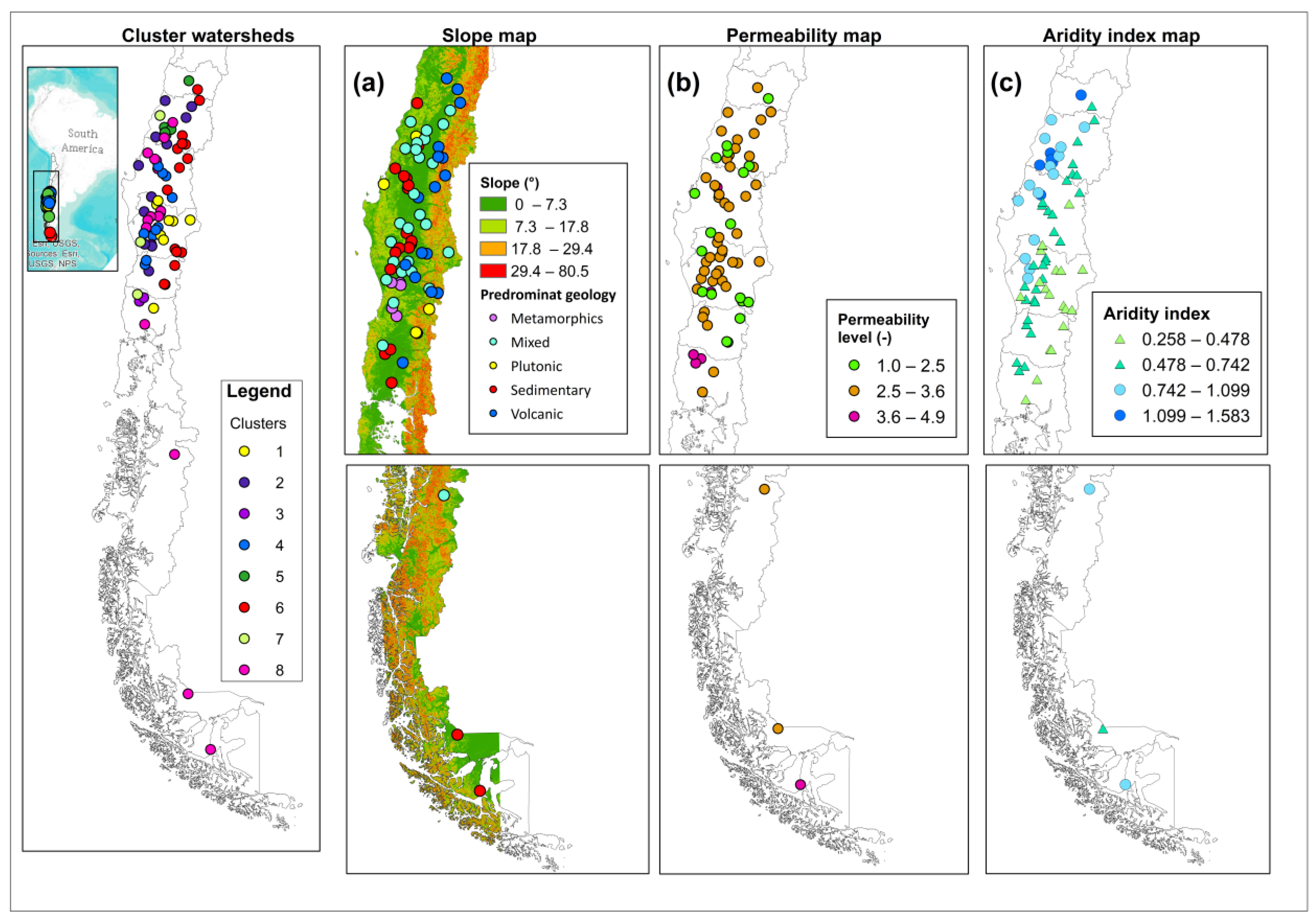
2.1. Study Area

This study used flow records from 72 watersheds located in south-central Chile, between latitudes 30°00″ and 56°30′ S (Figure 1). In general, the selected watersheds did not present significant anthropogenic alterations that would result in changes to recession flows (e.g., dams, canals, artificial storage, etc.).
The selected watersheds present different geological formations (volcanic, plutonic, metamorphic, sedimentary, and mixed) as well as different hydrogeological properties (fractures, porosity, permeability, etc.). These characteristics favor the ability of the watersheds to conduct and transmit water, facilitating interactions among groundwater infiltration, storage, and discharge processes [33,34]. The studied watersheds are monitored on the western slope of the Andes Mountains, the Central Valley, and the Coastal Range.
The period selected for the recession flow analysis comprises 30 years of daily mean flows (1990–2019). The daily mean flow records were obtained from the Catchment Attributes and Meteorology for Large Sample Studies—Chile Dataset (CAMELS-CL) platform, presented by Alvarez-Garreton et al. [35]. This platform includes meteorological (e.g., precipitation and evapotranspiration) and hydrological (e.g., streamflow) data from throughout Chile for each watershed; therefore, post-processing such data (i.e., interpolation) was not necessary. Appendix A presents a table with information on the studied watersheds, while the flow data can be downloaded from the CAMELS-CL platform (https://camels.cr2.cl/, accessed on 15 July 2023.).

2.2. Recession Flow Analysis

The method proposed by Brutsaert and Nieber [25] was used for the recession flow analysis. The snowmelt periods (October–December) of each year of records were removed to obtain periods in which the river streamflow is generated entirely by a groundwater storage-discharge process.
The recession events were obtained from the hydrograph of each basin when dQ/dt was below zero for at least 5 consecutive days until it exceeded zero. To avoid the influence of rapid precipitation-runoff processes, the beginning of the recession period was considered one day after the peak flow.
To determine recession slope b (Equation (1)), the logarithm of the rate of change in flow (dQ/dt) was plotted against the logarithm of average discharge (( Q i + Q i 1 )/2) during the same period. The rate of change (dQ/dt) was calculated using the exponential time-step method (ETS) proposed by Roques et al. [36]. The ETS removes artifacts (errors) resulting from the computation of the rate of change in discharge (dQ/dt). This method differs from the traditional method, in which the time step is constant ( t is equal to t i t i 1 ) , since the time step increases exponentially in each recession event [37]. The time step ( t ) is obtained with an increment m value that is calculated by fitting an exponential function to the recession period. The m value is the total of values in an interval ( t = t i + m t i ). The change rate (dQ/dt) is calculated using the linear least-squares method over the interval ( Q i , Q i + m ; t i , t i + m ) [36]. Slope b was calculated by the log-log linear least-squares method applied to grouped recession data (data bins). The grouped data from an average of log (dQ/dt) and log (Q) considering intervals with 5% of the recession data were obtained.
d Q / d t = a Q b
Parameter b represents the recession regime (or the rate of the decrease in flow over time). A high b value (>1.5) represents a rapid decrease in flows following a precipitation event (fast recession), while a low b value (<1.5) represents a gradual decrease in flows after a precipitation event (slow recession). In other words, in watersheds with low b values, the constant contribution of groundwater to rivers would predominate, blunting the flow decrease. Meanwhile, in watersheds with high b values, a rapid groundwater contribution would predominate and would decrease quickly.

2.3. Clusters

This study used the 8 watershed clusters presented by Parra et al. [28]. These groups were obtained using principal component analysis (PCA) and K-means methods, which were programmed in MATLAB. With the PCA, the coefficients were obtained through covariance matrix decomposition to identify the principal components that capture the greatest data variability. The clusters were obtained via the K-means method, which requires as an input parameter the number of groups (K) to cluster the data. The parameter K represents the number of randomly assigned centroids in each cluster. Via an iterative process, the distances between each centroid and the data are calculated using the squared Euclidian distance. In each iteration, the centroids are recalculated, and all observations are assigned to the nearest cluster or centroid until the assigned data and centroid of each cluster stabilize. The clustering characteristics were the degree of permeability, the mean slope, and the aridity index of each watershed. The degree of permeability was obtained using geological formations and the drainage network of each basin. A permeability value was assigned to each stream/river based on the type of geological formation (5.0 for formations with high permeability, such as fractured geology, and 1.0 for formations with low permeability, such as plutonic geology). Finally, the value of the degree of permeability for the entire watershed was obtained as an average of each stream/river section. The aridity index was obtained as the ratio between mean annual precipitation and mean annual evapotranspiration in each watershed.
Figure 2 shows boxplots with the hydrogeological, morphological, and climate characteristics of the basins for the 8 clusters obtained by Parra et al. [28] (mean elevation, mean slope, degree of permeability, and aridity index). The basins that compose clusters C1 and C6 are located in the Andes Mountains and foothills, with mean elevations ranging from 650 to 1900 m.a.s.l., slopes over 13°, and medium to high permeability (volcanic, plutonic, and mixed geological formations) (see Figure 2a–c). Meanwhile, C3 and C5 are composed of basins monitored in the Central Valley, with mean elevations below 600 m.a.s.l., slopes between 0.7 and 7°, and variable permeability (low, medium, and high) (see Figure 2a–c). Clusters C2, C4, and C8 are composed of a broad group of basins monitored in the Central Valley and Coastal Range (heterogenous clusters). Finally, cluster C7 is composed of basins monitored in the Coastal Range, with mean elevations between 200 and 800 m.a.s.l., slopes between 4 and 11° (Figure 2a,b) and medium-low permeability associated with sedimentary to mixed characteristics.

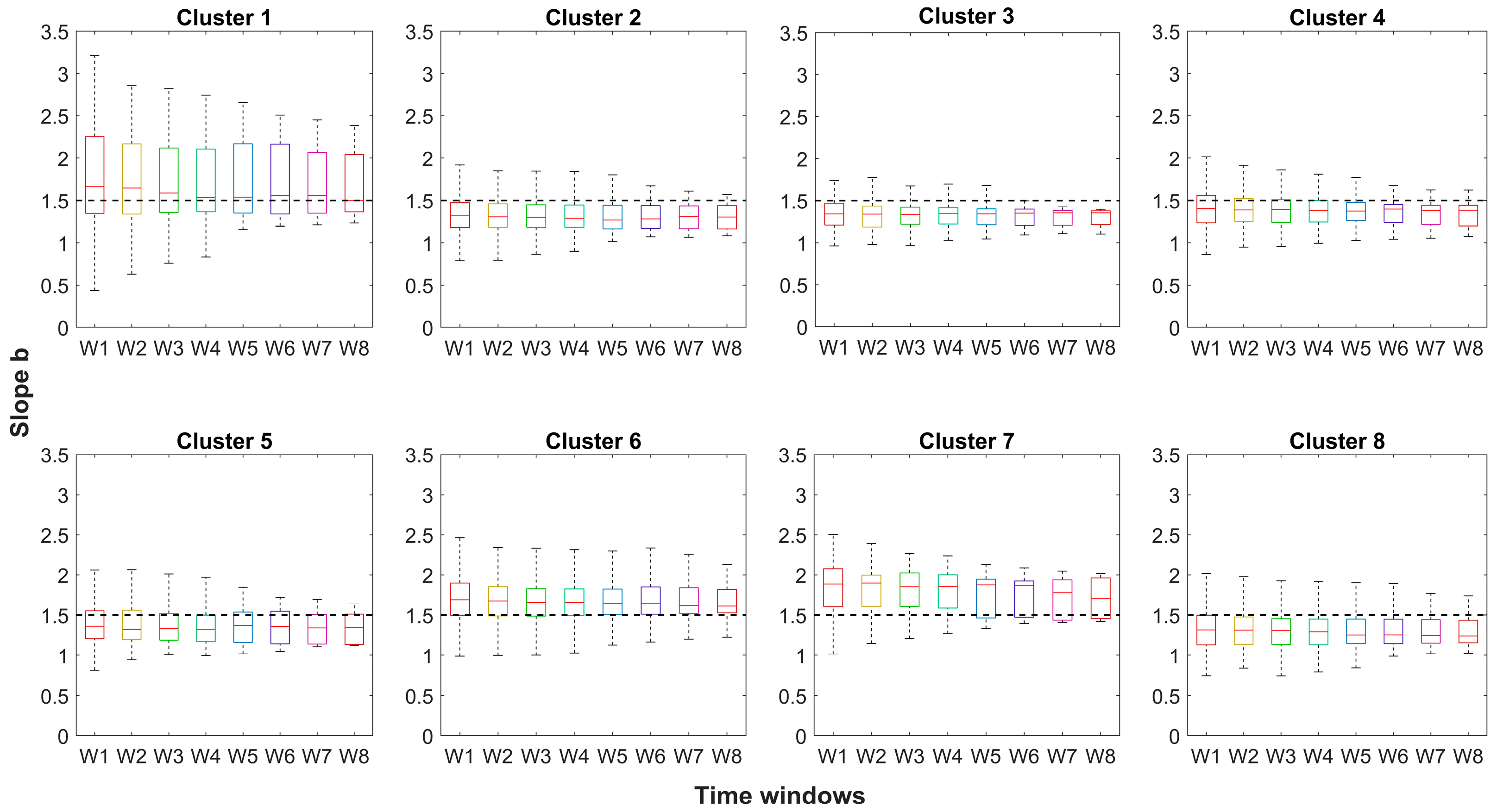
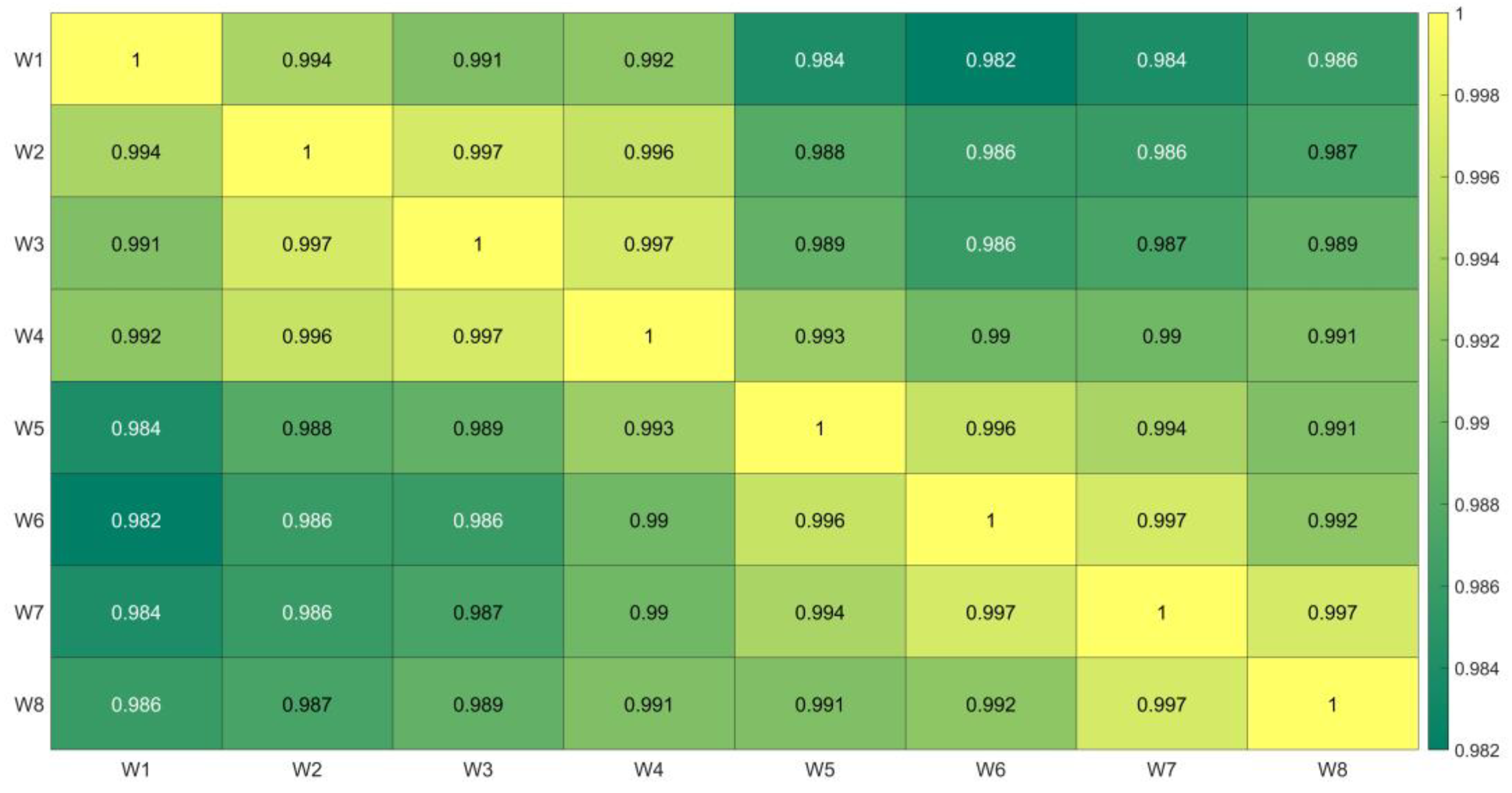
2.4. Estimation of b as a Function of Flow Record Length

To determine the value of b (S-Q process behavior) as a function of flow record length, eight sizes of moving time windows of clustered recession events (point clouds) were analyzed. Time windows of 2 years (w1), 3 years (w2), 4 years (w3), 5 years (w4), 10 years (w5), 15 years (w6), 20 years (w7), and 25 years (w8) were selected to determine a minimum or adequate analysis period, covering long-term processes such as climate variability.

3. Results

Figure 3 shows the results (box-plots) obtained from the recession flow analysis, along with a comparison of results for each time window and cluster, while Figure 4 presents the median slope b obtained from the analysis of each time window.
The results demonstrate a relationship between the recession slope b and the geological and morphological characteristics of the watersheds since the variability of slope b is greater in mountain basins (clusters 1 and 6) than in controlled basins in the central valley (clusters 3 and 5 in Figure 3). In general, Figure 3 shows that the variation (i.e., the size of the box-plot) in the estimation of recession slope b slightly decreases as the size of the time window w increases. Regarding the variation of parameter b, it is observed that in clusters 1, 6, and 7 (formed by watersheds of the Andes Mountains and Coastal Range with a predominance of volcanic and granitic geology), the highest proportion of b values (many b values approximately above the 3rd quartile; see Figure 3) is greater than 1.5. Meanwhile, groups C2, C3, C4, C5, and C8 (formed by watersheds with a predominating sedimentary and mixed geology) present the highest proportion of b values below 1.5 (many values of b below the 3rd quartile; see Figure 3).
Figure 4 shows the median boxplot for each moving window. The median b values in groups C1, C6, and C7 are over 1.5, while in other groups (C2, C3, C4, C5, and C8) the median b value is below 1.5. Therefore, if the median boxplot is considered as the representative slope (b) for each cluster, the size of the window of analysis does not seem to affect the hydrogeological behaviors—that the volcanic and mixed watersheds present a quick recession (rapid drainage) or that the sedimentary and mixed watersheds have a slow recession (slow drainage). In addition, Figure 5 shows the matrix correlation analysis between the median slope b of each watershed in this study obtained from the 8 moving windows. A good fit between the median of each time window is observed (r > 0.98), which indicates that the groundwater behavior may be determined based on the median slope using limited streamflow recession data records (e.g., two-year records).

4. Discussion

In this study, the recession parameter b results obtained from different time windows and watershed clusters were analyzed. In general, if the median of the estimated b values is considered as a representative value of each cluster, the results show that independent of the size of the time window, the watersheds with fast (b > 1.5) or slow drainage hydrogeological behavior (b < 1.5) are consistently identified; however, the smaller the record time window size, the greater the uncertainty in the estimation of recession parameter b (i.e., wider box-plots).
The clusters that show two of the greatest parameter b variability are related to watersheds located in the Andes Mountains (C1 and C6), at elevations over 600 m.a.s.l. and steep slopes above 13° (see Figure 2 and Figure 3). This behavior is linked to the hydrogeological (lava with a high degree of fracturing) and morphological characteristics (steep slopes) of such watersheds (Figure 5). These characteristics favor the interaction of surface water and groundwater [38,39] and, therefore, the behavior of storage-release process dynamics [32]. A similar behavior is observed in the watersheds controlled in the Coastal Range (C7), with mean elevations between 200 and 800 m.a.s.l. and slopes between 4° and 11°, as they also present relatively high variability of slope b. The watersheds located in the Coastal Range present a greater proportion of granitic geology [33] with a high level of soil degradation. This soil presents low permeability [40], which influences runoff generation and the infiltration process [41] and, therefore, the groundwater storage and release relationship represented by parameter b.
The remaining clusters (C2, C3, C4, C5, and C8) show less recession slope variability (narrower boxplots). These watersheds present a major influence of sedimentary and mixed formations, which result in greater stability of flows associated with the aquifer and therefore less b variability. For example, the watersheds of C3 are monitored in the Central Valley of Chile; therefore, they present a greater sedimentary influence. These watersheds present stable behavior, as the median b value remains relatively constant at each time window (see yellow line in Figure 4). This indicates that there is a greater groundwater contribution, maintaining stable flows in rivers in watersheds with sedimentary and mixed geology. The behavior observed in these watersheds is in line with the results presented by Parra et al. [17], who mention that watersheds with sedimentary geology influence residence time, while watersheds with mixed geology present a transitory behavior (fast and slow drainage).
Figure 3 shows that the size of the box decreases as the size of the window under analysis increases, suggesting that the results tend to be more robust with a longer time window under analysis. In addition, if the median of the boxplot is considered as a representative value for the aquifer characterization, a two-year (w1) time window is proven to be enough for almost all clusters (an exception is seen in C1, where more data seems to be necessary to better describe that cluster).
Although the watershed clusters present parameter b variability for the different time windows analyzed, the average hydrogeological behavior (median in Figure 4) is maintained, independent of the size of the time window.
To further analyze if a two-year time window is enough for watershed hydrogeological characterization, the median slope b obtained from 250 aleatoric combinations of two years (non-consecutive) of streamflow recession was plotted (Figure 6). The median was calculated using the slope b values of the watersheds that comprise the cluster obtained from each aleatoric combination of two years. Figure 6 shows that in over 95% of the results, the median hydrogeological behavior for clusters C2, C3, C4, C6, and C8 can be properly obtained from two years of records. On the other hand, it is also observed that clusters C1, C5, and C7, mainly basins with fractured and granitic geology, would need more data records to estimate the hydrogeological behavior of the watersheds.
The results shown indicate that an initial characterization of groundwater system behavior or regime (fast or slow drainage) in watersheds with different geological characteristics can be achieved based on the median of the flow recession curves recorded in two years (not necessarily consecutive years), whether volcanic, sedimentary, plutonic, or mixed geology. On the other hand, watersheds with fractured or granitic geology might need longer records.
Determining hydrogeological behavior via parameter b and its connection to physiographical, geological, and hydrological characteristics allows us to ascertain which watersheds likely have a continuous groundwater contribution to rivers and thus are possibly resilient to climate variability and change [42]. Therefore, recession flow analysis is an adequate tool for providing preliminary results and facilitating the selection of complementary tools suitable for future studies or research on aquifer characterization. In addition, the identification of a minimum time window for groundwater characterization optimizes data collection, decreasing the time and costs associated with groundwater system characterization.
The results obtained from 72 watersheds grouped into eight clusters allow an understanding of the hydrogeological behavior of a group of watersheds with similar geomorphological characteristics. Using clusters allows for more robust conclusions since the findings are related not to a single watershed but rather to a group of watersheds with similar geomorphological characteristics. Small catchments and large basins (100–20,500 km2) were analyzed in this study, covering a wide range of geomorphological features. Therefore, the results could be extrapolated to other areas with similar characteristics. However, validation is recommended, as the clusters obtained are valid for the attributes considered in this study.
The findings of this study conducted in the diverse watersheds of central Chile hold significant importance for understanding the impact of the 15-year drought that has afflicted the region [43]. Lee and Ajami [44] have previously outlined how extended drought periods affect baseflow in rivers across the USA. They elucidate that the decrease in groundwater discharge, stemming from diminished recharge, directly impacts aquifer systems. According to their research, rivers require a long period beyond the duration of the drought to fully recover. Consequently, using a two-year window enables a nuanced understanding of aquifer response to prolonged drought, allowing analysis of changes in recession constants, as demonstrated by Trotter et al. [45]. This observation is particularly noteworthy, especially given recent publications expressing concerns regarding groundwater exploitation in central Chile [46,47,48].

5. Conclusions

This study analyzed recession parameter b based on flow records with different time windows. To this end, watershed clusters with diverse hydrological, geological, and morphological characteristics were used to identify a minimum time period for characterizing the (average) behavior of groundwater storage systems.
The results obtained in this study provide relevant information on the hydrogeological behavior of diverse watersheds, highlighting the importance of considering diverse predominant characteristics and a minimum record length for an adequate characterization. The results show that a size of the time window equal to 25 years for the analysis is sufficient to perform an estimation of parameter b (hydrogeological regime or behavior) in watersheds with different geological, morphological, and hydrological characteristics. Additionally, the results show that an initial characterization of the groundwater system behavior in watersheds of volcanic, sedimentary, plutonic, or mixed geology can be carried out with 2 years of records.
Finally, understanding the behavior of groundwater systems (aquifers) in watersheds with limited hydrogeological records is fundamental for identifying watersheds resilient to climate variability and change. Therefore, the results of this study contribute to practical engineering as they broaden the spectrum of potential data to use to study groundwater systems in watersheds without extensive hydrological and hydrogeological records.

Author Contributions

Conceptualization, V.P. and E.M.; methodology, V.P. and E.M.; validation, V.P. and E.M.; formal analysis, V.P., E.M., J.L.A., Y.M. and R.C.; investigation, V.P. and E.M.; writing—original draft preparation, V.P., E.M., J.L.A., Y.M. and R.C.; writing—review and editing, V.P., E.M. and J.L.A. All authors have read and agreed to the published version of the manuscript.

Funding

This research was funded by the ANID/FONDECYT/3220246 project.

Data Availability Statement

In this study, publicly available datasets were analyzed. These data can be found here: https://camels.cr2.cl/ (accessed on 13 October 2023).

Acknowledgments

The authors thank the General Water Directorate for providing the data used to develop this study, the Center for Climate and Resilience Research (CR)2 for providing data through its https://camels.cr2.cl/ platform (accessed on 15 July 2023), the ANID/FONDECYT/3220246 project, and the CRHIAM Water Center, ANID/FONDAP/15130015 and ANID/FONDAP/1523A0001. The authors also thank Clement Roques, David Rupp, and John Selker for providing the MATLAB code base used in this study.

Conflicts of Interest

Author Yelena Medina was employed by the company Ingeniería EMO-LLS Ltd.a. The remaining authors declare that the research was conducted in the absence of any commercial or financial relationships that could be construed as a potential conflict of interest.

Appendix A

Table A1. Information on the 72 watersheds analyzed in this study.
Gauge
Code
Gauge
Latitude (°)
Gauge
Longitude (°)
Area (km2)Record
Period
Gauge
Code
Gauge
Latitude (°)
Gauge
Longitude (°)
Area (km2)Record
Period
6018001−34.4−71.210231985–20199127001−38.6−72.46501950–2019
9135001−38.9−72.616661929–201910134001−39.6−72.918031969–2019
7336001−36−72.46221945–20197350003−36.3−71.34671964–2019
7343001−35.8−72.14041981–20197354002−36−71.48941986–2019
8220001−36.8−737501960–20198123001−37.2−72.18601924–2019
9102001−38.2−72.98531947–20198130002−36.9−71.62041946–2019
7335002−36.0−722171968–201910343001−40.9−72.73131987–2019
7357002−35.8−71.870791967–20197332001−36.2−7212091967–2019
8343001−37.9−72.44401963–20197335001−36.1−72.116871963–2019
8351001−38−72.44151920–20198124001−36.9−72.416621956–2019
9104001−38.2−72.3941950–20198124002−37.1−72.211481957–2019
9104002−38.2−72.33931987–20198132001−36.9−72.313001956–2019
9106001−38.3−72.42771959–20198135002−36.7−72.545101956–2019
9107001−38.3−72.78541987–20198141001−36.5−72.7104051985–2019
9113001−38.4−72.87101959–20198342001−37.9−72.46881982–2019
8134003−36.7−72.46361985–20199134001−38.9−72.33481985–2019
8317002−37.8−71.91031942–20199140001−38.8−72.955471965–2019
9434001−39.1−72.77701947–20197116001−35.2−71.13671963–2019
10356001−40.7−73.222801986–20197123001−35−7257001987–2019
10362001−40.6−73.14671986–20197330001−36.4−71.65021930–2019
10411002−41.4−73.12531989–20197350001−36.2−71.56691937–2019
9116001−38.6−72.850481929–20197374001−35.5−71.33821961–2019
9433001−39.2−72.71531947–20198323002−37.6−728181941–2019
9436001−39.1−72.93841987–20199437002−39−73.179271990–2019
10121001−39.9−72.86261987–201910364001−40.5−73.356031986–2019
10137001−39.7−735391928–201911302001−45.2−72.119971980–2019
7339001−35.9−72.116371986–20196027001−34.7−70.93491970–2019
7359001−35.6−71.899241975–20197103001−35−70.83541929–2019
8358001−37.7−72.625371964–20198104001−36.7−71.36071966–2019
12582001−53.7−718641970–20199122002−38.5−71.91711986–2019
7383001−35.4−72.2205151985–20199123001−38.4−7213061929–2019
8304001−38.4−71.24671985–20199404001−39−72.216751946–2019
9129002−38.7−72.527561949–201910306001−40.3−72.23091987–2019
9412001−39.4−71.63571968–20199416001−39.3−71.83491971–2019
9414001−39.3−71.813791970–201910102001−39.7−71.83681986–2019
12600001−52−71.95041981–201910304001−40.3−72.317261986–2019

References

  1. Carling, G.T.; Mayo, A.L.; Tingey, D.; Bruthans, J. Mechanisms, timing, and rates of arid región mountain front recharge. J. Hydrol. 2012, 428–429, 15–31. [Google Scholar] [CrossRef]
  2. Kao, Y.H.; Liu, C.W.; Wang, S.W.; Lee, C.H. Estimating mountain block recharge to downstream alluvial aquifers from standard methods. J. Hydrol. 2012, 426–427, 93–102. [Google Scholar] [CrossRef]
  3. Marchant, B.P.; Cuba, D.; Brauns, B.; Bloomfield, J.P. Temporal interpolation of groundwater level hydrographs for regional drought analysis using mixed models. Hydrogeol. J. 2022, 30, 1801–1817. [Google Scholar] [CrossRef]
  4. Marti, E.; Leray, S.; Villela, D.; Maringue, J.; Yáñez, G.; Salazar, E.; Poblete, F.; Jimenez, J.; Reyes, G.; Poblete, P.; et al. Unravelling geological controls on groundwater flow and surface water-groundwater interaction in mountain systems: A multi-disciplinary approach. J. Hydrol. 2023, 623, 129786. [Google Scholar] [CrossRef]
  5. Srzić, V.; Lovrinović, I.; Racetin, I.; Pletikosić, F. Hydrogeological Characterization of Coastal Aquifer on the Basis of Observed Sea Level and Groundwater Level Fluctuations: Neretva Valley Aquifer, Croatia. Water 2020, 12, 348. [Google Scholar] [CrossRef]
  6. Killian, C.D.; Asquith, W.H.; Barlow, J.R.B.; Bent, G.C.; Kress, W.H.; Barlow, P.M.; Schmitz, D.W. Characterizing groundwater and surface-water interaction using hydrograph-separation techniques and groundwater-level data throughout the Mississippi Delta, USA. Hydrogeol. J. 2019, 27, 2167–2179. [Google Scholar] [CrossRef]
  7. Wu, R.S.; Hussain, F.; Lin, Y.C.; Yeh, T.Y.; Yu, K.C. Characterization of Regional Groundwater System Based on Aquifer Response to Recharge–Discharge Phenomenon and Hierarchical Clustering Analysis. Water 2021, 13, 2535. [Google Scholar] [CrossRef]
  8. Sandoval, E.; Baldo, G.; Núñez, J.; Oyarzún, J.; Fairley, J.P.; Ajami, H.; Arumí, J.L.; Aguirre, E.; Maturana, H.; Oyarzún, R. Groundwater recharge assessment in a rural, arid, mid-mountain basin in North-Central Chile. Hydrol. Sci. J. 2018, 63, 1873–1889. [Google Scholar] [CrossRef]
  9. Blarasin, M.; Matiatos, I.; Cabrera, A.; Lutri, V.; Giacobone, D.; Becher Quinodoz, F.; Matteoda, E.; Eric, C.; Felizzia, J.; Giuliano Albo, J. Characterization of groundwater dynamics and contamination in an unconfined aquifer using isotope techniques to evaluate domestic supply in an urban area. J. S. Am. Earth Sci. 2021, 10, 103360. [Google Scholar] [CrossRef]
  10. Ghani, J.; Ullah, Z.; Nawab, J.; Iqbal, J.; Waqas, M.; Ali, A.; Almutairi, M.H.; Peluso, I.; Mohamed, H.R.H.; Shah, M. Hydrogeochemical Characterization, and Suitability Assessment of Drinking Groundwater: Application of Geostatistical Approach and Geographic Information System. Front. Environ. Sci. 2022, 10, 874464. [Google Scholar] [CrossRef]
  11. Tajwar, M.; Uddin, A.; Lee, M.K.; Nelson, J.; Zahid, A.; Sakib, N. Hydrochemical Characterization and Quality Assessment of Groundwater in Hatiya Island, Southeastern Coastal Region of Bangladesh. Water 2023, 15, 905. [Google Scholar] [CrossRef]
  12. Christensen, C.W.; Hayashi, M.; Bentley, L.R. Hydrogeological characterization of an alpine aquifer system in the Canadian Rocky Mountains. Hydrogeol. J. 2020, 28, 1871–1890. [Google Scholar] [CrossRef] [PubMed]
  13. Sendrós, A.; Himi, M.; Lovera, R.; Rivero, L.; Garcia-Artigas, R.; Urruela, A.; Casas, A. Geophysical Characterization of Hydraulic Properties around a Managed Aquifer Recharge System over the Llobregat River Alluvial Aquifer (Barcelona Metropolitan Area). Water 2020, 12, 3455. [Google Scholar] [CrossRef]
  14. Chen, H.; Teegavarapu, R.S.V. Comparative Analysis of Four Baseflow Separation Methods in the South Atlantic-Gulf Region of the U.S. Water 2020, 12, 120. [Google Scholar] [CrossRef]
  15. Zhang, Y.; He, Y.; Mu, X.; Jia, L.; Li, Y. Base-flow segmentation and character analysis of the Huangfuchuan Basin in the middle reaches of the Yellow River, China. Front. Environ. Sci. 2022, 10, 831122. [Google Scholar] [CrossRef]
  16. Lin, K.; Yeh, H. Baseflow recession characterization and groundwater storage trends in northern Taiwan. Hydrol. Res. 2017, 48, 1745–1756. [Google Scholar] [CrossRef]
  17. Parra, V.; Arumí, J.L.; Muñoz, E.I. Characterization of the Groundwater Storage Systems of South-Central Chile: An Approach Based on Recession Flow Analysis. Water 2019, 11, 1506. [Google Scholar] [CrossRef]
  18. Yan, H.; Hu, H.; Liu, Y.; Tudaji, M.; Yang, T.; Wei, Z.; Chen, L.; Ali Khan, M.Y.; Chen, Z. Characterizing the groundwater storage–discharge relationship of small catchments in China. Hydrol. Res. 2022, 53, 782–794. [Google Scholar] [CrossRef]
  19. Yi, W.; Feng, Y.; Liang, S.; Kuang, X.; Yan, D.; Wan, L. Increasing annual streamflow and groundwater storage in response to climate warming in the Yangtze River source region. Environ. Res. 2021, 16, 084011. [Google Scholar] [CrossRef]
  20. Mouakoumbat, N.; Gampio, U.; Nkaya, G.; Ebotehouna, C.; Ondon, A.; Niere, R. Hydrogeological Characterization and Approach to a Conceptual Model of the Aquifer of the Cuvette Basin, Republic of Congo. Int. J. Geosci. 2022, 13, 997–1023. [Google Scholar] [CrossRef]
  21. Chenini, I.; Msaddek, M.H.; Dlala, M. Hydrogeological characterization and aquifer recharge mapping for groundwater resources management using multicriteria analysis and numerical modeling: A case study from Tunisia. J. Afr. Earth Sci. 2019, 154, 59–69. [Google Scholar] [CrossRef]
  22. Fuentes-Arreazola, M.A.; Ramírez-Hernández, J.; Vázquez-González, R. Hydrogeological Properties Estimation from Groundwater Level Natural Fluctuations Analysis as a Low-Cost Tool for the Mexicali Valley Aquifer. Water 2018, 10, 586. [Google Scholar] [CrossRef]
  23. de Barros, F.P.J.; Ezzedine, S.; Rubin, Y. Impact of hydrogeological data on measures of uncertainty, site characterization and environmental performance metrics. Adv. Water Resour. 2012, 36, 51–63. [Google Scholar] [CrossRef]
  24. Cooper, M.; Zhou, T. baseflow: A MATLAB and GNU Octave package for baseflow recession analysis. J. Open Source Softw. 2023, 8, 5492. [Google Scholar] [CrossRef]
  25. Brutsaert, W.; Nieber, J.L. Regionalized drought flow hydrographs from a mature glaciated plateau. Water Resour. Res. 1977, 13, 637–643. [Google Scholar] [CrossRef]
  26. Kirchner, J.W. Catchments as simple dynamical systems: Catchment characterization, rainfall-runoff modeling, and doing hydrology backward. Water Resour. Res. 2009, 45, W02429. [Google Scholar] [CrossRef]
  27. Ye, S.; Li, H.; Huang, M.; Ali, M.; Leng, G.; Leung, L.R.; Sivapalan, M. Regionalization of subsurface stormflow parameters of hydrologic models: Derivation from regional analysis of streamflow recession curves. J. Hydrol. 2014, 519, 670–682. [Google Scholar] [CrossRef]
  28. Parra, V.; Muñoz, E.; Arumí, J.L.; Medina, Y. Analysis of the Behavior of Groundwater Storage Systems at Different Time Scales in Basins of South Central Chile: A Study Based on Flow Recession Records. Water 2023, 15, 2503. [Google Scholar] [CrossRef]
  29. Santos, A.C.; Portela, M.M.; Rinaldo, A.; Schaefli, B. Estimation of streamflow recession parameters: New insights from an analytic streamflow distribution model. Hydrol. Process. 2019, 33, 1595–1609. [Google Scholar] [CrossRef]
  30. Karlsen, R.H.; Bishop, K.; Grabs, T.; Ottosson-Löfvenius, M.; Laudon, H.; Seibert, J. The role of landscape properties, storage and evapotranspiration on variability in streamflow recessions in a boreal catchment. J. Hydrol. 2019, 570, 315–328. [Google Scholar] [CrossRef]
  31. Tashie, A.; Pavelsky, T.; Band, L.E. An empirical reevaluation of streamflow recession analysis at the continental scale. Water Resour. Res. 2020, 56, e2019WR025448. [Google Scholar] [CrossRef]
  32. Li, H.; Ameli, A. A statistical approach for identifying factors governing streamflow recession behavior. Hydrol. Process. 2022, 36, e14718. [Google Scholar] [CrossRef]
  33. SERNAGEOMIN. Mapa Geológico de Chile: Versión Digital. Servicio Nacional de Geología y Minería; Publicación Geológica Digital: Santiago, Chile, 2003. [Google Scholar]
  34. Voeckler, H.; Allen, D.M. Estimating regional-scale fractured bedrock hydraulic conductivity using discrete fracture network (DFN) modeling. Hydrogeol. J. 2012, 20, 1081–1100. [Google Scholar] [CrossRef]
  35. Alvarez-Garreton, C.; Mendoza, P.A.; Boisier, J.P.; Addor, N.; Galleguillos, M.; Zambrano-Bigiarini, M.; Lara, A.; Puelma, C.; Cortes, G.; Garreaud, R.; et al. The CAMELS-CL dataset: Catchment attributes and meteorology for large sample studies—Chile dataset. Hydrol. Earth Syst. Sci. 2018, 22, 5817–5846. [Google Scholar] [CrossRef]
  36. Roques, C.; Rupp, D.; Selker, J. Improved streamflow recession parameter estimation with attention to calculation of −dQ/dt. Adv. Water Resour. 2017, 108, 29–43. [Google Scholar] [CrossRef]
  37. Kim, M.; Bauser, H.H.; Beven, K.; Troch, P.A. Time-variability of flow recession dynamics: Application of machine learning and learning from the machine. Water Resour. Res. 2023, 59, e2022WR032690. [Google Scholar] [CrossRef]
  38. Parra, V.; Muñoz, E.; Arumí, J.L.; Paredes, J. Análisis de la interacción de aguas superficiales y subterráneas en una cuenca volcánica andina, Chile. Tecnol. Cienc. Agua 2020, 11, 303–320. [Google Scholar] [CrossRef]
  39. Taucare, M.; Viguier, B.; Daniele, L.; Heuser, G.; Arancibia, G.; Leonardi, V. Connectivity of fractures and groundwater flows analyses into the Western Andean Front by means of a topological approach (Aconcagua Basin, Central Chile). Hydrogeol. J. 2020, 28, 2429–2438. [Google Scholar] [CrossRef]
  40. Hafidz, A.; Kinoshita, N.; Yasuhara, H. Effect of permeants on fracture permeability in granite under hydrothermals conditions. Rock Mech. Bull. 2022, 1, 100007. [Google Scholar] [CrossRef]
  41. Uribe, H.; Arumí, J.L.; González, M.; Salgado, L. Groundwater recharges using hydrological balances in the central drylands of Chile. Ingeniería Hidráulica en México 2003, 18, 17–28. [Google Scholar]
  42. Jachens, E.R.; Roques, C.; Rupp, D.E.; Selker, J.S. Streamflow recession analysis using water height. Water Resour. Res. 2020, 56, e2020WR027091. [Google Scholar] [CrossRef]
  43. Garreaud, R.D.; Boisier, J.P.; Rondanelli, R.; Montecinos, A.; Sepúlveda, H.H.; Veloso-Aguila, D. The Central Chile Mega Drought (2010–2018): A climate dynamics perspective. Int. J. Climatol. 2020, 40, 421–439. [Google Scholar] [CrossRef]
  44. Lee, S.; Ajami, H. Comprehensive assessment of baseflow responses to long-term meteorological droughts across the United States. J. Hydrol. 2023, 626 Pt A, 130256. [Google Scholar] [CrossRef]
  45. Trotter, L.; Saft, M.; Peel, M.C.; Fowler, K.J.A. Recession constants are non-stationary: Impacts of multi-annual drought on catchment recession behaviour and storage dynamics. J. Hydrol. 2024, 630, 130707. [Google Scholar] [CrossRef]
  46. Jódar, J.; Urrutia, J.; Herrera, C.; Custodio, C.; Martos-Rosillo, S.; Lambán, L.J. The catastrophic effects of groundwater intensive exploitation and Megadrought on aquifers in Central Chile: Global change impact projections in water resources based on groundwater balance modeling. Sci. Total Environ. 2024, 914, 169651. [Google Scholar] [CrossRef] [PubMed]
  47. Taucare, M.; Viguier, B.; Figueroa, R.; Daniele, L. The alarming state of Central Chile’s groundwater resources: A paradigmatic case of a lasting overexploitation. Sci. Total Environ. 2024, 906, 167723. [Google Scholar] [CrossRef]
  48. Alvarez-Garreton, C.; Boisier, J.P.; Garreaud, R.; González, J.; Rondanelli, R.; Gayó, E.; Zambrano-Bigiarini, M. HESS Opinions: The unsustainable use of groundwater conceals a “Day Zero”. Hydrol. Earth Syst. Sci. 2024, 28, 1605–1616. [Google Scholar] [CrossRef]
Figure 1. Locations of the watersheds used in the study area and their hydrological and geomorphological characteristics. The predominant slope map (a), degree of permeability (b), and aridity index (c) of each watershed are shown.
Water 16 01741 g001
Figure 2. Cluster characteristics. The mean elevation (a), mean slope (b), degree of permeability (c), and aridity index (d) of each cluster are also shown.
Water 16 01741 g002
Figure 3. Boxplots with values of recession parameter b obtained for different watershed groups (clusters). w1, w2, w3, w4, w5, w6, w7, and w8 correspond to moving windows of 2 years, 3 years, 4 years, 5 years, 10 years, 15 years, 20 years, and 25 years, respectively.
Water 16 01741 g003
Figure 4. Median slope b values of each cluster obtained from the different time windows. The dashed line represents the limit value of b for fast drainage (b > 1.5) and slow drainage processes (b < 1.5). w1, w2, w3, w4, w5, w6, w7, and w8 correspond to moving windows of 2 years, 3 years, 4 years, 5 years, 10 years, 15 years, 20 years, and 25 years, respectively.
Water 16 01741 g004
Figure 5. The correlation matrix between each watershed’s median slope b values from the 8 time windows.
Water 16 01741 g005
Figure 6. Median slope b values of two-year combinations. The dashed line represents the limit value of b for fast drainage (b > 1.5) and slow drainage processes (b < 1.5).
Water 16 01741 g006
Disclaimer/Publisher’s Note: The statements, opinions and data contained in all publications are solely those of the individual author(s) and contributor(s) and not of MDPI and/or the editor(s). MDPI and/or the editor(s) disclaim responsibility for any injury to people or property resulting from any ideas, methods, instructions or products referred to in the content.

