Irrigation Performance Assessment, Opportunities with Wireless Sensors and Satellites

Abstract

Irrigation is an essential component of our food production system and a large user of freshwater. Pressure on irrigated agriculture is likely to increase with growing populations and climate uncertainty. Efforts to ensure sustainable water use in this sector have had mixed results. Some of these efforts have been used in the interest of political or financial gain. The situation is complicated by the vulnerability of irrigating farmers, locally within irrigation schemes and in the global agricultural supply chain. An opportunity exists in the form of increasing the accessibility of open-source remote sensing products and wireless sensor networks. Irrigating farmers can define and assess their irrigation performance at different spatial and temporal scales. A review of irrigation performance assessment approaches and the available products and sensors is presented. Potential implementations for sensing and monitoring, as well as irrigation performance, are presented. The possibilities at different time scales and the influence on performance of different groups within the irrigation scheme are discussed. The particular circumstances of specific irrigation schemes need to be assessed with a cost–benefit analysis. The implementation of irrigation performance analysis tools should be led by irrigating farmers, as it directly impacts this group.

1. Introduction

Irrigation and human development have historically been inextricably linked. Ancient irrigation systems allowed settlements to grow in otherwise inhospitable and arid places, such as deserts on the dry coast of Peru [1]. Today, irrigated agriculture provides 40 percent of our food on 20 percent of the cultivated land, a major contribution to agriculture and accounting for 70 percent of freshwater withdrawals [2]. We are now more than ever bound to irrigated food production, as the global population is set to reach 9.7 billion in the next 30 years [3]. This is amid increasing climate uncertainty and potential water scarcity.

With such predictions, ensuring sustainable and optimal water use has a high importance. This is stated in the United Nations’ Sustainable Development Goals (UNSDG). UNSDG 6 target 6.4 aims to “… substantially increase water-use efficiency across all sectors and ensure sustainable withdrawals and supply of freshwater to address water scarcity …” [4]. Several other UNSDG’s are also linked to irrigation, covering sustainable agriculture, climate change and the protection of terrestrial ecosystems. Irrigation performance has often and in many contexts been attributed to measures of irrigation efficiency, which in some cases have been misunderstood or misused [5,6]. Additionally, irrigation performance terms have been used in political discourse and in the marketing of irrigation equipment by companies. Claims by commercial interests that certain types of high-tech installations can achieve high efficiency compared to the low efficiency of current practices are difficult to evaluate in field conditions within the wider setting of irrigation schemes [7,8]. These terms should be used cautiously, as they hold significant power to influence the livelihoods of potentially vulnerable groups [9].

The majority of farms are family run enterprises [10]. Typically, they do not have at their disposal the capital and financial flexibility of large agro-industrial enterprises. A farmer investing in advanced sprinkler or drip systems may be able to more effectively use their allocated water and labor. This can lead to farmers increasing their cultivated area or moving to higher value cash crops. However, the nested and embedded nature of irrigation systems and water flows mean that what is true for the part is not necessarily true for the whole. An example is the impact of the head-end/tail-end effect, where farmers further away from the head-end of the irrigation supply are at a significant disadvantage compared to farmers closer to the head-end. At a global scale, the potential for further exploitation of existing inequities is apparent, as international investments are undertaken in the name of development and food security but can be qualified as a form of neo-colonialism [11]. Seckler foresaw a shift towards the trading of crop water content, potentially increasing scrutiny on irrigation performance [12]. The increasing accessibility of sensor technology through open-source remote sensing (OSRS) and wireless sensor networks (WSN) presents opportunities for farmers, and the organizational structures they make up within irrigation schemes, to define and assess the performance of their irrigation.

In this paper, the common definitions of irrigation performance and approaches to assessing irrigation performance in large irrigation schemes are reviewed. In Section 2, irrigation performance will be discussed, first looking at the most important elements in the history of its development. Combining this historical perspective with important recent developments, a water performance mosaic capturing the multi-scale nature of irrigation is used. In Section 3, key variables in quantifying irrigation performance are identified, and the available methods in OSRS and WSN for sampling these variables are reviewed. Options for sensing strategies are discussed in Section 3.3.

2. Irrigation Performance

The performance of irrigation has for a long time and in many different contexts been reduced to an oversimplified measure of efficiency. Efficiency in its strict definition is the amount of useful output of a process, such as water for crop growth, relative to the total input to the process, such as water supplied. In its initial form over 100 years ago, the useful output was first identified as the ‘duty of water’ and was directly linked to the amount of water needed to grow a particular crop [13]. This gave rise to the concepts of irrigation conveyance and field application efficiencies. Israelsen et al. first applied water-application efficiencies as a response to rising land and water costs, with the aim of optimizing use [14]. This has led to long-lasting debates on the suitable application of specific terms, the development of new ones, and their reformulation. Often, definitions have been linked to the differing perspectives of the various actors. Each actor usually looking at the irrigation scheme at a different scale, such as the farm or irrigation system in particular or the wider water resources system.

Significant developments in irrigation performance assessment included the differentiation between classical irrigation efficiency, $E_C$, and effective irrigation efficiency, $E_E$ and the development of the fractions concept [13,15,16]. These concepts have not only shaped research in irrigation and the assessment of its performance but the viewpoints of policy makers and the public. $E_C$ focuses narrowly on the technical infrastructural path from resource to useful water for the crop. $E_E$ takes a wider perspective, including the water streams parallel to the irrigation infrastructure, for example the outflow from the tail end of an over-irrigated field back into the canal, to be potentially reused by downstream fields. Identifying water streams and classifying them resulted in fractions within the overall flow from the water resource to the crop and beyond. The original intent of the introduction of fractions into the discourse on irrigation performance was as a means to replace irrigation efficiency, as indicated by the title of the article by [13]. However, this concept helps to fill in the picture of irrigation performance by classifying the different streams regarding their value to the system.

A more recent outcome of these debates has been the irrigation efficiency matrix (IEM) as developed by [17]. This scale-based framework is an extensive and in-depth tool for the solid placement of irrigation efficiency in the realm of water management. The scales of the IEM capture the different levels at which important water interactions take place, these are as follows:

• Sub-field;
• Field, orchard, farm, tertiary irrigation unit;
• Total irrigation system;
• Catchment, basin, aquifer, multiple irrigation systems;
• Supra/inter/national, trans-boundary basin, irrigated sector, markets and firms.

Although the fraction approach and IEM are logical developments, they are rather complex and difficult to apply in practice, especially when compared to the earlier definitions of irrigation performance. Some fractions are difficult to measure and quantify and can only be described and the order of their magnitude estimated. From this introduction, it should be understood that irrigation performance in this article encompasses the efficient and sustainable use of water and soils for biomass production. With this premise, the current section sets up a model for the conceptualization of irrigation performance and reviews its components.

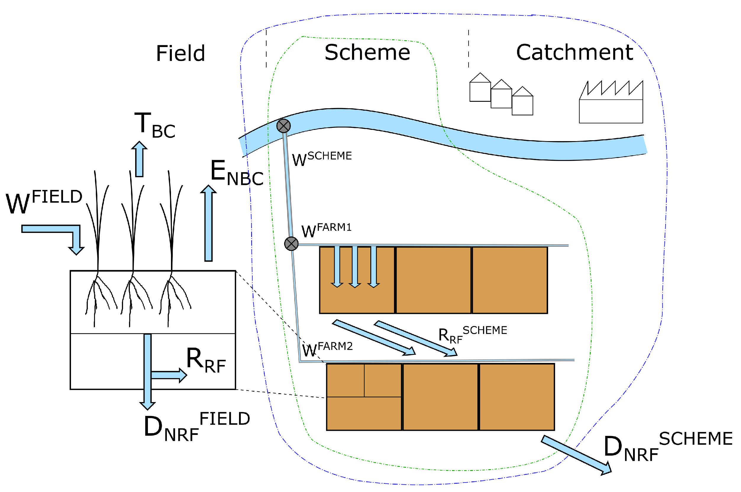
2.1. Performance Analysis Scheme

To capture the nested and embedded nature of irrigation systems and identify the required components for effective performance analysis, a conceptualization of irrigation is needed. A combination of two typical representations of irrigation has been chosen. Illustrations of cropping systems have often resembled one or both of these models. These two models are used here based on their illustration and definition by [6]. These authors described the two models as paradigms in irrigation efficiency assessment. Basin allocated irrigation efficiency (BAIE), also called the block model, has been used to illustrate irrigation water flows in individual fields and farms. While it lends itself well to simple and clear representations of field water balance, it is well suited to illustrating farms that control their own water resource, such as a private well in or proximal to the field. With socialized localized irrigation efficiency (SLIE), or bifurcating model, the farmers share a common water resource as part of a larger-scale irrigation system. The network is described spatially with the inclusion of offtake points, bifurcations of supply, and the relative positioning of fields and farms. It may be constructed from canals, pipes, or a combination of both, but most importantly, the spatial relationships within the system and the nature of water flowing through and around it are described.

These models complement one another and were described both individually and with their nested characteristics by [6]. In this article, we follow on from this and include three of the previously listed scales outlined in the IEM, namely 1. field, 2. scheme, and 3. catchment, to provide different perspectives for assessing the performance of irrigation. These scales were selected as they represent tangible management levels in terms of irrigation performance assessment for the purpose of this article. Figure 1 illustrates the scales discussed relative to the combined models and the category of each water stream as a fraction.

Assessing irrigation performance does not solely rest on technological or organizational requirements. Certain aspects of irrigation schemes, such as supply organization, maintenance condition, policy and regulation, technical expertise, and equipment and infrastructure development level, affect the ability to implement management, organizational, or technological changes [18]. While important, these elements are not explicitly discussed in this section, as they are outside the scope of this article. Using Figure 1, we can position the component water streams across scales and derive sensing requirements.

2.2. Performance Indicators

Performance indicators for irrigation assessment require a combination of flexibility and robustness. They should be applicable across a variety of different irrigation systems and capture a system’s performance in a standardized and comparable manner. In this subsection, indicators of particular importance and interest for the assessment of irrigation performance are discussed.

Combining the scales of an irrigation scheme with the performance indicators leads to the formulation of a mosaic of water values. However, the irrigation performance issues faced by farmers span entire seasons when considering biomass productivity, but come down to days and hours when concerns about irrigation timing and supply discharges arise, and even minutes when the timing of a specific irrigation dose to a field is discussed. It is therefore clear that temporal scales in the application of performance indicators must also be carefully considered. This section details the widely used irrigation performance indicators.

2.2.1. Classical Irrigation Efficiency

The exact definition of $E_C$ has varied according to different perspectives. A generally accepted definition is the ratio of water consumed by a crop relative to the water applied, delivered, or diverted [16]. Considering fractions, the consumption of water can be classified as either beneficial or non-beneficial; as illustrated in Figure 1, with a beneficial consumption being plant transpiration while a non-beneficial one being soil evaporation. The long-standing use of crop evapotranspiration, $E{T}_C$, based on the FAO method detailed by Allen et al. for the estimation of irrigation demand, further discussed in Section 3, makes the decoupling of the evaporation and transpiration terms complex, not only in measurement but also analytically [19]. Considering the impacts of stress and other factors on evapotranspiration affects the $E{T}_C$, which is replaced by actual evapotranspiration, $E{T}_A$. $E{T}_A$ is used in the numerator, as shown in Equation (1). Equation (1) can be adjusted to different spatial scales such as field, farm, and scheme, as long as both the numerator and the denominator, W, are adjusted to the proper scale. It is recommended to subtract effective precipitation, $P_e$, which contributes to the watering of the crop, from the evapotranspiration term.

$E_C$ has often been broken down into the two component parts of conveyance efficiency, $E_{CONV}$, and application efficiency, $E_{APP}$, as shown in Equation (2). This decoupling can be a way of separating the farmers’ responsibilities from those of the scheme managers. The supply of water to the farm and associated $E_{CONV}$ are the domain of the scheme engineers and managers. The application of water to the field and what is actually done with the water on the farm, $E_{APP}$, is that of the farmer [5]. $E_{APP}$ and $E_{CONV}$ can be applied from the farm scale up to the wider scheme, as the conveyance of water to different individual users is taken into account. $E_C$ and its components are performance indicators with an infrastructure-centric perspective. They can be summarized as the ratio of a beneficial or intended use of water of a process to the total amount of water dedicated to the process. It is important to note that beneficial uses of water from irrigation include other elements, as is explained in the next section on $E_E$.

$$E_C=\frac{E{T}_A-P_e}{W}$$

(1)

$$E_C=E_{CONV}\ast E_{APP}$$

(2)

$$E_{CONV}=\frac{W}{W_{delivered}}$$

(3)

$$E_{APP}=\frac{E{T}_A-P_e}{W_{delivered}}$$

(4)

2.2.2. Effective Irrigation Efficiency

$E_E$ was introduced by Keller and Keller to overcome the limitations of $E_C$ in the wider context of the water resources [15]. Compared to the classical method, $E_E$ broadened the field of view to more effectively capture the potential reuse of water within an irrigation scheme. This perspective incorporates both the quantity and quality of the water by considering the leaching requirement, $LR$. As water is removed to the atmosphere through evaporation or transpiration it leaves behind salts, which accumulate in the remaining water and soil and need to be leached out of the root zone. $LR$ is an amount of water dependent on the crop’s tolerance to salinity, the soil type, and the quality of the irrigation water that is provided in addition to the crop requirement.

$E_E$ is a ratio of the irrigation water beneficially consumed in the scheme, similar to the numerator in Equation (1), to the effective supply, as shown in Equation (5) [15,20]. The effective supply is based on the difference between the effective inflow, $W_{eI}$, and effective outflow, $W_{eO}$, of the scheme. $W_{eI}$ and $W_{eO}$ are dependent on $LR$ and the in- and outflows to the scheme, V, as indicated in Equation (6). This performance indicator is intended to capture the possibility that a certain amount of water re-use can occur in irrigation schemes. This may be when a farmer closer to the source of water over-irrigates their field and the excess water is then available to the crop of another farmer downstream.

$$E_E=\frac{E{T}_A}{W_{eI}-W_{eO}}$$

(5)

$$\begin{array}{cc}{W}_{eI}=(1-L{R}_I)V_I \hfill & \hfill W_{eO}=(1-L{R}_O)V_O\end{array}$$

(6)

2.2.3. Relative Irrigation Supply

Relative irrigation supply, $RIS$, is a measure of the effectiveness of water delivery and indicates how adequately the irrigation supply system is meeting demand [5]. $RIS$ can be defined alongside the relative water supply, $RWS$ [21]. $RWS$ is a similar indicator to $RIS$, but they differ in the inclusion of non-irrigation water supply. $RWS$ includes the total water supply by including effective precipitation in W, whereas $RIS$ focuses on the relation between supplied irrigation and the crop water requirement, $CWR$. $RIS$ is defined in Equation (7).

$RIS$ can be applied from farm up to scheme scale and adjusted to assess the performance of specific areas of the scheme. An appropriate time scale needs to be applied, as the $CWR$ and W must cover the same temporal window, and this may be daily, weekly, or up to seasonal. An ideal value for this indicator is as close to 1 as possible, as greater than 1 means over-irrigation or ineffective application. Much smaller than 1 indicates a $CWR$ that cannot be satisfied with the current supply. Under water shortage conditions a lower $RIS$ can be targeted, for example around 0.7, to achieve optimal water productivity.

$$RIS=\frac{W}{CWR}$$

(7)

2.2.4. Water Delivery Performance

The water delivery performance, $WDP$, compares the intended amount of water to be delivered by a conveyance system, $W_{intended}$, with the actual amount delivered, $W_{actual}$, focusing on the operation of the scheme in terms of the quality of water delivery service [5]. This indicator may be based on volume or on average discharge over a specific period of time [22]. Both variations of the basic indicator detailed in Equation (8) assess the performance of the conveyance system. The two types are complementary. The focus on discharge can provide more insight into the hydraulic control capacity of the scheme, while the focus on volume will inform about whether the supply is sufficient and planning has been appropriately carried out to meet demand. Similarly to $RIS$, values in excess of 1 indicate excess supply or improper planning of water allocation.

$$WDP=\frac{W_{actual}}{W_{intended}}$$

(8)

2.2.5. Water Productivity

Water productivity, $WP$, makes a link between water management and the actual outputs of the irrigation scheme. It is the ratio of physical or economic production to the amount of water withdrawn, applied, or consumed. The time scale is constrained to at least one or more growing seasons, as the completion of one growing cycle is required but the spatial scale is more fluid. Along with this fluidity, different stakeholders also have changing interpretations of $WP$.

Plant physiologists assessing energy conversion are interested in $WP$ at the scale of individual plants, while water managers and hydrologists look at the basin scale, with other stakeholders at each level in between these extremes [16]. As in Equation (9), $WP$ can be assessed from field to scheme scale with the numerator, P, representing agricultural production as either physical dry product or financial revenue, and the denominator, W, representing water used as either withdrawn, applied, or consumed. It should be noted that $WP$ is influenced by a number of variables that change among farms, such as seed selection, planting dates, soil, weeding, fertilization, and pest control [7]. $WP$ is higher when $RIS$ is lower than 1 and is, depending on the crop, soil, and climate, often optimal for a $RIS$ in the order of magnitude of 0.7.

$$WP=\frac{P_{dryproduct/revenue}}{W_{withdrawn/applied/consumed}}$$

(9)

A number of other indicators have been developed and applied for the assessment of irrigation performance. A comprehensive summary of indicators dealing both with the technical and organizational aspects of irrigation was compiled by [22]. Fifteen irrigation performance indicators were considered by Zafar et al., and these authors assessed the maturity and acceptance of the indicators in the scientific community [23].

2.3. Mosaic of Irrigation Performance

Van Halsema and Vincent argued the need for a $WP$ value mosaic to capture the multi-scale aspect of this indicator [5]. The approach should include the nested and embedded scales of the operation of irrigation, from the field level up to trans-boundary watersheds. The specific and appropriate scales at which performance indicators can be applied and the form they take need to be specified. A general schematic describing this is the mosaic of irrigation performance illustrated in

Table 1. Mosaic of irrigation performance. $E_C$ is classical irrigation efficiency as in Section 2.2.1, $E_E$ is effective irrigation efficiency as in Section 2.2.2, $E_{APP}$ is application efficiency as in Section 2.2.1, $E_{CONV}$ is conveyance efficiency as in Section 2.2.1, $WP$ is water productivity as in Section 2.2.5, $WDP$ is water delivery performance as in Section 2.2.4, and $RIS$ is relative irrigation supply as in Section 2.2.3.

1. Field	2. Farm	3. Scheme	4. Catchment
$E_C$			$E_E$
crop consumption water delivered to field	farm consumption water delivered to farm	scheme consumption water diverted from source	beneficial water consumption effective supply
$E_{APP}$		$E_{CONV}$
water delivered to field crop consumption	water delivered to farm water delivered to field	water diverted from source water delivered to farm
$WP$
field agricultural output field water use	farm agricultural output farm water use	scheme agricultural output scheme water use
	$WDP$
	water delivered to farm water intended to be delivered	water delivered to farms water intended to be delivered
	$RIS$
	water delivered to farm farm crop water requirement	water delivered to farms scheme crop water requirement

. This figure provides an overview of common performance indicators and the appropriate scales of implementation in an irrigation scheme.

The scales illustrated in Table 1 are not exhaustive. For example, sectors are common organizational elements in irrigation schemes made up of a number of farms. This scale level would fit between 2. farm and 3. scheme, and for clarity’s sake this and other possible scale levels have been omitted. However, performance assessment with these indicators can still be implemented at these scales, as long as definitions are made. An essential step in the application of these indicators is the complete definition of all performance terms spatially and temporally. Ambiguity and lack of clarity can lead to misunderstanding where this is not carried out.

Based on the equations in Section 2.2 and the mosaic outlined in Table 1, a number of key variables can be identified for the assessment of irrigation performance. The variables relating to the sensing of the crop are water consumption based on $E{T}_A$, biomass production, P, and water requirement, $CWR$, as planned water delivery. Variables relating to water include the supply; quality; and the delivered, stored, or plant-available amount of water. Supply is based on water discharge at different levels in the irrigation scheme, W, water quality or more specifically salinity is used to determine $LR$, and soil water content is used to explain the delivered, stored, or plant-available water.

3. Quantifying Performance

The increasing accessibility of sensing technologies such as open-source remote sensing (OSRS) and Internet of things (IoT) integrated sensors arranged into wireless sensor networks (WSN) have dramatically changed how irrigation performance assessment can be carried out. Before these technologies were widely available, irrigation performance indicators were derived from a limited number of localized measurements within an irrigation system. This made spatial and real-time information problematic. As previously mentioned, Bos is a typical reference for this earlier approach [22].

The first step in the early approach was usually estimating the irrigation water demand. Water supply can typically not be expanded without expensive and expansive work, and the monitoring of water demand is key to irrigation management [12]. To estimate $CWR$, the well-established FAO approach relies on the reference evapotranspiration, $E{T}_O$, concept [19]. The $E{T}_O$, defined as the evapotranspiration of a short, well-watered, and disease-free grass, is purely based on meteorological data. Crop and environmental characteristics affecting $ET$ are included, in the form of a crop coefficient, $K_C$, in a following step for the determination of crop evapotranspiration, $E{T}_C$. The potential impact of stress factors on the crops’ development and $E{T}_C$ are then considered in order to estimate actual evapotranspiration, $E{T}_A$. From $E{T}_A$, $CWR$ for a farm, sector, and wider scheme can be estimated per season.

Automated weather stations have been widespread for quite some time, facilitating the estimation of irrigation demand based on $E{T}_O$ over large areas. Often these automatic logging stations still require regular downloading of the data. Monitoring the productivity of crops has depended on recording yields at the end of the growing season after harvest. Little real-time information has been available during the growing season apart from mostly visual and often qualitative assessment based on intermittent observations, whereas the availability of satellite-based observations has now made near real-time information on crops a possibility. While this is true for crops, the same can be applied to the water supply. In an ideal case in a large system, this was measured at a limited number of key locations with hydraulic structures. Initially this was carried out by manually observing water levels at staff gauges, and float water level meters were later introduced. These are now less common, having been replaced with pressure transducers and ultrasonic devices. Before wide internet coverage and data connections in rural areas, manual downloading of data was still necessary. As a result, real-time information was not available, and most performance indicators could only be estimated, often after the growing season was finished. Real-time management and decision-making based on performance monitoring were not feasible.

For the measurement of irrigation performance, recent technological advances and the increased accessibility of OSRS and WSN are considered. In this work, the focus is on space-borne remote sensing platforms. Ground-based platforms, while allowing flexibility in acquisition frequency, are limited in their spatial coverage. Aircraft platforms can cover a greater area, but their operational costs and, to a lesser extent, acquisition frequency make them less attractive for the analysis of seasonal agricultural activities. Unmanned aerial system (UAS) platforms are a subset of aircraft with more accessible operational costs, but they are not considered in this paper. Where remote sensing produces grid data at the macro scale over large areas aggregated in pixels of varying resolution, WSNs produce point data which are localized at a comparatively micro scale. The temporal resolutions of both sensing methods also differ, with more control of the sampling rates in WSNs, whereas most OSRS data have a revisit time of at least a few days.

3.1. Remote Sensing for Irrigation Performance Assessment

Considering the areal extent of irrigation schemes along with the increasing amount and broadening accessibility of data and computing power, the use of satellite remote sensing in agricultural applications is continuously growing. In the context of this article, of the variables identified for the measurement of irrigation performance in Section 2.3, satellite-based remote sensing is well-suited to providing information on $E{T}_A$ and P, as it can monitor the spatially variable extent of cropped areas. Monitoring crops through remote sensing is based on interactions between electromagnetic radiation (EMR) and the matter of plants, soil, and water. Different parts of the EMR spectrum interact with matter in varying ways, depending on conditions. These interactions can include the absorption of light at certain wavelengths or the emission of others that are detected by orbiting sensing instruments. Remote sensing indices, and more specifically vegetation indices (VI), can be derived from the sensed information in order to focus on certain phenomena and characteristics.

A review by Massari et al. of irrigation information retrievals from space, categorized quantification methods to assess irrigation applications based on visible and near-infrared (VNIR, wavelength within approximately 400 nm to 1100 nm) and microwave (MW, wavelength from 1 cm to 1 m) data [24]. Where the review mentioned considered quantifying applied irrigation and mapping irrigated areas, the focus of this article is on $E{T}_A$ and P. For the estimation of $E{T}_A$, Vanino et al. considered two main groups of remote sensing-based methods: VNIR and thermal (TH) [25]. VNIR methods can be used with the FAO-56 PM model, where VIs are derived from VNIR observations and used to determine $K_C$ [19]. VNIR data can also be used to derive other biophysical crop parameters, such as LAI and fAPAR [26]. The spatial resolution of VNIR data (∼tens of meters) allows for field level analysis to be carried out. This includes high-quality, openly available data from the Enhanced Thematic Mapper and Operational Land Imager instruments aboard different Landsat satellites and the MultiSpectral Instrument aboard the Sentinel-2 (S-2) satellites [27,28]. The other group of methods uses observations in the thermal range (TH, wavelength from 0.75 µm to 15 µm) to estimate land surface temperature (LST) and derive $E{T}_A$ as a residual of the surface energy balance. TH observations are available with resolutions from tens of meters up to kilometers, and for the estimation of $E{T}_A$, these methods have a spatial resolution advantage when compared to techniques relying on MW observations [24]. Typically, methods using MW observations for estimating irrigation water consumption are based on soil water content estimations and their change over time. These estimations relate the emitted or reflected MW radiation to the water content of soil. These data are relatively coarse, with resolutions in the order of magnitude of kilometers, making analysis at field level difficult if based on MW. VNIR, MW, and TH data are also used as inputs to models simulating $E{T}_A$. In a review, Zhang et al. grouped the main approaches for estimating $E{T}_A$ from remote sensing into surface energy balance (SEB), Penman–Monteith (PM), Priestley–Taylor (PT), and surface temperature-vegetation index ($T_S$-VI) [29]. Further details are discussed in Section 3.1.1.

While $E{T}_A$ can be considered a by-product of irrigation, P is the objective output of an irrigation scheme. Traditionally, measurements of P were obtained from field observations, which were used to calculate yields based on crop-specific harvest indices (HI). As previously mentioned, OSRS holds many advantages over field observations and most importantly provides a spatial perspective in irrigation scheme contexts, where several different crop types are grown in a limited area. As outlined by Chao et al., methods for deriving P from remote sensing data include statistical analysis with VI, MW-based approaches, net primary production (NPP) estimation, crop-height-based estimation, and crop growth models with remote sensing data [30]. Each of these methods have specific benefits and constraints associated with their application. NPP estimation is well suited to the estimation of P in irrigation schemes, due to its ability to be integrated over the growing season. NPP can be derived from gross primary production (GPP), which is the total amount of carbon fixed through photosynthesis, as NPP subtracts the autotrophic respiration element from GPP [31,32,33]. When considering the biomass production of a crop for agricultural output, the focus is on production of the crop that increases the amount of crop biomass and not that which is consumed by the crop. Sun et al. categorized four groups of models for estimating GPP: VI-based, light use efficiency (LUE)-based, process-based, and machine learning (ML)-based [34]. In Section 3.1.2, the focus is on LUE-based methods, as these models have potential for estimating spatio-temporal dynamics [30]. This is important in performance assessment, as not only the temporal and spatial but also the infrastructural and economic scales of an irrigation scheme need to be carefully considered.

3.1.1. Consumed Fraction of Water

The spatial extent at which $E{T}_A$ models and methods are applied varies. SEB and $T_S$-VI are normally used locally and regionally, while PM and PT are applied globally [35]. Below, the main developments and capabilities of these types of models are discussed. Other methods for the estimation of $E{T}_A$ include maximum entropy production (MEP), water–carbon linkage, water balance, and empirical models. These are not covered in this article due to their relatively low use and lack of availability as open-source options.

At local and regional scales, SEB models estimate the latent heat of evapotranspiration as a residual of the surface energy balance and can be separated into two groups, one-source models, which do not differentiate between soil and vegetation, and two-source models, which recognize the separate contributions of soil and vegetation to the energy balance [29]. The surface energy balance algorithm for land (SEBAL) is a one-source model that has been used extensively on a number of platforms [36]. Recently, Laipelt et al. developed an implementation called geeSEBAL for use on the Google Earth Engine (GEE) platform using Landsat thermal data at 30 m resolution [37]. A large number of other one-source SEB models exist; notably METRIC, which is based on SEBAL with a key difference that METRIC requires ground reference $ET$ data [38,39]. In their study, Jaafar and Ahmad (2020) compared the performance of a Python implementation of SEBAL and METRIC, with the latter proving somewhat more stable seasonally for the study area [40]. A GEE implementation of METRIC is available as eeMETRIC, which also employs thermal data from Landsat [41]. Two-source SEB models allow for the decoupling of evapotranspiration into its component parts of transpiration and evaporation from plants and evaporation from the soil surface. Requiring a more complex implementation than the previously mentioned models, the two-source energy balance model (TSEB) has gone through a number of revisions since its introduction [29,42]. In a comparison with METRIC, TSEB was found to be most suitable where surface conditions are well known and constrained [43]. One of the later iterations of TSEB, the atmosphere–land exchange inverse (ALEXI) model, can provide hourly and daily $E{T}_A$ information at resolutions of 5–10 km with the use of geostationary satellite platforms [44]. ALEXI was also modified into the disaggregated atmosphere–land exchange inverse (DisALEXI) model, which uses high-resolution VI images to detect energy fluxes at 10 to 100 m resolution, without the need for local observations [45]. A recent application of the ALEXI/DisALEXI model was in the production of $ET$ from the ECOsystem Spaceborne Thermal Radiometer Experiment on Space Station (ECOSTRESS) [46]. ALEXI/DisALEXI $ET$ are currently only produced for the continental USA (CONUS) at a resolution of 30 m. A recent study compared the performance of the ECOSTRESS $ET$ product with daily $ET$ derived from Landsat thermal data [47]. The products were also combined to investigate the value of increased temporal coverage, and the inclusion of ECOSTRESS to Landsat yielded some improvement.

For potentially global extents, PM methods build on the work by Allen et al., as discussed in the introduction of Section 3.1, and are based on calculating ET or its latent heat, as well as in some cases estimating sensible heat from a range of meteorological variables [19,29,35]. An adaptation of the PM method was used with data from NASA’s Moderate Resolution Imaging Spectroradiometer (MODIS) instrument on the TERRA and AQUA satellites to produce a global $ET$ product, MOD16, at 500 m spatial resolution with 8-day and yearly temporal resolutions [48]. The most important input for the MOD16 algorithm is LST, but there is a large data requirement for this product. The coarseness of MOD16 means it is not well suited to detecting field-scale phenomena. MODIS data are also used in the PM-based model ETLook, and this model decouples the evaporation and transpiration terms in calculating $E{T}_A$ using an adapted PM method [49,50]. ETLook is implemented in the Food and Agriculture Organisation of the United Nations’ (FAO) portal to monitor water productivity through open access of remotely sensed derived data (WaPOR) and produces $E{T}_A$ estimates at three different resolutions; 250 m, 100 m, and 30 m [51]. In this implementation, interception is also calculated alongside evaporation (E) and transpiration (T). In effect, two parallel PM equations are solved, one for T, which is coupled with the soil through the root zone water content, and another for E, which is coupled through the water content of the topsoil [32]. Soil water content in this model is one of the limits for E, T, and I, and is calculated using land surface temperature data [32,33].

PT methods employ a simplified version of the PM model [29,52]. The Priestley–Taylor Jet Propulsion Laboratory (PT-JPL) method is used to derive the global ET product of the ECOSTRESS mission, it is based on reducing the potential ET obtained using PT to $E{T}_A$ with ecophysiological constraint functions [46,53]. A notable characteristic of ECOSTRESS is its ability to capture the diurnal cycle globally between approximately 52° N and 52° S as the International Space Station follows an irregular orbit and the revisit time on the ground varies. During validation, the ECOSTRESS PT-JPL ET product was found to have a high accuracy [46]. However, the outputs had a coarser resolution than those using ALEXI/DisALEXI for CONUS (70 m). Sen-ET is a model based on combining TSEB and PT methods and the fusion of S-2 and Sentinel-3 (S-3) LST data, and the model relies on sharpening the coarse 1 km resolution S-3 data using the data mining sharpener to match the 20 m resolution of S-2 data and allow for field-scale analysis [54]. The PT approximation allows for the unknown latent heat flux from the canopy to be initially estimated, while latent heat flux from the soil is estimated using the balance of other soil fluxes [33,55]. Sen-ET produces $E{T}_A$ outputs at a resolution of 20 m. The global land evaporation Amsterdam model (GLEAM) was designed to only rely on remotely sensed data, mainly from MW sensors [56]. GLEAM is based on the PT method for estimating potential evapotranspiration, which is then adjusted to $E{T}_A$ using a stress factor derived from root zone and vegetation water content derived from MW data, which is an advantage on cloudy days. However, the resolution of this model’s outputs are mostly coarse at 0.25°, but for limited areas such as the Netherlands, outputs at a resolution of 100 m have been produced, and more information is available at the GLEAM website [57].

$T_S$-VI methods use TH and VNIR data covering a large number of pixels to identify the wet edge where $ET$ is potentially high and $T_S$ is low versus the dry edge where $T_S$ is high and ET is relatively lower [29]. The latent heat flux can then be derived based on an extension of the PT equation [58]. Further $T_S$-VI methods have been developed with variations in the methodology used for extracting ET [59].

The principal characteristics of the $E{T}_A$ estimates using OSRS discussed above are compared in

Table 2. Models and products for actual evapotranspiration estimation.

Type	Model/ Product	Main OSRS Data	Output Resolution	Comments
SEB	geeSEBAL	Landsat LST	spatial: 30 m temporal: daily	Cloud-based implementation
	eeMETRIC	Landsat LST	spatial: 30 m temporal: monthly	Cloud-based implementation
	ALEXI/ DisALEXI	ECOSTRESS LST	spatial: 30 m temporal: 1–5 days	Limited to CONUS Separation of E and T Capture Diurnal cycle
PM	ETLook	MODIS VNIR and LST Proba-V VNIR Landsat LST	spatial: 250, 100 and 30 m temporal: decadal	Separation of E, T, and infiltration
PT	PT-JPL	ECOSTRESS LST	spatial: 70 m temporal: 1–5 days	Separation of E and T Capture of the Diurnal cycle
	Sen-ET	S-2 VNIR S-3 LST	spatial: 20 m temporal: decadal	Separation of E, T, and infiltration

. ALEXI/DisALEXI, eeMETRIC, geeSEBAL, PT-JPL, satellite irrigation management support (SIMS), and operational simplified surface energy balance (SSEBop) are all used in the OpenET ensemble, which provides $E{T}_A$ data for the western United States; more information is available on the OpenET website [60]. The reliance on thermal data for the majority of $E{T}_A$ methods makes the development of future missions equipped with TH sensors particularly interesting. For example, the Thermal Infrared Imaging Satellite for High-resolution Natural Resource Assessment (TRISHNA) mission, due to launch in 2024 or 2025, is a collaboration between the Indian and French space research organizations. TRISHNA is planned to provide global LST information at a resolution of 50 m at nadir, with a revisit time of three observations per 8-day period [61]. The Land Surface Thermal Monitoring (LSTM) mission developed by the ESA is planned to launch in 2028 with a second identical instrument in 2030, and it will also have a resolution of 50 m [62,63].

3.1.2. Biomass Production

In this section, the focus is on LUE-based models, in part due to biomass production data products relying on this particular method being readily available and also due to the strong physical basis of these models. As these models mainly rely on estimating the fraction of absorbed photosynthetically active radiation (fAPAR), they also capture plant water stress, which is an important consideration in irrigation performance monitoring [31].

The Copernicus Global Land Service (CGLS) provides a dry matter productivity (DMP) product at a resolution of 300 m with a 10-day revisit time [31,64]. In this model, NPP is calculated based on fAPAR derived from the PROBA-V platform and meteorological data, along with a biome-specific LUE and other conversion efficiency terms. DMP is then derived from NPP based on a conversion ratio. The coarse resolution of this product makes field scale analysis difficult in most scenarios. However, improving the resolution of fAPAR data could lead to finer outputs, as the PROBA-V fAPAR data are produced at 300 m. The WaPOR platform mentioned in Section 3.1.1 also provides NPP, as a means to provide crop water productivity information at varying spatial and temporal scales, but most importantly at 30 m resolution. This water productivity is the relationship between biomass produced and total ET [32]. WaPOR uses the same LUE model as CGLS, with the addition of a soil water content stress factor and using LUEs dependent on specific crop types. This approach requires reference crop data to produce outputs at a 30 m resolution [32]. The principal characteristics of these products are summarized in

Table 3. Light use efficiency models and products for biomass productivity estimation.

Product	Main OSRS Data	Output Resolution	Comments
CGLS DMP	PROBA-V fAPAR	spatial: 300 m	fAPAR sharpening may yield finer outputs
FAO WAPOR	PROBA-V, S-2 and Landsat fAPAR	spatial: 250, 100 and 30 m	Soil water content stress factor

. Depending on the region and types of farming, these products can be applied at field or regional scale. The ECOSTRESS mission discussed in Section 3.1.1 also produces biomass data as an output in the form of gross primary production (GPP) with a resolution of 70 m, using a data-driven approach based on machine learning [65].

3.1.3. Data Assimilation and Deep Learning

Advanced techniques leveraging the growing wealth of OSRS data and increasing computing power have become widespread in recent years. Data assimilation (DA) methods can improve modeling outputs and deep learning (DL) methods can simulate the complex processes of the soil–plant–atmosphere continuum based on OSRS observations, although certain limitations need to be considered.

Data assimilation, DA, is a set of methods that allow for the correction of model estimates using observed data. DA was initially developed and extensively used to improve the forecasting accuracy of weather models. Its application in agriculture, with the assimilation of OSRS data into crop models, can improve the accuracy of predictions and initially was mainly used to predict yield and drought [66]. Based on a review by Luo et al., the ensemble Kalman filter is the most commonly used algorithm, with the leaf area index derived from VNIR observations for DA in yield forecasting [67]. DA with MW observations has also been proven to reduce uncertainties and improve yield estimations [30]. Improvements in the spatial and temporal resolutions of OSRS combined with crop models can yield particular benefits at field scale to improve crop model outputs [68]. DA methods also have the potential to improve $E{T}_A$ estimations. As a proof of concept, Deb et al. assimilated the $E{T}_A$ product from SSEBop into a modified PT model to improve estimates of $E{T}_A$ at a resolution of 900 m, considered farm scale in the US [66].

The wealth of OSRS data also makes deep learning (DL) techniques viable for the estimation of irrigation performance parameters. DL techniques rely on large and deep artificial neural networks (NN), which are trained using large volumes of observations. DL can simulate complex relationships with which it is possible to estimate different environmental variables, including crop yield and $E{T}_A$. The use of DL for yield estimation employing VI in conjunction with various NN configurations has existed for some time. In more recent studies, it has been found that the inclusion of remotely sensed meteorological information can improve results [69]. Estimating $ET$ using DL for large areas is limited by scale issues, as $E{T}_O$ calculations often use point meteorological observations, and achieving greater than local coverage is a future target [69]. The dependence on DL techniques for estimating $ET$ on large datasets presents opportunities for employing data fusion techniques [70]. Bahrami et al. found a better performance in the estimation of LAI and biomass by combining MW and VI data using DL [71]. DL techniques being black-box and the lack of transparency in modeling outputs, especially when compared to physical models, can be a concern in regarding their application.

The cost of these more complex and computationally intensive methods needs to be weighed against their potential benefits in the context of an irrigation scheme. It is likely that over time these methods will become more accessible, following trends in increasing computational capacities and the availability of data. Future work should develop hybrid approaches marrying DL with physical models and explore the potential complimentary of DA and DL methods. The possibility to assimilate data from WSN into models based on OSRS is also apparent and this may be of particular interest in the monitoring and control of irrigation schemes [72]. The cost and opportunity trade-offs need to be clarified.

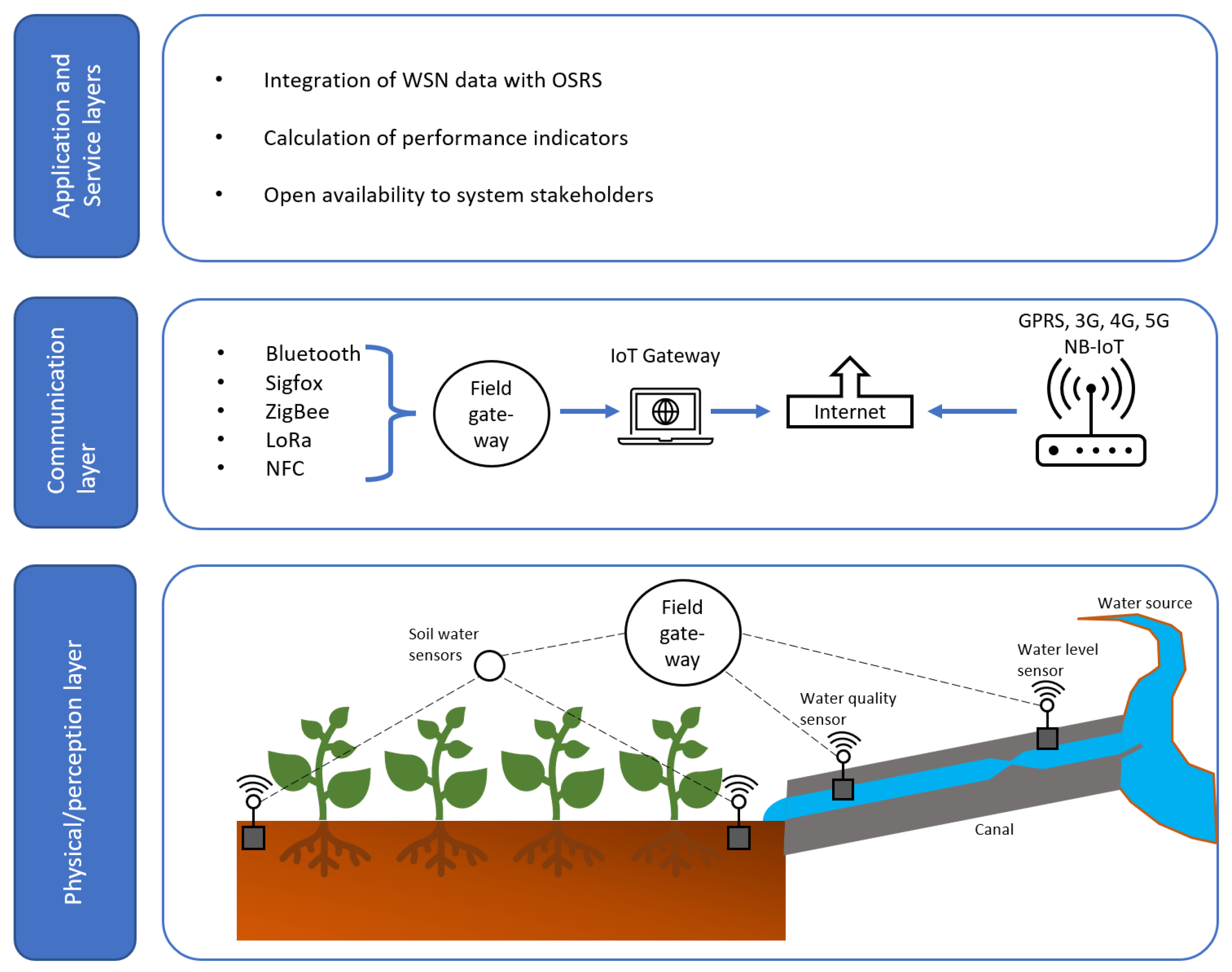
3.2. Networks with Connected Wireless Sensors

WSNs are capable of simultaneously sensing and transmitting a large volume of point observations of different variables. The use of solar panels and wireless connections allows for a distributed, relatively self-sufficient, and flexible network. An interesting implementation of WSNs in agriculture is for the automated management of irrigation systems, which has been an increasing area of study in recent years. A concise review by García et al. highlighted the cost limitations of these systems for precision agriculture installations [73]. Based on the mosaic of irrigation performance in Section 2.3, three irrigation monitoring variables to be sensed by WSNs are considered: water supply, soil moisture, and water quality. Two categories of WSNs for agricultural applications can be outlined: terrestrial wireless sensor networks (TWSN) and wireless underground sensor networks (WUSN) [74]. Each type has its advantages and disadvantages, TWSNs are more vulnerable to tampering or damage above the ground surface, while WUSNs require more effort and cost for installation and maintenance but are somewhat better protected below the surface, depending on the depth of installation and as long as other agricultural activities do not interfere with them. In the sections that follow, WSN refers mainly to TWSNs and reference to WUSNs is made explicitly.

Following the review carried out by Ojha et al., the WSN architecture in a use case for irrigation performance assessment would be a stationary, heterogeneous, and multi- or single-tier network [74]. The number of tiers depends on the size, layout, and organization of the irrigation scheme being monitored. This network architecture connects different types of sensors deployed in fixed locations. Water discharge sensors would be located at strategic points along the supply network, clusters of soil moisture sensors would be installed in farmers’ fields, and water quality sensors would be located at sampling locations in the supply and drainage points of fields and the wider irrigation network. This multi-tier system would in effect be a scaled up version of the single-tier system at farm level, to be used in installations monitoring several farms in tertiary and secondary irrigation scheme units.

Talavera et al. recommend a standard architecture for WSNs in agro-industrial applications [75]. In such an implementation, as shown in Figure 2, the architecture relies on a number of layers. In a precision agriculture installation, the physical layer includes perception and control layers. Figure 2 omits the control layer, as this article focuses on the monitoring of performance. The communication layer passes data to the services and applications, which present information derived from the data and provide security. The main focus of this section is on the physical and communication layers. The physical layer deals with perception to sample target variables and the communication layer transfers the data.

3.2.1. Supplied Water

The supplied water is a key variable at every scale of an irrigation scheme. Measuring discharge allows for supply information to be integrated over different temporal scales, with sampling points located at key locations in the scheme. The locations along the irrigation supply network mostly depend on the organizational nature of the irrigation scheme but typically will be at bifurcations or diversions. The type of infrastructure, either pipes or canals, will dictate which methods and sensors can be implemented.

For pipe flow, devices for measuring discharge need to be housed in the pipe itself. Some older mechanical devices such as propeller and paddlewheel meters require regular maintenance. More expensive electronic, magnetic, or ultrasonic devices require an energy source and proper calibration [76]. Unlike mechanical devices, the latter do not disrupt the flow in the pipe, reducing the risk of debris blockages. Venturi meters also benefit from a lack of obstruction and low maintenance requirements, although with some constriction of the pipe.

Measuring discharge in open canals typically requires water level sensors combined with knowledge of the canal cross-section or preferably a hydraulic structure such as a flume. The advantages of flumes include their accuracy, combined with low maintenance requirements, which offset the initial construction investment. Additional benefits are the relatively easy passage of debris and sediment, and that they allow visual inspection, encouraging transparency between stakeholders. Discharge is directly related to the water level at a specific point along the flume, meaning a stilling well can be used to ensure stable readings. Sensors of water level come in two categories: contact and non-contact. Contact sensors require installation in the water being measured and include pressure transducers, bubblers, shaft encoders, and acoustic sensors [77,78]. Non-contact sensors measure the level at a distance from the water surface and these may be radar, ultrasonic, or laser sensors. An example of a large-scale implementation of supply monitoring was given by Muhammad et al., where a stilling well equipped with a wireless ultrasonic range finding sensor was installed along irrigation canals to monitor water levels and estimate discharge with cross-section information [79].

3.2.2. Soil Water

In a review of IoT applications in agro-industry, it was found that 27.3% of monitoring applications focused on soil water content [75]. This number is likely to continue growing as more irrigation schemes adopt automated supply systems that monitor root zone depletion. In fact, soil water content is the most investigated parameter in the sector of irrigation monitoring through WSNs [73]. It is a critical component to be aware of for irrigation management, as recharging the root zone is the primary objective. However, due to its subterranean location, the low range of most sensors (especially if used in WUSN configurations), and three-dimensional spatial heterogeneity, this is not easily measured.

Underground sensors can be installed at interval depths to provide information about the vertical profile of soil water content. Specific operational requirements have to be considered, as signals are attenuated by the ground and a greater number of nodes are required to cover larger areas, as well as a higher energy consumption [74]. A variety of soil water sensors exist, with certain types better suited to specific soil texture, bulk density, salinity, and temperature levels [80]. Soil water sensors are generally separated into two groups: volumetric water content (VWC) sensors and water potential sensors.

VWC sensors measure a variable as a proxy of the fraction of the soil mixture that is water. These types of sensors include time domain reflectometry (TDR), frequency domain reflectometry (FDR), and capacitance [72,81]. TDR, FDR, and capacitance sensors rely on the fact that the dielectric constant of water is significantly greater than that of a typical soil. TDR probes measure the rate at which an electromagnetic pulse travels through the soil, which is related to the dielectric constant, with the pulse being slower in a wet soil than in a dry soil. TDR probes do not usually require calibration for a specific soil [81]. FDR relies on the frequency change of an electromagnetic pulse as it moves through the soil. FDR probes are cheaper than TDR probes and normally use less energy but are more prone to errors [82]. Capacitance probes measure the dielectric constant of the soil by measuring the time it takes for a capacitor that uses the soil as medium to charge [81]. FDR sensors are sometimes referred to as capacitance, as certain FDR sensor designs employ characteristics from both sensor types. Specific design aspects of TDR, FDR, and capacitance sensor types, such as operating frequency or number of frequency bands, make them more or less susceptible to soil salinity and other environmental conditions that affect accuracy. Aside from typical installation requirements to ensure good operation such as proper calibration, a crucial necessity is for the sensor to be installed in the soil without any air gaps.

Where VWC sensors measure a quantity of water in the soil, water potential sensors measure the energy content of that water. Water potential dictates the movement of water as it works toward equilibrium. The roots of crops must overcome the water potential to extract water from the soil, and if this energy requirement is too great, crops will begin wilting. The actual water content of the soil at the wilting point is dependent on specific soil characteristics and plant physiology. The most common sensor type for measuring water potential is the granular matrix electrical resistance sensor, which relies on the electrical resistance between two wire grids separated by a material that maintains the same water content as the surrounding soil [81]. As with FDR, TDR, and capacitance probes, proper contact with the soil with minimal air gaps is essential for accurate readings. Knowing the water potential alongside the VWC is key to irrigation scheduling. For the purpose of irrigation performance assessment, it informs about the usefulness of irrigation and whether the amount of water that has been added to the root zone can be used by the crop.

Knowledge of soil water content is key to evaluating the performance of irrigation schemes. Delivering water to the root zone of crops with proper timing and sufficient quantity is the prime objective of irrigation. In research by Jalilvand et al., changes in soil moisture from RS sources were used in the water balance as a means to estimate irrigation amounts [83]. Temporal patterns of irrigation could be detected to a certain extent. Studies in this direction are interesting, as we come close to closing the information gap between the micro and macro scales. However, caution is needed, as we do not know by what other processes the soil moisture may have been reduced, such as deep percolation or runoff [5]. There is also the potential to assimilate soil water data collected by WSN into forecasting models such as those discussed in Section 3.1.3, and the benefits to irrigation performance assessment need to be investigated.

3.2.3. Water Quality

The quality of supply and drainage water is a necessary monitoring input, not only when quantifying $E_E$, but also to ensure the basic requirements of the crop are being met. Irrigation water quality is defined by criteria that affect crop production, these are the total soluble salt content, relative proportion of sodium to calcium and magnesium ions, carbonate and bicarbonate content, pH, and other specific ions (chloride, sulfate, boron, and nitrate) [84,85]. Additionally, the presence of microbial pathogens must be monitored intermittently. For the purpose of an irrigation performance assessment framework, the main water quality criterion considered is total water salinity. This is to ensure that the basic requirement of irrigation water is met and the leaching requirement is satisfied. However, in the operation of an irrigation scheme, water sampling needs to take place at intervals, to monitor all of the water quality components.

Salinity affects the electrical conductivity (EC) of water, as higher amounts of total dissolved salts make the water more conductive. Soil water salinity is controlled by considering the leaching requirement, which is a necessary beneficial use of water in the field. $E_E$, as described in Section 2.2.2, factors in the salinity of irrigation water in assessing the performance of an irrigation scheme. Without the leaching requirement being met, the accumulation of salts in the soil would eventually make the soil unproductive. Monitoring the salinity of cultivated soils is important, to control land degradation. For this purpose, a number of methods are available, including assessing visual indicators, laboratory analysis of soil samples, in situ proximal sensors, and remote sensing methods. Proximal sensors measure the EC of the soil, while remote sensors rely on spectral signatures of soil salinity. Monitoring water quality relies on proximal sensors, whether in situ or in a laboratory. Measuring the EC with a sensor as part of a WSN allows for the calculation of total salt concentration [85]. A relatively low sampling rate is possible, with weekly to monthly measurements or potentially longer, depending on specific cases, as the salinity of irrigation water is unlikely to change over short periods if the source is unchanged.

3.2.4. Network Configuration

Sensors are located at nodes in a WSN and need to communicate with the Internet, to allow for ease of data collection and analysis. In applications of irrigation control alongside monitoring, sensor nodes communicate with actuator nodes that control water supply components such as pumps and valves. In this case, where solely monitoring is considered, the sensor nodes communicate with a gateway node that communicates with the Internet in a one-way direction. Due to the heterogeneous architecture of this WSN case, the nodes vary not only in sensing capability but also in transceiver ability [74]. Nodes are arranged in clusters that are related to the scale at which they monitor irrigation performance. An example WSN is illustrated in Figure 3, showing the hypothetical sector of an irrigation scheme containing two farms, each with three fields. Based on an architecture outlined by Ojha et al., the network is based on a cluster at field scale, which contains a discharge sensor, soil water sensor, and 3rd tier gateway nodes [74]. Each of the 3rd tier gateways communicates with the 2nd tier gateways at farm scale, which combined with a discharge sensor node at the point of farm supply constitute a farm scale cluster. The farm scale clusters then communicate with a 1st tier gateway node at sector level, which relays data to the remote sink communicating with the Internet.

Figure 3 describes the physical layer illustrated in Figure 2. Different protocols and communication systems are available for the communication layer. Communication from the sensor nodes to the gateways can be achieved using ZigBee, Bluetooth, NFC, WiFi, LoRA, or Sigfox [74,75]. Energy conservation has high priority when selecting the communications protocol, and this has to be balanced with the sampling frequency, power supply, communication distances, data packet size, and regularity of communication. The use of photovoltaic cells is common to recharge the batteries of sensors [73]. Alternative options for a WSN power supply are limited and the positioning of these cells must be critically assessed, as a growing crop may end up obscuring the power supply of a soil water sensor in a field. The final configuration of the WSN will depend on the specific requirement of the scheme, themselves hinging on its organizational structure and physical layout. Alongside costs, power considerations will have a major bearing on the overall design of the WSN.

3.3. Irrigation Monitoring and Irrigators

The increased integration of various sensors in agriculture is a major step towards “Smart Farming” or “Artificial Intelligence” in the agro-food sector [86]. In a review on big data in smart farming, Wolfert et al. laid out two extreme scenarios for the future of farming in a big data world, the first where farmers are one component of a highly integrated food supply chain made up of closed, proprietary systems, and the second with collaborative systems in which all stakeholders, including farmers, have flexibility in their business decisions [87].

Connecting sensors to the Internet, as part of the IoT, allows real-time monitoring of the soil water content in the root zone of irrigated crops. An important challenge remains the spatial variability in larger areas, such as large-scale irrigation schemes and wider catchments [88]. At farm level for high-value irrigated crops, this is often a practice existing as part of an automated high-tech field level irrigation system. However, to obtain representative values on a larger scheme, one needs to establish a large number of observation stations. In addition, the water reserve in the entire root zone is important at each location, and monitoring at least three depths is recommended. Recent developments in wireless sensors are described in [89].

Irrigation is not a phenomenon occurring in a test tube, to be studied from a distance and distilling recommendations to direct farmers. Rather, the data generated must be used meaningfully to inform and empower farmers, allowing them to make judgments on their own performance. Water users’ associations composed of farmers should be the meeting point where questions revolving around performance are resolved and actions are planned to correct low irrigation performance resulting from inequities. There is currently no single ideal model for irrigation performance assessment that can be applied to irrigation systems worldwide.

4. Discussion

As discussed in this article, irrigation performance has historically been defined in a variety of forms. A large number of indicators exist, and selecting or defining the most relevant must be carried out on a case-by-case basis. For this article, a limited, relevant selection was made, to layout a framework of the possible performance assessments and relevant technology currently available. While the stated objective of irrigation schemes is the replacement of root zone depletion and the efficient production of agricultural yields, this should not be achieved to the detriment of irrigation users. The wealth of data and sensors that can be employed to monitor and eventually automate the operations of an irrigation scheme should be deployed responsibly with respect to the complex hydro-social system that is an irrigation scheme. The main purpose of performance evaluation in irrigation is to maximize the perceived outputs from inputs to the system. However, this goal should only be pursued while empowering the more vulnerable users of an irrigation scheme.

This discussion section considers different time scales of assessment in the context of different groups. The spatial scales outlined in Section 2.3 are used here in conjunction with the three principal groups involved in the functioning of an irrigation scheme. The scales considered are the field/farm, the scheme, and the water resource. The groups are formed according to their main concern in the scheme. Group 1 is comprised of irrigators. These are users in direct contact with crop production and the end users of irrigation water. They operate at the field/farm and at the sub-sector scale in the scheme, as they often have contact with the irrigation supply network in proximity to their farm. Group 2 is concerned with the management of the irrigation scheme. This includes irrigation managers and engineers, as well as water user’s associations. Their influence is over the entire scheme, with the main focus being the irrigation supply network, its infrastructure, scheduling, and organization. Group 3 is involved with policy making and includes governmental actors such as environmental agencies and other regulatory bodies at the water resource scale, of which the irrigation scheme is one element. It is likely that an individual in an irrigation scheme is a member of more than one of the three groups. Farmers are often members of water management organizations, and they may also be politically active. The views of these groups and how they perceive irrigation performance is key to establishing a functional irrigation performance assessment approach. A summary of the discussion is visible in

Table 4. Summary of irrigation performance indicators at temporal and spatial scales and the influence of the three groups involved in an irrigation scheme.

		Spatial Scale
		Field/Farm	(Sub-)Sector/Scheme	Water Resource
Temporal Scale	Daily	$RIS$, $WDP$	$E_{APP}$	-
	Weekly to monthly	$RIS$, $WDP$	$E_C$, $E_{APP}$, $E_{CONV}$	$E_E$
	Seasonal	$RIS$, $WDP$, $WP$	$E_C$, $E_{APP}$, $E_{CONV}$	$E_E$

Irrigator. Irrigation manager. Policy maker.

, with consideration of spatial and temporal scales. The groups are attributed to the performance indicators over which they have influence.

4.1. Daily Assessment

At a daily time-step, performance assessment is mostly carried out for field and farm scale irrigation activities, with consideration of supply questions that impact these activities. For these activities and at this time scale, the main users concerned are group 1 and group 2, with the principal performance indicators $RIS$ and $WDP$ outlined in Equations (7) and (8), respectively. Assessing systems that involve plant processes such as $E_{APP}$ or $E_C$ is not feasible at a daily time scale. Filling the root zone reservoir of a crop may be completed in a single irrigation turn in less than a day, but this water is used through evapotranspiration over a longer time period. Moreover, reliable measurements of $E{T}_A$ based on OSRS are less available at a daily time-step, as outlined in Section 3.1.1.

For the daily calculation of $RIS$ and $WDP$, the measurement of supplied water by sensors, as described in Section 3.2.1, provides input data. The WSN must then be configured with a suitable sampling frequency to capture (sub-)daily variations in supply discharge, and the sampling points must be installed at relevant collection points along the supply network, as illustrated in Figure 3. Farmer-led organizations, at different scheme organizational levels, can identify strategic locations for this sampling to take place. With a sufficient number of sampling points in suitable locations, $E_{CONV}$ may also be calculated for particular sections of the supply network, as outlined in Equation (3). A requirement for this measurement is that the inputs and outputs of the assessed sections of the network are known.

Soil water sensors, as described in Section 3.2.2, allow $WDP$ to be estimated for individual fields. Relative changes in soil water content during an irrigation turn provides information on the effectiveness of delivery and application of the water. WSNs are most relevant to daily assessment, as typically there are no daily time-steps for OSRS-based measurements. Overall, close collaboration between group 1 and group 2 is necessary for daily irrigation performance assessment.

4.2. Weekly to Monthly Assessment

Weekly to monthly time-steps allow for the consideration of plant processes and the spatial and temporal up-scaling of the daily performance indicators mentioned in Section 4.1. Typically, irrigation planning on large irrigation schemes is implemented on a dekad or ten-day basis, fitting into this time scale. All three groups are involved at this time scale, with groups 1 and 2 having a similar influence as at the daily time-step, along with group 3 and their policy decisions potentially having a bearing on irrigation performance. This increase in time scale makes a comparison between different farms and sectors of an irrigation scheme possible. This is a strength of the irrigation performance indicators, which may highlight inequities or other issues in the scheme’s operation.

$E_{APP}$, and by association $E_C$, can be calculated as time periods of weeks to months, allowing the comparison of irrigation supply as described above with $E{T}_A$ from OSRS sources. $WDP$ and $RIS$, which at the daily scale could only be derived for individual farms, can now be calculated across the wider scheme as more irrigation turns are covered. The impact on group 1 is best explained with comparisons between irrigation users within the group. The relative performance of individual farms, sub-sectors, and sectors can be assessed. These comparisons then reflect on group 2, the internal functioning of the scheme, and its organizational structures.

The availability of $E{T}_A$ means $E_E$ from Equation (5) can also potentially be assessed, as data from water quality sensors described in Section 3.2.3 provide information on the LR. However, the requirement of measurement of the outflow from the irrigation scheme is complicated. Drainage networks for irrigation schemes are often less organized and structured than supply networks and therefore much more difficult to monitor. Where some kind of irrigation supply monitoring is already carried out in most irrigation schemes, outflow monitoring is less common. $E_E$ informs about the overall suitability of the irrigation scheme’s supply and is a measure of particular interest to group 3, as policy decisions should not only factor in the suitability of water for crop consumption but also the effect on users downstream of the irrigation scheme.

4.3. Seasonal Assessment

Looking at the seasonal time period, all groups and performance indicators are considered. $E_C$, along with $E_{APP}$ and $E_{CONV}$, $RIS$, $WDP$, and $E_E$ can all be integrated over the length of the growing season, with the possibility to highlight temporal dynamics in their variability. $WP$ can be calculated at this time scale, as the generation of seasonal biomass data from OSRS-based models is feasible. With sufficiently descriptive irrigation supply sampling locations and seasonal biomass production from the higher resolution OSRS options described in Section 3.1.2, it is possible to derive $WP$ information from field scale (depending on the field size) up to the wider scheme. This information can be further enriched by factoring in the economic value of crops.

Group 1 benefits from this information by comparing with their fellow irrigators how specific cropping choices have benefited them and the relative value of water in different areas of the scheme. Group 2 may choose to investigate certain areas of the scheme that are performing poorly when factoring in information from other performance indicators. These indicators provide a baseline against which any adjustment to irrigation distribution based on details gathered from investigations can be compared. Promises of increased efficiency and productivity from implementing high-technology irrigation systems, such as moving from surface irrigation to sprinkler or drip systems, can be verified. Group 3 gains insights into the economic dynamics of the irrigation scheme and can develop policies with greater knowledge, with the potential to verify the impacts of such policies.

5. Conclusions

Improving irrigation performance has been the aim of many projects in the past decades. The definitions surrounding irrigation performance have been argued over and complicate an already complex issue. The targets set out by these projects have often not been achieved, and the typical result has been more pressure on the water resource. This may be due to specific vested interests, private companies, state actors, etc. using marketing strategies to promote interest in irrigation projects. However, once the projects are complete, the actual benefits and drawbacks for individual farmers are difficult to quantify. Increased technification of irrigation does not necessarily lead to more efficient water use, but the higher quantity of sensors which tend to accompany these projects can be combined with the currently available OSRS data for the benefit of farmers.

The increasing accessibility and volume of remote sensing data and generally lowering costs of sensors have made more detailed irrigation performance assessment a possibility for many groups involved with irrigation. Ideally, an irrigation performance assessment project would be instigated and led by the actual irrigators and not only irrigation engineers and managers. The performance assessment should not be used to police the system but rather for farmers to inform themselves on issues and possible improvements and for scheme managers to address areas to allow better equity and quality of service. A significant level of expertise and financial input is required for the development of such a system. The installation and maintenance of a WSN involves both hardware and software requirements that are not commonplace, the use of OSRS data requires data processing capacity, and the combination of these tools needs dedicated online services. However, the potential opportunities are obvious, and a stepwise approach towards irrigation performance assessment is possible. The technology is available but is for the most part not leveraged by the direct end users of irrigation schemes.

The performance of an irrigation scheme is a complex issue. It cannot be solely reduced to simple ratios derived from a number of performance indicators. These indicators provide insight into potential areas of improvement for further investigation and, perhaps most importantly, can highlight possible issues of inequity in the hydro-social system that is an irrigation scheme. For example, should an irrigation user experiencing drawbacks related to their position in the scheme (e.g., less reliable access to water further from the head-end) receive some form of aid or assistance. These are the types of questions that may be approached as the complex interactions surrounding irrigation are elucidated.

References

1. Ertsen, M.W.; van der Spek, J. Modeling an irrigation ditch opens up the world. Hydrology and hydraulics of an ancient irrigation system in Peru. Phys. Chem. Earth Parts A/B/C 2009, 34, 176–191. [Google Scholar] [CrossRef]
2. FAO. The State of Food and Agriculture 2020. Overcoming Water Challenges in Agriculture; FAO: Rome, Italy, 2020. [Google Scholar] [CrossRef]
3. UN. World Population Projected to Reach 9.8 Billion in 2050, and 11.2 Billion in 2100 | UN DESA | United Nations Department of Economic and Social Affairs. Available online: https://www.un.org/development/desa/en/news/population/world-population-prospects-2017.html (accessed on 12 January 2021).
4. UN. Goal 6 | Department of Economic and Social Affairs. Available online: https://sdgs.un.org/goals/goal6 (accessed on 5 January 2021).
5. van Halsema, G.E.; Vincent, L. Efficiency and productivity terms for water management: A matter of contextual relativism versus general absolutism. Agric. Water Manag. 2012, 108, 9–15. [Google Scholar] [CrossRef]
6. Lankford, B. Fictions, fractions, factorials and fractures; on the framing of irrigation efficiency. Agric. Water Manag. 2012, 108, 27–38. [Google Scholar] [CrossRef]
7. Perry, C.J.; Steduto, P. Does Improved Irrigation Technology Save Water? A Review of the Evidence; FAO: Cairo, Egypt, 2017. [Google Scholar] [CrossRef]
8. Grafton, R.Q.; Williams, J.; Perry, C.J.; Molle, F.; Ringler, C.; Steduto, P.; Udall, B.; Wheeler, S.A.; Wang, Y.; Garrick, D.; et al. The paradox of irrigation efficiency. Science 2018, 361, 748–750. [Google Scholar] [CrossRef] [PubMed]
9. Boelens, R.; Vos, J. The danger of naturalizing water policy concepts: Water productivity and efficiency discourses from field irrigation to virtual water trade. Agric. Water Manag. 2012, 108, 16–26. [Google Scholar] [CrossRef]
10. Lowder, S.K.; Skoet, J.; Raney, T. The Number, Size, and Distribution of Farms, Smallholder Farms, and Family Farms Worldwide. World Dev. 2016, 87, 16–29. [Google Scholar] [CrossRef]
11. D’Odorico, P.; Rulli, M.C.; Dell’Angelo, J.; Davis, K.F. New frontiers of land and water commodification: Socio-environmental controversies of large-scale land acquisitions. Land Degrad. Dev. 2017, 28, 2234–2244. [Google Scholar] [CrossRef]
12. Seckler, D. The New Era of Water Resources Management: From “Dry” to “Wet” Water Savings; Vol. Research Report 1; OCLC: 643562595; International Water Management Institute: Colombo, Sri Lanka, 1996. [Google Scholar]
13. Willardson, L.S.; Allen, R.G.; Frederiksen, H.D. Elimination of Irrigation Efficiencies. In Proceedings of the Question 47 Irrigation Planning and Management Measures in Harmony with the Environment, Denver, Colorado, USA, 19–22 October 1994; p. 17. [Google Scholar]
14. Israelsen, O.W.; Criddle, W.D.; Fuhriman, D.K.; Hansen, V.E. Bulletin No. 311—Water-Application Efficiencies in Irrigation. UAES Bull. 1944, 273. [Google Scholar]
15. Keller, A.A.; Keller, J. Effective Efficiency: A Water Use Efficiency Concept for Allocating Freshwater Resources; Discussion Paper 22; Center for Economic Policy Studies, Winrock International: Arlington, VA, USA, 1995. [Google Scholar]
16. Giordano, M.; Turral, H.; Scheierling, S.M.; Treguer, D.O.; McCornick, P.G. Beyond “More Crop per Drop”: Evolving Thinking on Agricultural Water Productivity; Technical Report; International Water Management Institute (IWMI): Colombo, Sri Lanka; The World Bank: Washington, DC, USA, 2017. [Google Scholar] [CrossRef]
17. Lankford, B.; Closas, A.; Dalton, J.; López Gunn, E.; Hess, T.; Knox, J.W.; van der Kooij, S.; Lautze, J.; Molden, D.; Orr, S.; et al. A scale-based framework to understand the promises, pitfalls and paradoxes of irrigation efficiency to meet major water challenges. Glob. Environ. Chang. 2020, 65, 102182. [Google Scholar] [CrossRef]
18. Koech, R.; Langat, P. Improving Irrigation Water Use Efficiency: A Review of Advances, Challenges and Opportunities in the Australian Context. Water 2018, 10, 1771. [Google Scholar] [CrossRef]
19. Allen, R.G.; Pereira, L.S.; Raes, D.; Smith, M. (Eds.) Crop Evapotranspiration: Guidelines for Computing Crop Water Requirements; Number 56 in FAO Irrigation and Drainage Paper; Food and Agriculture Organization of the United Nations: Rome, Italy, 1998. [Google Scholar]
20. Jensen, M.E. Beyond irrigation efficiency. Irrig. Sci. 2007, 25, 233–245. [Google Scholar] [CrossRef]
21. Parra, L.; Botella-Campos, M.; Puerto, H.; Roig-Merino, B.; Lloret, J. Evaluating Irrigation Efficiency with Performance Indicators: A Case Study of Citrus in the East of Spain. Agronomy 2020, 10, 1359. [Google Scholar] [CrossRef]
22. Bos, M.G. Performance indicators for irrigation and drainage. Irrig. Drain. Syst. 1997, 11, 119–137. [Google Scholar] [CrossRef]
23. Zafar, A.; Prathapar, S.; Bastiaanssen, W.; Awan, W.K.; Cai, X.; Manunta, P. Optimization of Canal Management Using Satellite Measurements; Series: ADB Briefs; Asian Development Bank: Manila, Philippines, 2021; ISBN 9789292627027/9789292627010. [Google Scholar] [CrossRef]
24. Massari, C.; Modanesi, S.; Dari, J.; Gruber, A. A Review of Irrigation Information Retrievals from Space and Their Utility for Users. Remote Sens. 2021, 13, 4112. [Google Scholar] [CrossRef]
25. Vanino, S.; Nino, P.; De Michele, C.; Falanga Bolognesi, S.; D’Urso, G.; Di Bene, C.; Pennelli, B.; Vuolo, F.; Farina, R.; Pulighe, G.; et al. Capability of Sentinel-2 data for estimating maximum evapotranspiration and irrigation requirements for tomato crop in Central Italy. Remote Sens. Environ. 2018, 215, 452–470. [Google Scholar] [CrossRef]
26. Segarra, J.; Buchaillot, M.L.; Araus, J.L.; Kefauver, S.C. Remote Sensing for Precision Agriculture: Sentinel-2 Improved Features and Applications. Agronomy 2020, 10, 641. [Google Scholar] [CrossRef]
27. Wulder, M.A.; Roy, D.P.; Radeloff, V.C.; Loveland, T.R.; Anderson, M.C.; Johnson, D.M.; Healey, S.; Zhu, Z.; Scambos, T.A.; Pahlevan, N.; et al. Fifty years of Landsat science and impacts. Remote Sens. Environ. 2022, 280, 113195. [Google Scholar] [CrossRef]
28. Phiri, D.; Simwanda, M.; Salekin, S.; Nyirenda, V.; Murayama, Y.; Ranagalage, M. Sentinel-2 Data for Land Cover/Use Mapping: A Review. Remote Sens. 2020, 12, 2291. [Google Scholar] [CrossRef]
29. Zhang, K.; Kimball, J.S.; Running, S.W. A review of remote sensing based actual evapotranspiration estimation. WIREs Water 2016, 3, 834–853. [Google Scholar] [CrossRef]
30. Chao, Z.; Liu, N.; Zhang, P.; Ying, T.; Song, K. Estimation methods developing with remote sensing information for energy crop biomass: A comparative review. Biomass Bioenergy 2019, 122, 414–425. [Google Scholar] [CrossRef]
31. Swinnen, E.; Van Hoolst, R. Algorithm Theoretical Basis Document Dry Matter Productivity (DMP) Gross Dry Matter Productivity (GDMP) Collection 300 m, Version 1, Issue I1.12. Copernicus Global Land Operation ‘Vegetation and Energy’. 2019. Available online: https://land.copernicus.eu/en/technical-library/algorithm-theoretical-basis-document-dry-and-gross-dry-matter-productivity-version-1/@@download/file (accessed on 13 June 2024).
32. FAO. WaPOR Database Methodology, 2nd ed.; FAO: Rome, Italy, 2020. [Google Scholar] [CrossRef]
33. ELeaf; VITO; ITC; WaterWatch; University of Twente. WaPOR Data Manual Evapotranspiration; FAO: Rome, Italy, 2020; Volume 2.2. [Google Scholar]
34. Sun, Z.; Wang, X.; Zhang, X.; Tani, H.; Guo, E.; Yin, S.; Zhang, T. Evaluating and comparing remote sensing terrestrial GPP models for their response to climate variability and CO2 trends. Sci. Total Environ. 2019, 668, 696–713. [Google Scholar] [CrossRef]
35. Pan, S.; Pan, N.; Tian, H.; Friedlingstein, P.; Sitch, S.; Shi, H.; Arora, V.K.; Haverd, V.; Jain, A.K.; Kato, E.; et al. Evaluation of global terrestrial evapotranspiration using state-of-the-art approaches in remote sensing, machine learning and land surface modeling. Hydrol. Earth Syst. Sci. 2020, 24, 1485–1509. [Google Scholar] [CrossRef]
36. Bastiaanssen, W.G.M.; Menenti, M.; Feddes, R.A.; Holtslag, A.A.M. A remote sensing surface energy balance algorithm for land (SEBAL). 1. Formulation. J. Hydrol. 1998, 212–213, 198–212. [Google Scholar] [CrossRef]
37. Laipelt, L.; Henrique Bloedow Kayser, R.; Santos Fleischmann, A.; Ruhoff, A.; Bastiaanssen, W.; Erickson, T.A.; Melton, F. Long-term monitoring of evapotranspiration using the SEBAL algorithm and Google Earth Engine cloud computing. ISPRS J. Photogramm. Remote. Sens. 2021, 178, 81–96. [Google Scholar] [CrossRef]
38. Allen, R.G.; Tasumi, M.; Trezza, R. Satellite-Based Energy Balance for Mapping Evapotranspiration with Internalized Calibration (METRIC)—Model. J. Irrig. Drain. Eng. 2007, 133, 380–394. [Google Scholar] [CrossRef]
39. Hong, S.; Hendrickx, J.M.; Allen, R.G. Comparison of Remote Sensing Energy Balance Models: Sebal V.S. Metric. In Proceedings of the AGU Fall Meeting Abstracts ADS Bibcode: 2008AGUFM.H43G1094H, San Francisco, CA, USA, 15–19 December 2008; American Geophysical Union: Washington, DC, USA, 2008. [Google Scholar]
40. Jaafar, H.H.; Ahmad, F.A. Time series trends of Landsat-based ET using automated calibration in METRIC and SEBAL: The Bekaa Valley, Lebanon. Remote Sens. Environ. 2020, 238, 111034. [Google Scholar] [CrossRef]
41. Kilic, A.; Allen, R.G.; Blankenau, P.; Revelle, P.; Ozturk, D.; Huntington, J. Global production and free access to Landsat-scale Evapotranspiration with EEFlux and eeMETRIC. In Proceedings of the 6th Decennial National Irrigation Symposium, San Diego, CA, USA, 6–8 December 2021; American Society of Agricultural and Biological Engineers: St. Joseph, MI, USA, 2021. [Google Scholar] [CrossRef]
42. Norman, J.; Kustas, W.; Humes, K. Source approach for estimating soil and vegetation energy fluxes in observations of directional radiometric surface temperature. Agric. For. Meteorol. 1995, 77, 263–293. [Google Scholar] [CrossRef]
43. French, A.N.; Hunsaker, D.J.; Thorp, K.R. Remote sensing of evapotranspiration over cotton using the TSEB and METRIC energy balance models. Remote Sens. Environ. 2015, 158, 281–294. [Google Scholar] [CrossRef]
44. Anderson, M.C.; Norman, J.M.; Mecikalski, J.R.; Otkin, J.A.; Kustas, W.P. A climatological study of evapotranspiration and moisture stress across the continental United States based on thermal remote sensing: 1. Model formulation. J. Geophys. Res. 2007, 112, D10117. [Google Scholar] [CrossRef]
45. Norman, J.M.; Anderson, M.C.; Kustas, W.P.; French, A.N.; Mecikalski, J.; Torn, R.; Diak, G.R.; Schmugge, T.J.; Tanner, B.C.W. Remote sensing of surface energy fluxes at 101-m pixel resolutions: Remote sensing of surface energy fluxes. Water Resour. Res. 2003, 39, 1221. [Google Scholar] [CrossRef]
46. Fisher, J.B.; Lee, B.; Purdy, A.J.; Halverson, G.H.; Dohlen, M.B.; Cawse-Nicholson, K.; Wang, A.; Anderson, R.G.; Aragon, B.; Arain, M.A.; et al. ECOSTRESS: NASA’s Next Generation Mission to Measure Evapotranspiration From the International Space Station. Water Resour. Res. 2020, 56, e2019WR026058. [Google Scholar] [CrossRef]
47. Anderson, M.C. Interoperability of ECOSTRESS and Landsat for mapping evapotranspiration time series at sub-field scales. Remote Sens. Environ. 2021, 252, 112189. [Google Scholar] [CrossRef]
48. Running, S.W.; Mu, Q.; Zhao, M.; Moreno, A. User’s Guide MODIS Global Terrestrial Evapotranspiration (ET) Product NASA Earth Observing System MODIS Land Algorithm (For Collection 6.1). Version 1.1. MODIS Land Team. 2021. Available online: https://www.ntsg.umt.edu/project/modis/user-guides/mod16c61usersguidev11mar112021.pdf (accessed on 13 June 2024).
49. Pelgrum, H.; Miltenburg, I.J.; Cheema, M.J.M.; Klaasse, A. ETLook: A novel continental evapotranspiration algorithm. In Proceedings of the Remote Sensing and Hydrology, Jackson Hole, WY, USA, 27–30 September 2010. [Google Scholar]
50. Bastiaanssen, W.G.M.; Cheema, M.J.M.; Immerzeel, W.W.; Miltenburg, I.J.; Pelgrum, H. Surface energy balance and actual evapotranspiration of the transboundary Indus Basin estimated from satellite measurements and the ETLook model: Energy balance and et of the indus basin. Water Resour. Res. 2012, 48, W11512. [Google Scholar] [CrossRef]
51. FAO WaPOR. 2021. Available online: https://wapor.apps.fao.org/home/WAPOR_2/1 (accessed on 22 June 2021).
52. Priestley, C.H.B.; Taylor, R.J. On the Assessment of Surface Heat Flux and Evaporation Using Large-Scale Parameters. Mon. Weather Rev. 1972, 100, 81–92. [Google Scholar] [CrossRef]
53. Fisher, J.B. Level-3 Evapotranspiration L3(ET_PT-JPL) Algorithm Theoretical Basis Document; NASA: Pasadena, CA, USA, 2018. [Google Scholar]
54. Guzinski, R.; Nieto, H.; Sandholt, I.; Karamitilios, G. Modelling High-Resolution Actual Evapotranspiration through Sentinel-2 and Sentinel-3 Data Fusion. Remote Sens. 2020, 12, 1433. [Google Scholar] [CrossRef]
55. DHI GRAS; IRTA; Sandholt. User Manual for Sen-ET Plugin; V1.1.0; ESA: Paris, France, 2020; Available online: https://www.esa-sen4et.org/static/media/sen-et-user-manual-v1.1.0.5d1ac526.pdf (accessed on 12 June 2024).
56. Martens, B.; Miralles, D.G.; Lievens, H.; van der Schalie, R.; de Jeu, R.A.M.; Fernández-Prieto, D.; Beck, H.E.; Dorigo, W.A.; Verhoest, N.E.C. GLEAM v3: Satellite-based land evaporation and root-zone soil moisture. Geosci. Model Dev. 2017, 10, 1903–1925. [Google Scholar] [CrossRef]
57. GLEAM Global Land Evaporation Amsterdam Model. 2023. Available online: https://www.gleam.eu/ (accessed on 19 January 2023).
58. Tang, R.; Li, Z.L.; Tang, B. An application of the Ts–VI triangle method with enhanced edges determination for evapotranspiration estimation from MODIS data in arid and semi-arid regions: Implementation and validation. Remote Sens. Environ. 2010, 114, 540–551. [Google Scholar] [CrossRef]
59. Nugraha, A.S.A.; Kamal, M.; Murti, S.H.; Widyatmanti, W. Development of the triangle method for drought studies based on remote sensing images: A review. Remote Sens. Appl. Soc. Environ. 2023, 29, 100920. [Google Scholar] [CrossRef]
60. OpenET Filling the Biggest Gap in Water Management. 2023. Available online: https://openetdata.org/ (accessed on 19 January 2023).
61. Lagouarde, J.P.; Bhattacharya, B.; Crébassol, P.; Gamet, P.; Babu, S.S.; Boulet, G.; Briottet, X.; Buddhiraju, K.; Cherchali, S.; Dadou, I.; et al. The Indian-French Trishna Mission: Earth Observation in the Thermal Infrared with High Spatio-Temporal Resolution. In Proceedings of the IGARSS 2018–2018 IEEE International Geoscience and Remote Sensing Symposium, Valencia, Spain, 22–27 July 2018; pp. 4078–4081. [Google Scholar] [CrossRef]
62. Koetz, B.; Bastiaanssen, W.; Berger, M.; Defourney, P.; Del Bello, U.; Drusch, M.; Drinkwater, M.; Duca, R.; Fernandez, V.; Ghent, D.; et al. High Spatio- Temporal Resolution Land Surface Temperature Mission—A Copernicus Candidate Mission in Support of Agricultural Monitoring. In Proceedings of the IGARSS 2018 IEEE International Geoscience and Remote Sensing Symposium, Valencia, Spain, 22–27 July 2018; pp. 8160–8162. [Google Scholar] [CrossRef]
63. Airbus. The Copernicus LSTM Expansion mission moves a step closer to helping climate change adaptation. Airbus. 7 November 2022. Available online: https://www.airbus.com/en/newsroom/stories/2022-11-the-copernicus-lstm-expansion-mission-moves-a-step-closer-to-helping (accessed on 24 January 2023).
64. Smets, B.; Swinnen, E.; Van Hoolst, R. Product User Manual Dry Matter Productivity (DMP) Gross Dry Matter Productivity (GDMP), Version 1, Issue I1.22. Copernicus Global Land Operations ‘Vegetation and Energy’. 2019. Available online: https://land.copernicus.eu/en/technical-library/product-user-manual-dry-and-gross-dry-matter-productivity-version-1/@@download/file (accessed on 12 June 2024).
65. Li, X.; Xiao, J.; Fisher, J.B.; Baldocchi, D.D. ECOSTRESS estimates gross primary production with fine spatial resolution for different times of day from the International Space Station. Remote Sens. Environ. 2021, 258, 112360. [Google Scholar] [CrossRef]
66. Deb, P.; Abbaszadeh, P.; Moradkhani, H. An ensemble data assimilation approach to improve farm-scale actual evapotranspiration estimation. Agric. For. Meteorol. 2022, 321, 108982. [Google Scholar] [CrossRef]
67. Luo, L.; Sun, S.; Xue, J.; Gao, Z.; Zhao, J.; Yin, Y.; Gao, F.; Luan, X. Crop yield estimation based on assimilation of crop models and remote sensing data: A systematic evaluation. Agric. Syst. 2023, 210, 103711. [Google Scholar] [CrossRef]
68. Jin, X.; Kumar, L.; Li, Z.; Feng, H.; Xu, X.; Yang, G.; Wang, J. A review of data assimilation of remote sensing and crop models. Eur. J. Agron. 2018, 92, 141–152. [Google Scholar] [CrossRef]
69. Yuan, Q.; Shen, H.; Li, T.; Li, Z.; Li, S.; Jiang, Y.; Xu, H.; Tan, W.; Yang, Q.; Wang, J.; et al. Deep learning in environmental remote sensing: Achievements and challenges. Remote Sens. Environ. 2020, 241, 111716. [Google Scholar] [CrossRef]
70. Chia, M.Y.; Huang, Y.F.; Koo, C.H.; Fung, K.F. Recent Advances in Evapotranspiration Estimation Using Artificial Intelligence Approaches with a Focus on Hybridization Techniques—A Review. Agronomy 2020, 10, 101. [Google Scholar] [CrossRef]
71. Bahrami, H.; Homayouni, S.; Safari, A.; Mirzaei, S.; Mahdianpari, M.; Reisi-Gahrouei, O. Deep Learning-Based Estimation of Crop Biophysical Parameters Using Multi-Source and Multi-Temporal Remote Sensing Observations. Agronomy 2021, 11, 1363. [Google Scholar] [CrossRef]
72. Abioye, E.A.; Abidin, M.S.Z.; Mahmud, M.S.A.; Buyamin, S.; Ishak, M.H.I.; Rahman, M.K.I.A.; Otuoze, A.O.; Onotu, P.; Ramli, M.S.A. A review on monitoring and advanced control strategies for precision irrigation. Comput. Electron. Agric. 2020, 173, 105441. [Google Scholar] [CrossRef]
73. García, L.; Parra, L.; Jimenez, J.M.; Lloret, J.; Lorenz, P. IoT-Based Smart Irrigation Systems: An Overview on the Recent Trends on Sensors and IoT Systems for Irrigation in Precision Agriculture. Sensors 2020, 20, 1042. [Google Scholar] [CrossRef]
74. Ojha, T.; Misra, S.; Raghuwanshi, N.S. Wireless sensor networks for agriculture: The state-of-the-art in practice and future challenges. Comput. Electron. Agric. 2015, 118, 66–84. [Google Scholar] [CrossRef]
75. Talavera, J.M.; Tobón, L.E.; Gómez, J.A.; Culman, M.A.; Aranda, J.M.; Parra, D.T.; Quiroz, L.A.; Hoyos, A.; Garreta, L.E. Review of IoT applications in agro-industrial and environmental fields. Comput. Electron. Agric. 2017, 142, 283–297. [Google Scholar] [CrossRef]
76. Boman, B.; Shukla, S. Water Measurement for Agricultural Irrigation and Drainage Systems: Circular 1495/CH153, 10/2006. EDIS 2006, 2006, 1–12. [Google Scholar] [CrossRef]
77. YSI. Water Level Measurement, Sensors, Monitoring Applications; YSI: Yellow Springs, OH, USA, 2023; Available online: https://www.ysi.com/parameters/level (accessed on 24 February 2023).
78. RSHydro. Open Channel Flow Meters & Flow Measurement Specialists; RSHydro: Bromsgrove, UK, 2023; Available online: https://www.rshydro.co.uk/flow-meters/open-channel-flowmeter/ (accessed on 24 February 2023).
79. Muhammad, A.; Haider, B.; Ahmad, Z. IoT Enabled Analysis of Irrigation Rosters in the Indus Basin Irrigation System. Procedia Eng. 2016, 154, 229–235. [Google Scholar] [CrossRef]
80. Mittelbach, H.; Lehner, I.; Seneviratne, S.I. Comparison of four soil moisture sensor types under field conditions in Switzerland. J. Hydrol. 2012, 430–431, 39–49. [Google Scholar] [CrossRef]
81. Sharma, V. Soil Moisture Sensors for Irrigation Scheduling; University of Minnesota Extension: St Paul, MN, USA, 2019; Available online: https://extension.umn.edu/irrigation/soil-moisture-sensors-irrigation-scheduling (accessed on 19 April 2023).
82. Hardie, M. Review of Novel and Emerging Proximal Soil Moisture Sensors for Use in Agriculture. Sensors 2020, 20, 6934. [Google Scholar] [CrossRef] [PubMed]
83. Jalilvand, E.; Tajrishy, M.; Ghazi Zadeh Hashemi, S.A.; Brocca, L. Quantification of irrigation water using remote sensing of soil moisture in a semi-arid region. Remote Sens. Environ. 2019, 231, 111226. [Google Scholar] [CrossRef]
84. Bauder, T.A.; Waskom, R.M.; Sutherland, P.L.; Davis, J.G. Irrigation Water Quality Criteria; Fact Sheet No. 0.506; Colorado State University: Fort Collins, CO, USA, 2014. [Google Scholar]
85. Zaman, M.; Shahid, S.A.; Heng, L. Guideline for Salinity Assessment, Mitigation and Adaptation Using Nuclear and Related Techniques; Springer: Cham, Switzerland, 2018. [Google Scholar] [CrossRef]
86. De Baerdemaeker, J. Artificial Intelligence in the Agri-Food Sector: Applications, Risks and Impacts; OCLC: 1376263180; European Parliament: Brussels, Belgium, 2023. [Google Scholar]
87. Wolfert, S.; Ge, L.; Verdouw, C.; Bogaardt, M.J. Big Data in Smart Farming—A review. Agric. Syst. 2017, 153, 69–80. [Google Scholar] [CrossRef]
88. Bogena, H.; Herbst, M.; Huisman, J.; Rosenbaum, U.; Weuthen, A.; Vereecken, H. Potential of Wireless Sensor Networks for Measuring Soil Water Content Variability. Vadose Zone J. 2010, 9, 1002–1013. [Google Scholar] [CrossRef]
89. Bogena, H.R.; Weuthen, A.; Huisman, J.A. Recent Developments in Wireless Soil Moisture Sensing to Support Scientific Research and Agricultural Management. Sensors 2022, 22, 9792. [Google Scholar] [CrossRef]
Figure 1. Model for irrigation performance assessment across scales based on the BAIE model at field level and on the SLIE model at scheme and catchment levels. Water supply (W), crop transpiration (T), soil evaporation (E), return flow (R), and deep percolation (D) describe water flows across three spatial scales: field, scheme, and catchment. The fraction category of each flow is indicated by the subscript: beneficial consumption (BC), non-beneficial consumption (NBC), recoverable fraction (RF), and non-recoverable fraction (NRF). The scale is indicated by the superscript.
Water 16 01762 g001
Figure 2. WSN irrigation performance monitoring architecture based on [75].
Water 16 01762 g002
Figure 3. Architecture of a WSN for monitoring irrigation performance from field scale up to irrigation scheme sector scale. This layout or specific parts of it can be replicated at various scales throughout a large irrigation scheme with many stakeholders.
Water 16 01762 g003