Risk Assessment and Control for Geohazards at Multiple Scales: An Insight from the West Han River of Gansu Province in China

Abstract

Risk assessment provides a powerful tool for the early warning and risk mitigation of geohazards. However, few efforts have been made regarding risk assessment and dynamic control at multiple scales. With respect to this issue, the West Han River catchment in the Gansu Province of China was taken as a study area, and geohazard risk assessments at three different scales were carried out, namely regional, local and site scales. Hazard assessment was performed using the combination of the information value and hierarchical analysis models, infinite slope stability model, and FLO-2D model. Vulnerability was estimated from two viewpoints, including physical vulnerability and social vulnerability, by applying remote sensing and semi-quantitative methods. Finally, risk mapping and zonation was obtained from the products of hazard and vulnerability, and corresponding measures of risk management and control at different scales were recommended. The results indicated that the geohazard risk at the regional scale was the highest under the earthquake and rainfall conditions with a 100-year (100a) return period, respectively, and the area of very high risk level reached 5%. When the rainfall condition had a return period of 50 years, only 1% of the area was located in the very high-risk region. Additionally, the overall risk was higher in the central and northeastern parts of the region under heavy rainfall and earthquake conditions. The overall risk level in Longlin-Leiba Town (at the local scale) responded more significantly to heavy rainfall conditions, with higher risk in the southwestern, central, and northeastern parts of the region. For the site scale (Wujiagou debris flow), only 2% of the total area was identified as very high-risk even under heavy rainfall with a 100a return period, but the proportions for the low and moderate levels reached 30% and 56%, respectively. The present study can provide scientific references for geohazard risk assessment and control.

1. Introduction

Geological hazards are one of the most destructive natural hazard phenomena worldwide [1,2], often causing great harm to the lives and survival of local inhabitants and seriously damaging infrastructure development. Geohazard risk assessment has been an effective tool for geohazard prevention and control among government departments [3,4], and its results can show the probability of a geohazard’s occurrence and its scale [5], so exploring geohazard risk assessment at different scales is always an important topic for the scientific community.

Geohazard risk assessment mainly includes two steps: hazard assessment and vulnerability assessment. Among them, hazard assessment includes both qualitative and quantitative methods [6], and the qualitative methods mainly use historical landslide inventory data to obtain hazard zoning maps for specific scenarios or rely on the experience of experts with rich expertise in hazard mapping [7], so they are also called “knowledge-driven models”. However, these models are generally more subjective, and their accuracy needs to be improved. In contrast, quantitative models [8,9,10] are often based on a specific theoretical or numerical method to obtain quantitative hazard assessment results, and therefore, the results are more reliable. Deterministic models are an important branch of this class of methods that can calculate slope stability based on the physical properties of the controlling geomorphic processes, thus better reflecting the landslide instability damage process. The main deterministic models that have been developed [11,12] include SHALSTAB [13], SCOOPS3D [14], TRIGRS [15], SLIP [16], FSLAM [17], etc. Additionally, some studies have superimposed the temporal probability of geohazard triggering factors (generally rainfall or seismic conditions) on the basis of susceptibility assessment to obtain hazard assessment results quantitatively. The methods used for susceptibility assessment mainly include four categories, namely expert empirical models [18], physics-based models [19], statistical models [20,21], and machine learning (ML) models [22,23,24]. Several comparative studies [25,26] have shown that statistical and ML models typically have higher precision and accuracy and, thus, have been widely used for tasks in landslide susceptibility assessment, such as artificial neural networks (ANNs) and random forest (RF).

Vulnerability is a key component of geohazard risk assessment. Due to its complex nature, many different concepts and methods exist in the literature to assess vulnerability [27,28]. In general, susceptibility is an inherent characteristic of the element at risk, i.e., the nature of being affected or vulnerable to damage due to an impact hazard of a specific intensity [29,30]. There are three main methods currently used for vulnerability assessment, as follows: (i) a vulnerability analysis based on the opinions of experts [31] whose analytical data are obtained by collecting the opinions of a large number of experts on the assessment of regions in different damage states, but these assessment results rely on the subjective judgment of experts and are less accurate; (ii) an empirical analysis based on field surveys [32] whose data are usually derived from historical disaster survey data in the same region; (iii) a theoretical analysis based on a numerical simulation [33,34], whose analytical data are directly derived from the results of theoretical numerical simulations, and the analytical data used are more controllable; therefore, theoretical analyses have become one of the most widely used vulnerability analysis methods. The vulnerability curves or functions required for this method can be obtained in various ways, the earliest being an elastic response spectrum analysis [35] and the CSM method [36]. With the improvement in computer computing efficiency, the most popular computational method is nonlinear time course analysis (NLTHA).

Regarding risk assessment, previous studies have mostly focused on three aspects, namely the regional scale [37,38], local scale [39] and site scale [40]. Generally, the local scale and regional scale have usually been defined as 1:25,000–1:5000 and 1:250,000–1:25,000, respectively [41], and the site scale is the largest (>1:5000). Hence, the specific methods for the modeling and analysis of these scales often have some differences. However, fewer comparative studies have been conducted from multiple scales in a region at the same time, such as Dalia Bach Kriechbaum (2009), who conducted a risk assessment of landslide hazards at two scales through bivariate modeling techniques and multivariate statistical methods. Nonetheless, overall, the number of such studies is still low, and there is an urgent need to increase the number of relevant case studies in multiple regions around the world [42,43,44].

To address these issues, this study selected the West Han River watershed in the Gansu region of China as the study area and carried out geohazard risk assessment at three different scales. Finally, corresponding risk management recommendations based on the risk results were proposed, aimed at providing assistance in exploring theoretical and technical issues in multi-scale geohazard risk assessment.

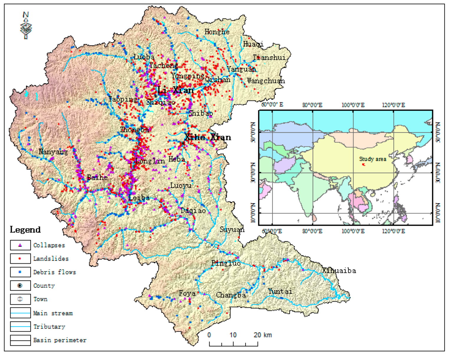
2. Study Area and Data Preparation

2.1. Risk Results and Assessment at Regional Scale

The investigation area of this study includes three different scales, i.e., the regional scale, local scale, and site scale. Among them, the regional scale is the Longnan West Han River watershed, the town scale is the key area of the Longlin-Leiba Town section, and the site scale is the Wujiagou debris-flow landslide.

The West Han River watershed is located in the mountainous area of Longnan; it belongs to the southwest of the Loess Plateau, and the northeast of the Qinghai-Tibet Plateau is adjacent. It has a basin area of 10,178 km², the overall topography of the northwest high is, while the southeast is low. With a territory of overlapping mountains, steep slopes, and deep valleys, gullies, and complex terrain, the region’s landscape is divided into loess hills, low mountains, low and medium mountains, medium mountains, high and medium mountains, a river valley plains area, and six other categories. The stratigraphy of the area ranges from the Silurian of the Late Paleozoic to the Quaternary of the Cenozoic, and the lithology is mainly slate, sandstone, and tuff. The study area has a temperate continental monsoon climate with abundant rainfall and significant horizontal and vertical changes in climate, with an average annual rainfall of 551.4 mm. Water resources are abundant, and the river network is dense, plume-like, and dendritic. The watershed mainly involves four administrative districts, namely Lixian, Xihe, Chengxian, and Kangxian, with a total resident population of about 1.2 million. In recent years, the scope of human engineering activities in the region has been expanding, mainly in infrastructure construction, especially road construction, steep slope cultivation, and the development of mineral resources. At the same time, due to the low surface vegetation coverage caused due to previous deforestation, the geological disasters in the area are very serious and pose a great threat to people’s lives and the safety of their property.

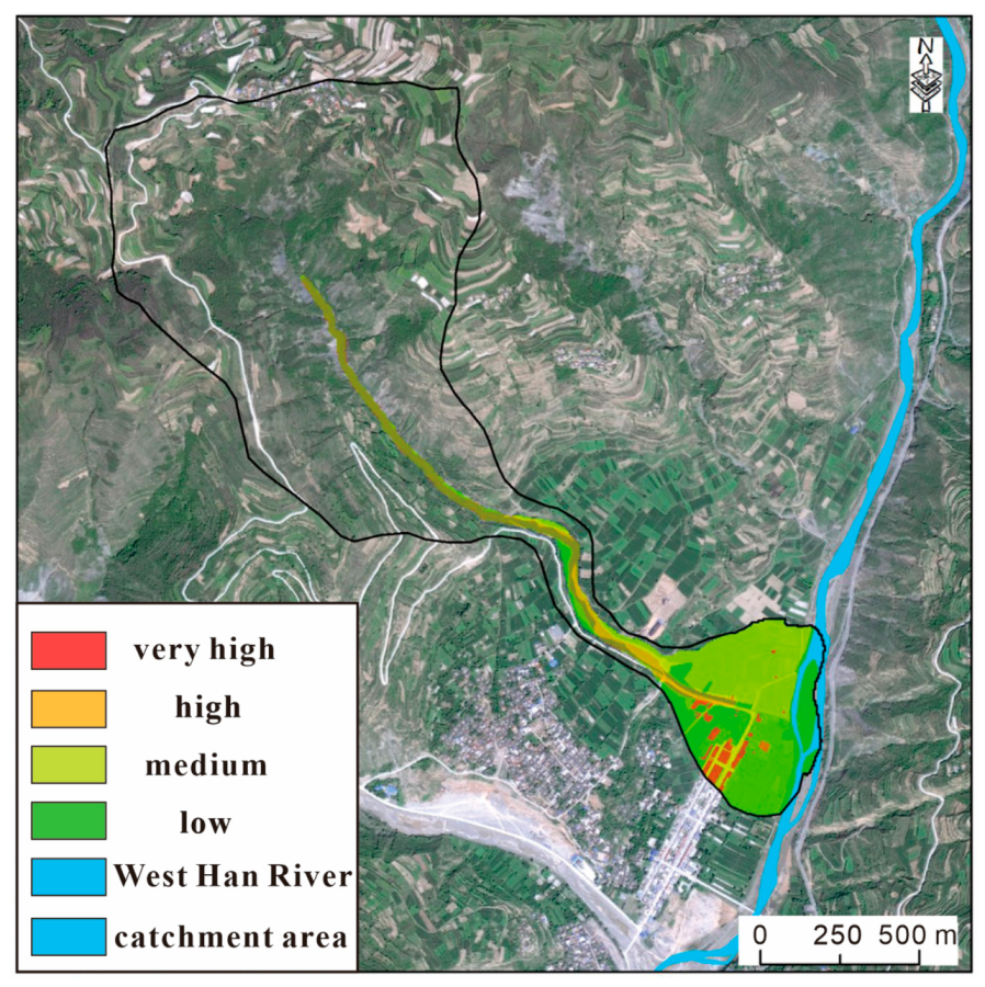
2.2. Wujiagou Debris Flow

The Wujiagou debris flow is located on the right bank of the West Han River in Longlin Town, Lixian County, with the basin planform in the shape of a “slender funnel”. The basin area is about 1.56 km², the main ditch is 3715 m long, the average width is 600 m, the highest point of the basin is 1801 m above sea level, and it joins the West Han River at 1285 m above sea level. The relative height difference of the basin is 516 m, and the average longitudinal drop is 138.9‰. The upper part of the valley is a deep “V”-shaped valley, and the middle and lower parts are “U”-shaped valleys. The slope of the valley is steep, with an average slope of 35° on both sides, and the profile is convex and linear.

2.3. Overview of Geological Hazards in the Study Area

The main types of geological hazards in the study area include collapses, landslides, and debris flows. A total of 2114 collapses, landslides, and debris flows were found through the field geological survey, including 1173 landslides (55.49%), 509 debris flows (24.08%), and 432 collapses (20.44%). The specific distribution of geological hazards in the study area is shown in Figure 1.

2.4. Overview of Geological Hazards in the Study Area

The data used in this study are mainly from the basic information of the area, and they were combined with the remote sensing image InSAR, aerial photography via UAV, a ground survey, drilling, trenching, integrated physical exploration, and experimental testing. The obtained data are mainly used for (i) extracting the slope, gully density, and specific drop of a debris-flow gully bed, (ii) risk source identification, the disaster-bearing body type, and other interpretations, and (iii) obtaining physical and mechanical indexes such as geotechnical density/capacity, water content/permeability coefficients, and internal friction angles and cohesion for model calculation and analysis. The detailed data sources and formats are shown in

Table 1. Data types and sources.

Base Data	Data Source and Production	Data Format
DEM	Geospatial data used to extract slope, gully density, and specific drop of debris-flow gully bed, etc.	National Geographic Information Center: 5 m × 5 m raster data
DOM/DLG	Land use type data	National Geographic Information Center: 5 m × 5 m raster and vector data
Geological data	Lithological zoning and fracture structure	1:200,000 regional geological map, vector data
Remote sensing data	For risk source identification, disaster-bearing body types, etc.	Interpretation of P-star and UAV data, raster data
Geological disaster data	According to the “Longnan West Han River Basin Disaster Geological Survey” (2019–2021) project database	1:10,000 precision vector data
Rainfall data	Lanzhou central meteorological station and Longnan city geological disaster professional monitoring network	Point cloud (vector) data
Survey and test data	Geotechnical density/capacity, water content/permeability coefficient, and physical and mechanical indicators such as angle of internal friction and cohesion for model calculation and analysis	Text data format

.

3. Methods

3.1. Hazard Evaluation Model

3.1.1. Regional Scale

In this study, nine environmental factors, such as the topographic relief, slope, slope direction, engineering geological rock group, distance from the fault, density of gully distribution, normalized vegetation index, degree of human engineering activities, density of debris materials, such as debris-flow sources, etc., were selected, and a 25 m × 25 m resolution raster cell was used as the basic evaluation unit of geological hazard susceptibility in the study area. On this basis, a regional geological hazard susceptibility evaluation [45,46] was carried out using the information volume method [47,48] with the combined hierarchical analysis model [49,50].

(1) Information value model.

The informativeness model is a kind of Bayesian probability model that can better integrate the subjective experience of experts and the relevance of disaster-causing elements to geological hazards, and the algorithm is more stable and has a clear connotation. This model typically uses a probability form for quantitative descriptions, which can reflect the contribution size of different disaster-forming elements’ intervals to the formation of geological hazards, and the expression of a geological hazard’s information quantity I_Aj→B is as follows:

$$I_{\mathrm{Aj}\to B}=\ln \frac{P\left(B/A_j\right)}{p\left(B\right)}=\ln \frac{N_j/S_j}{N/S} (j = 1, 2,\dots n)$$

(1)

where I_Aj→B is the amount of information about the occurrence of geohazard B in the jth interval of the corresponding disaster-forming element A, N_j is the area value or number of disaster points of the geohazard in the jth interval in the corresponding disaster-forming element A, S_j is the area of distribution for the jth interval in the disaster-forming element A, N is the total area of distribution or total number of disaster points of regional geological hazards, and S is the total area of the region.

The “positive value” of I_Aj→B indicates that the element interval is favorable to the occurrence of geological hazards, a “negative value” indicates that the element interval is unfavorable to the occurrence of geological hazards, and a “zero value” indicates that the element interval is not favorable to the occurrence of geological hazards. The “0 value” indicates that this factor interval has a medium level of contribution to the formation of geological hazards.

(2) Hierarchical analysis model.

This study adopted hierarchical analysis and GIS spatial analysis to evaluate and zone the vulnerability of geological hazards, and the main processes included the following: (i) determining evaluation units and evaluation factors and determining the weights of each factor and each element using hierarchical analysis; (ii) quantifying the indicators of each evaluation factor and using the normalized numerical transformation method to unify the outline of the quantity; (iii) on the basis of the determination of evaluation index weights and data normalization, using the spatial analysis function of the GIS system for spatial superposition and the statistics of data; and (iv) determining the boundary points of the susceptibility zone via statistical analysis and dividing the evaluation results into different levels so as to complete the geological disaster susceptibility zone map.

3.1.2. Local Scale

The 24 historical debris flows in the Longnan area, also in Gansu Province, were taken as an example. A detailed field survey was conducted to obtain their critical information. Some nonlinear statistical methods [51,52,53], available on the Matlab platform, were used to establish a maximum outflow prediction model for debris flows in the study area and the previous prediction model optimization to improve the construction of different-scale rainfall frequency for the debris-flow activity scale’s quantitative expression. The equation is as follows:

$${\mathrm{v}}_i=0.0182\times p\times {(A_{b}W)}^{0.5903}$$

(2)

where v_i is the maximum flushing-out volume (10⁴ m³) of the mudflow at one time in year i of the rainfall frequency, W is the total amount of loose solids (10⁴ m³) in the mudflow basin, which represents the materials from the source area, A_b is the area of the future mudflow disaster outbreak area (km²), p is the rainfall coefficient, i.e., (i/10) dimensionless, for the rainfall frequency (year) of mudflow of different scales, and its correlation coefficient is R² = 0.92.

An empirical formula proposed by Liu Xilin et al. [54] was used to calculate the maximum mudflow accumulation thickness and length, considering that the rainfall-type mudflows in the study area are generally large in scale, so the mudflow capacity value was also used as the calculation index, and the final improved formula is as follows:

$$l=8.71\times {(v_i\times I\times r_D^4/\log r_D)}^{1/3}$$

(3)

$$d=0.017\times {(v_i\times r_D/(I^2\times \log r_D))}^{1/3}$$

(4)

where l is the predicted maximum accumulation length of a debris flow (m), d is the predicted maximum accumulation thickness of a debris flow (m), v_i is the maximum amount of debris flow in the rainfall frequency for an annual maximum washout (m³), I is the specific drop of a debris-flow gully bed (decimal representation), and r_D is the debris-flow capacitance (g/cm³).

3.1.3. Site Scale

This time, the FLO-2D fluid model [55,56,57] was mainly used to numerically simulate and analyze the Wujiagou mudflow. The model is based on a non-Newtonian fluid model and finite difference method to solve the motion process, so it is commonly used for debris-flow motion analysis and flood hazard management. The model continuum equation is as Equation (5), and the equations of motion are as Equations (6) and (7):

$$\frac{\partial h}{\partial t}+\frac{\partial (uh)}{\partial x}+\frac{\partial (uh)}{\partial y}=I$$

(5)

$$s_{fx}=s_{ox}-\frac{\partial h}{\partial x}-\frac{\partial u}{g\partial t}-u\frac{\partial u}{\partial x}-v\frac{\partial y}{g\partial y}$$

(6)

$$s_{fy}=s_{oy}-\frac{\partial h}{\partial x}-\frac{\partial u}{g\partial t}-u\frac{\partial u}{\partial x}-v\frac{\partial y}{g\partial y}$$

(7)

where h is the flow depth of the debris-flow fluid (m), I is the hydraulic slope drop (%), u represents the average flow velocity of the fluid in the horizontal direction (m/s), and v represents the average flow velocity of the fluid in the vertical direction (m/s). S_fx and S_fy are frictional slopes (%); S_ox and S_oy are bed-bottom slopes (%), and they can be computed from the DEM data in the FLO-2D software version 6.0, whereas then, the frictional slopes are obtained from equations. Equations (6) and (7) are the momentum equations representing the dynamic balance.

3.2. Vulnerability Evaluation Methods

3.2.1. Regional Scale

Vulnerability evaluation first identifies and classifies elements at risk, which is mainly achieved by means of data collection and the analysis of the evaluation area, a field survey, high-resolution remote sensing interpretation, large-scale topographic mapping, or aerial photogrammetry. The main contents include population distribution, buildings, roads, land use, and four 4 other major categories.

The social vulnerability sub-indicators are mainly population distribution; for convenience, population distribution density was used and given a corresponding loss probability, and finally, social vulnerability was expressed through monetary quantity. The following formula was used for these calculations: social vulnerability is the product of the number of people per square meter, the average individual value, and the average probability of damage.

Physical vulnerability: The potential economic loss of different base buildings and land use types of elements at risk was selected as the sub-index for evaluation. The vulnerability of residential buildings can be calculated using the following formula, and so on for other building types: the total value of a house is the product of the cost per square meter of its construction and floor area and the interior and other property. The vulnerability of a civil house is the product of the total value of the civil house and overall damage probability. In addition, the vulnerability of elements at risk, such as highways, bridges, and drylands, was calculated according to the following formula: road vulnerability is the product of the cost per square meter, the area of the road, and the probability of damage.

The vulnerability of geological hazards in the work area was evaluated by constructing a model using the ArcGIS software version 10.2. The economic value of the vulnerability of different types of elements at risk was spatially superimposed under the ArcGIS platform to obtain the vulnerability zoning map of the work area, and the total economic value in each grid was subjected to a normalization process as follows:

$$V=0.1+\frac{X-X\min }{X\max -X\min }\times 0.9$$

(8)

where V is the normalized value of vulnerability, and X_max and X_min are the maximum and minimum values of economic value in the raster data. According to the actual situation of the evaluation area, combined with past disaster losses, the normalized vulnerability index of the disaster-bearing body was divided into 4 levels: when 0 < V ≤ 0.25, the disaster-bearing body has very low vulnerability; when 0.25 < V ≤ 0.45, the disaster-bearing body is low-vulnerability; when 0.45 < V ≤ 0.75, the disaster-bearing body is medium-vulnerability; when 0.75 < V ≤ 1.0, the disaster-bearing body is high-vulnerability. Finally, the vulnerability evaluation map of the disaster-bearing body under different working conditions in the West Han River Basin was formed.

3.2.2. Local Scale

Vulnerability scoring indexes mainly consider the value of elements that are at risk and threatened due to geohazards in key areas and their resilience to disasters, including eight indexes of fixed people, mobile people, buildings, line facilities, others, and vulnerability. The scoring indexes are based on the type of geological hazards, characteristics, development geological conditions, and the types of elements at risk in different mountainous key areas, etc. Different combinations of scoring indexes should be selected to make the evaluation results of the slope risk classification system in mountainous key areas more realistic.

The vulnerability score is composed of two parts, namely weight and the following factors:

$$B={\displaystyle \sum X_i{Y}_i}$$

(9)

where X_i indicates different factors under each category, Y_i indicates the weight of each factor, and the total score of each factor is summed up to get the vulnerability-grade score. A slope-by-slope survey was conducted to obtain a slope vulnerability assessment score sheet for the circled slope. Based on the results of the slope vulnerability survey, the natural interval method was used to classify the hazards into four levels, including very high vulnerability, high vulnerability, medium vulnerability, and low vulnerability.

3.2.3. Site Scale

Different elements at risk have different damage probabilities due to different structures and functions. The probability of possible damage in the high-risk area was set to 80%, the probability of possible damage in the high-risk area to 60%, the probability of possible damage in the medium-risk area to 40%, and the probability of possible damage in the low-risk area to 20%. Finally, on the basis of type identification, quantity range extraction, the field survey and verification, and the statistical analysis of the value accounting of elements at risk in the evaluation area, the economic value of the vulnerability of different types of elements at risk was calculated via spatial superposition on the ArcGIS platform to obtain the vulnerability zoning map of the study area.

3.3. Risk Assessment Methods

3.3.1. Regional Scale

Based on the results of geological hazard and vulnerability analysis, the risk value of each evaluation unit under different precipitation working conditions was calculated according to the definition of hazard risk.

$$R=H\times V\times P_i$$

(10)

where R is the value of the risk index of the evaluation unit, H is the value of the hazard index of the evaluation unit, V is the value of the vulnerability index of the evaluation unit, and P_i is the probability of geohazard occurrence under different precipitation working conditions.

Before calculation, all kinds of indices in the formula had to be normalized, and their normalization method was as follows:

$$H`=(H-H_{\min })/(H_{\max }-H_{\min })$$

(11)

$$V`=(V-V_{\min })/(V_{\max }-V_{\min })$$

(12)

where H` is the normalized value of a hazard, H is the value of the hazard index, H<sub>max</sub> and H<sub>min</sub> are the maximum hazard value and minimum hazard value, respectively, v` is the normalized value of vulnerability, V is the value of the vulnerability index, and V_max and V_min are the maximum vulnerability value and minimum vulnerability value, respectively.

The P_i calculation method uses the previous Longnan mountain geological disaster statistics sample as an example in the completion of the regional geological disaster risk zoning, based on the use of the logistic regression statistical model to determine the spatial and temporal probability of geological disaster risk P_i [58]. The values are 0.72 for the 100-year-return-period (100a) rainfall condition, 0.23 for the 50-year-return-period (50a) rainfall condition, and 0.08 for the 20-year-return-period (20-a) rainfall condition.

After determining the values of normalized H, normalized V, and P_i, the risk probability at each unit was calculated in ArcGIS 10.2, and the values ranged from 0 to 1; 0 means no risk, and 1 means the highest risk. Then, the natural break method was utilized to separate the risk value into four different levels: very high risk (0.697–1), high risk (0.538–0.697), medium risk (0.356–0.538), and low risk (0–0.356).

3.3.2. Local Scale

The risk of regional geohazards was evaluated by combining qualitative and quantitative methods, dividing the investigation area into several evaluation units, analyzing the danger and vulnerability of each evaluation unit, determining the risk level of each evaluation unit according to the risk evaluation matrix (

Table 2. Qualitative analysis and evaluation table of geological disaster risk.

Risk Classification	Very High Vulnerability	High Vulnerability	Medium Vulnerability	Low Vulnerability
Very high hazard	H	H	M	L
High hazard	H	M	M	L
Medium hazard	M	M	L	L
Low hazard	L	L	L	VL

Note: H—very high risk; M—high risk; L—medium risk; VL—low risk.

), and forming a risk evaluation and zoning map.

$$R=H\times V$$

(13)

where R represents the expected value of the loss of people and property or damage to social and economic activities caused due to geological hazards, H denotes the hazard, the probability of occurrence of geological hazards within a certain period of time, and V indicates vulnerability, the degree of damage caused to the threatened object due to the occurrence of geological hazards with a certain probability. This definition reflects the natural and social nature of geological hazards: a larger H indicates that it is more dangerous, while a larger R indicates a greater risk.

3.3.3. Site Scale

After normalizing the risk and vulnerability of the Wujiapo debris flow, the calculation method for risk evaluation was used to analyze the risk probability of geohazards under different working conditions, and the comprehensive risk degree of the Wujiapo debris flow was obtained by multiplying the normalized data for the hazard of geohazard chain and the normalized data for the vulnerability of the disaster-bearing body.

In the risk classification, according to the characteristics of the geological environment of a single geological disaster, the characteristics of mudflow development, the socio-economic situation, the results of the investigation of the threat to people and properties due to a geological disaster in recent years, and the preliminary results of the above comprehensive analysis, the natural breakpoint method and characteristic points were selected to grade the evaluation results, and the risk degree was generally classified as very high-risk (0.697~1), high-risk (0.538~0.697), medium-risk (0.356~0.538), and low-risk (0~0.356).

4. Results

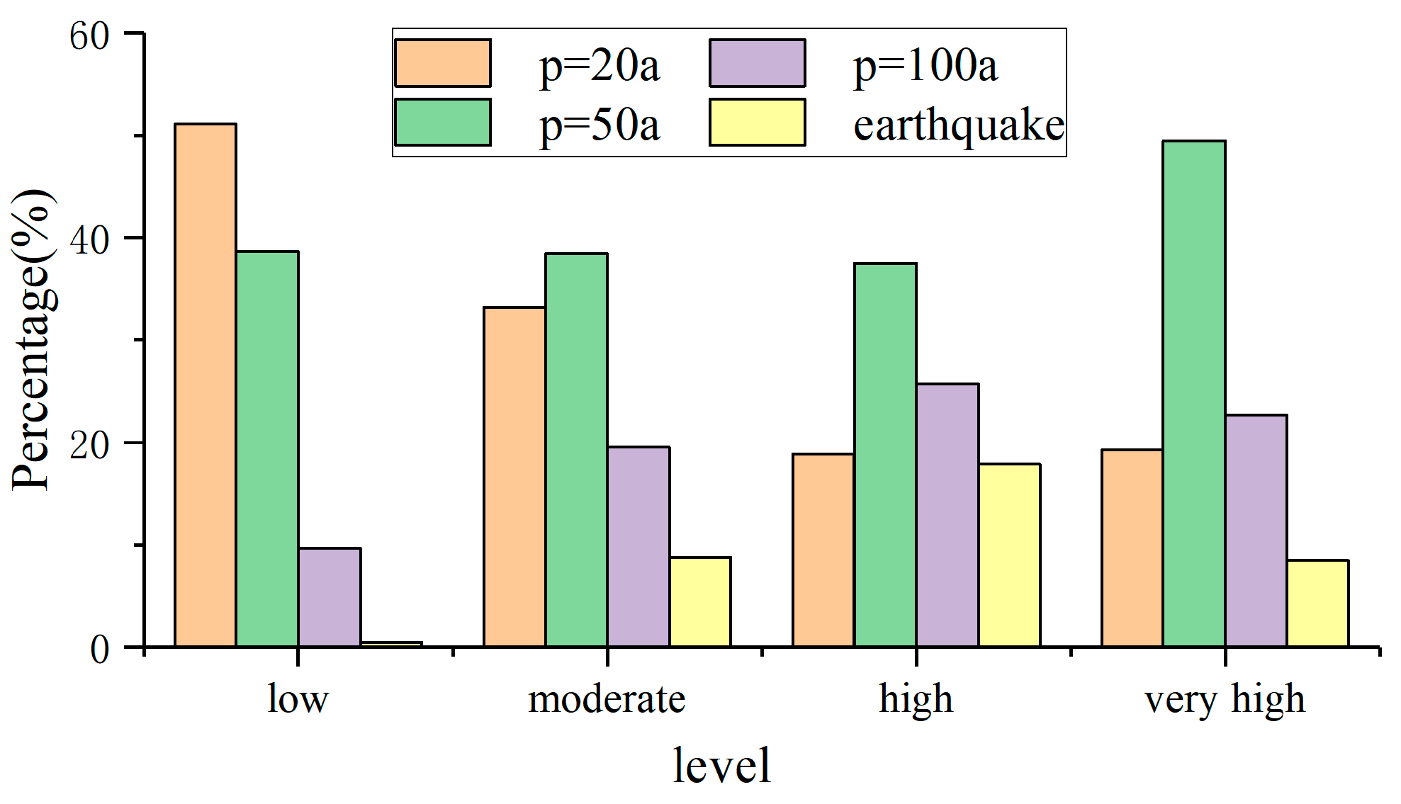
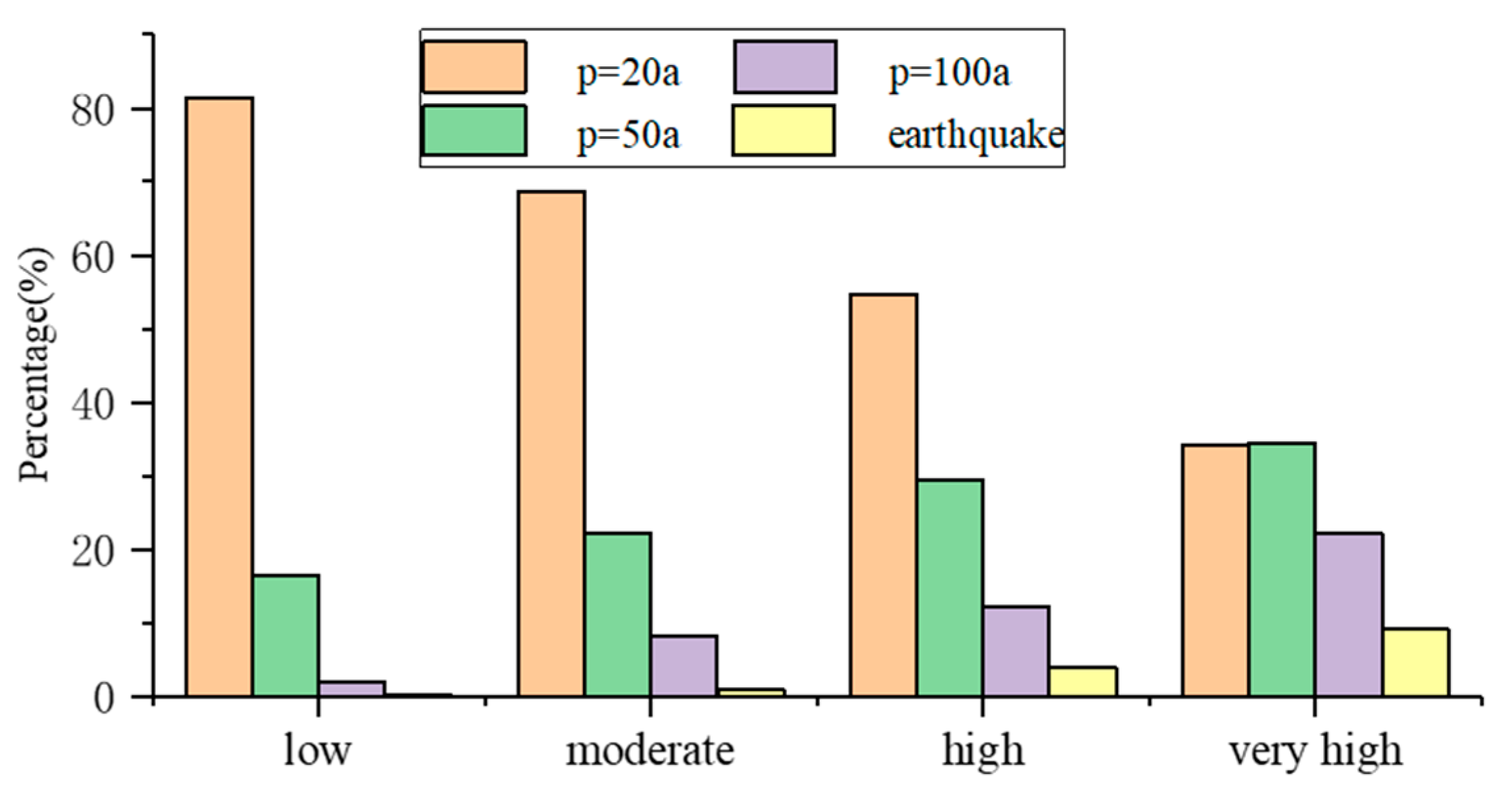
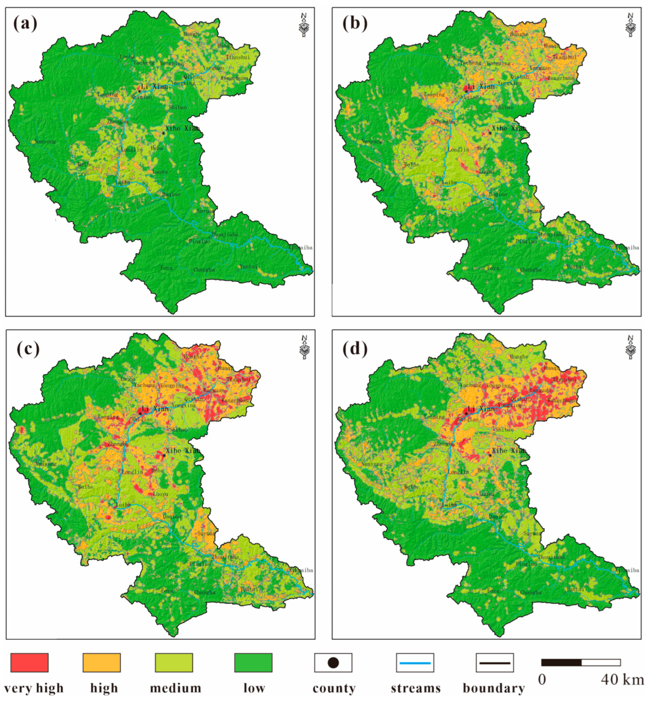
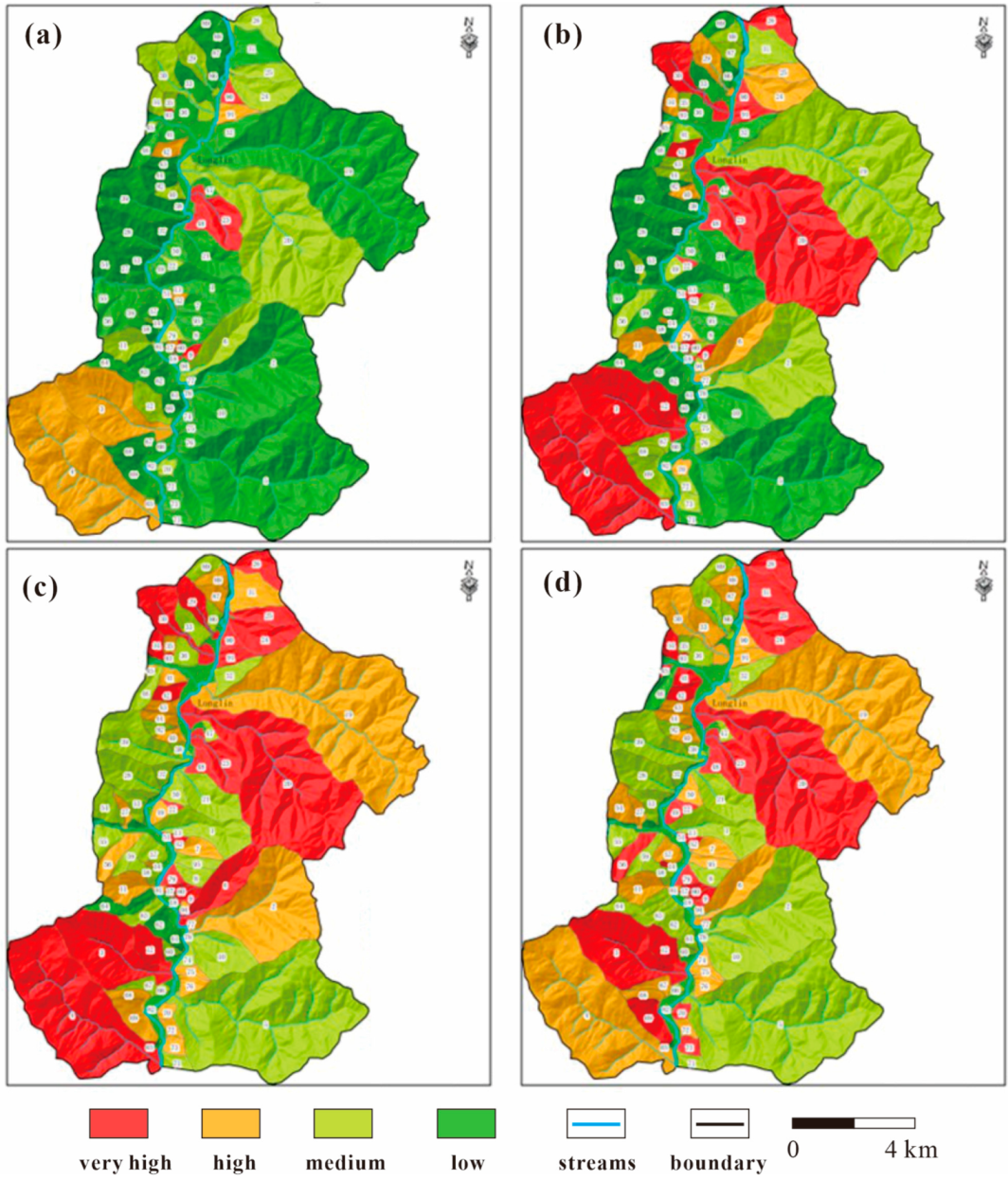
4.1. Risk Results and Assessment at a Regional Scale

The results of the geohazard risk assessment at the regional scale under seismic conditions (p = 50a) and under different precipitation conditions are shown in Figure 2. Spatially, the hazard was higher in the central part when p = 20a, and it increased in the northeast as the rainfall recurrence period increased to 100a, and the hazard risk was particularly severe in the northeast under seismic conditions.

The percentages of each hazard level under different conditions were summarized, and the results (Figure 3) showed that, as the rainfall return period increased from 20a to 100a, the total very high- and high-hazard areas in the study region increased from 10.19% to 43.60%, the medium area remained almost unchanged, and the low-hazard area decreased significantly from 51.12% to 18.86%; at p = 50a, the total very high- and high-hazard areas for geological hazards in the study area increased slightly from 28.36% to 31.21%, the medium-hazard areas increased by 11.04%, and the low-hazard areas decreased by 13.90% from no to extreme seismic conditions. In general, the risk is higher in the central and northeastern parts of the West Han River watershed, while it is lower in the southern and northwestern parts, and storm conditions cause a greater risk than seismic conditions.

The results of a geohazard vulnerability evaluation under seismic conditions (p = 50a) and different precipitation conditions are shown in Figure 4. Spatially, the overall regional vulnerability was low at p = 20a and 50a, and under p = 100a and seismic conditions, the vulnerability was larger in the central and northeastern parts, while the vulnerability grew in some scattered areas in the south.

The results (Figure 5) show that, as the rainfall return period increases from 20a to 100a, the total very high- and high-vulnerability areas in the study area increased from 2.15% to 15.95%, the medium-vulnerability areas increased by 12.76%, and the low-vulnerability areas decreased significantly from 81.31% to 54.75%. At p = 50a, there was a significant increase in the total very high- and high-vulnerability areas of geological hazards in the study region from no to extreme seismic conditions; from 9.19% to 31.37%, an increase of 12.35% in medium-vulnerability areas and a decrease of 34.53% in low-risk areas were observed. In general, the regional vulnerability was low under lower rainfall return period conditions, and under heavy rainfall and seismic conditions, the whole area’s vulnerability increased, and it was the greatest in the central and northeastern regions.

The results of the geohazard risk evaluation under seismic conditions (p = 50a) and different precipitation conditions are shown in Figure 6. Spatially, the region is safer under the 1-in-20-year rainfall condition; there was a small increase in riskiness in the central and northeastern parts under the 1-in-50-year rainfall condition, and the riskiness was higher in the central and northeastern parts under the 1-in-100-year precipitation condition and extreme earthquake condition.

The results (Figure 7) show that, as the rainfall return period increases from 20a to 100a, the total very high- and high-risk geological hazards in the study area increased from 2.42% to 24.18%, the medium area increased by 18.89%, and the low-risk area decreased significantly by 40.64%; at p = 50a, from no seismic conditions to extreme seismic conditions, the total area of the very high- and high-risk geological hazards in the study region increased. Under extreme seismic conditions, the total area of very high- and high-risk geological hazards in the study region underwent a significant increase from 11.56% to 21.84%, the medium-risk area had almost no change, and the low-risk area decreased by 10.78%. In general, the overall riskiness evaluation was similar to the vulnerability evaluation, indicating that vulnerability has a greater impact on riskiness than hazards.

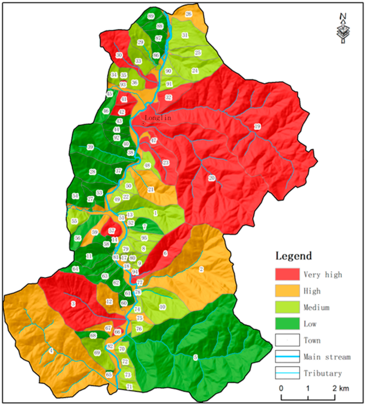
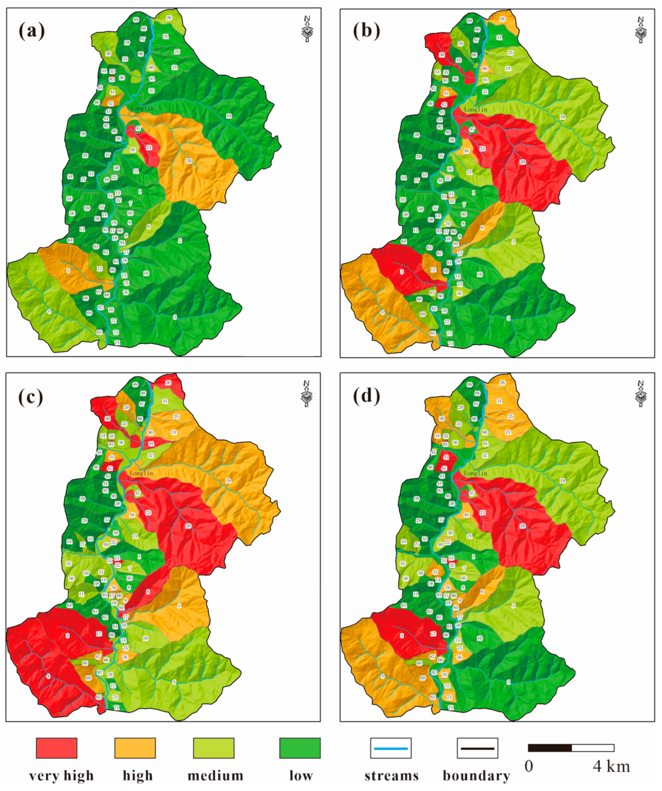
4.2. Risk Results and Assessment at Local Scale

The results of the geohazard risk evaluation under seismic conditions (p = 50a) and under different precipitation conditions are shown in Figure 8. Spatially, there were only three very high-risk areas under the 20-year rainfall conditions, eight very high-risk areas under the 50-year rainfall conditions, two of which were large, and more than ten very high-risk areas under both the 100-year precipitation conditions and extreme earthquake conditions. The southwest was always above the high danger zone, and when the rainfall scale was slightly larger, the northeast was also above the high danger zone.

The results (

Table 3. Geological hazard evaluation grading table for the key area of the Longlin-Leiba Town section.

Frequency	Evaluation Result Grading Area (km2)				Evaluation Result Grading Ratio (%)
	Low Zone	Medium Zone	High Zone	Very High Zone	Low Zone	Medium Zone	High Zone	Very High Zone
20-year event	64.32	21.06	13.76	2.17	63.49	20.79	13.58	2.14
50-year event	35.82	28.66	6.79	30.04	35.36	28.29	6.70	29.65
100-year event	5.27	30.86	29.69	35.49	5.20	30.46	29.31	35.03
Seismic conditions	4.41	36.12	35.05	25.73	4.35	35.65	34.60	25.40

) summarize the percentages of each hazard level under different conditions and show that, as the rainfall return period increased from 20a to 100a, the total very high- and high-hazard areas in the study region increased significantly from 15.42% to 64.34%, the medium area increased by 9.67%, and the low-hazard area decreased significantly by 58.29%; at p = 50a, from no earthquake conditions to extreme seismic conditions, the total very high- and high-risk areas for geological hazards in the study region increased from 36.35% to 60%, the medium-risk area increased by 7.36%, and the low-risk area decreased by 31.01%. In general, the riskiness was higher in the southwest and northeast, and even more so in the southeast and west, and the seismic and storm conditions had comparable effects on the riskiness.

The results of the qualitative evaluation of the geological hazard susceptibility by slope unit are shown in Figure 9. The eastern, northeastern, and southwestern parts of the focal area were all extremely high and had highly susceptible slopes, with a small portion of extremely high-susceptibility areas in the north and low susceptibility in the west and southeast.

The results of the geohazard risk evaluation under different working conditions are shown in Figure 10. It can be found that, spatially, when the rainfall return period was small, the risk was higher in the southwest and central parts of the study area; however, when the precipitation conditions increased to a 100-year event, some slope units in the northern part of the study area also increase from medium risk to a high risk level. However, the risk in the western and southeastern parts of the study area was consistently lower because their hazard and susceptibility assessments were both relatively low.

The percentages of each risk level under different scenarios were further summarized, and the results (Figure 11) show that, as the rainfall return period increased from 20a to 100a, the very high- and high-risk areas of geological hazards increased significantly from 16.23% to 57.33%, the medium areas increased by 13.96%, and the low-risk areas decreased significantly with a change of up to 55.04%; at p = 50a, the total very high- and high-risk areas for geological hazards in the study region increased from 30.89% to 37.29%, the medium-risk areas increased by 3.23%, the and low-risk areas decreased by only 9.63% from no to extreme seismic conditions. Thus, the overall risk level of the study area is more responsive to storm conditions. It is also important to note that the central slope unit (No. 23) was consistently at a very high risk level, and units No. 20 and No. 3 were consistently at a high or very high risk level in all working conditions, so these areas should be further investigated and monitored with emphasis.

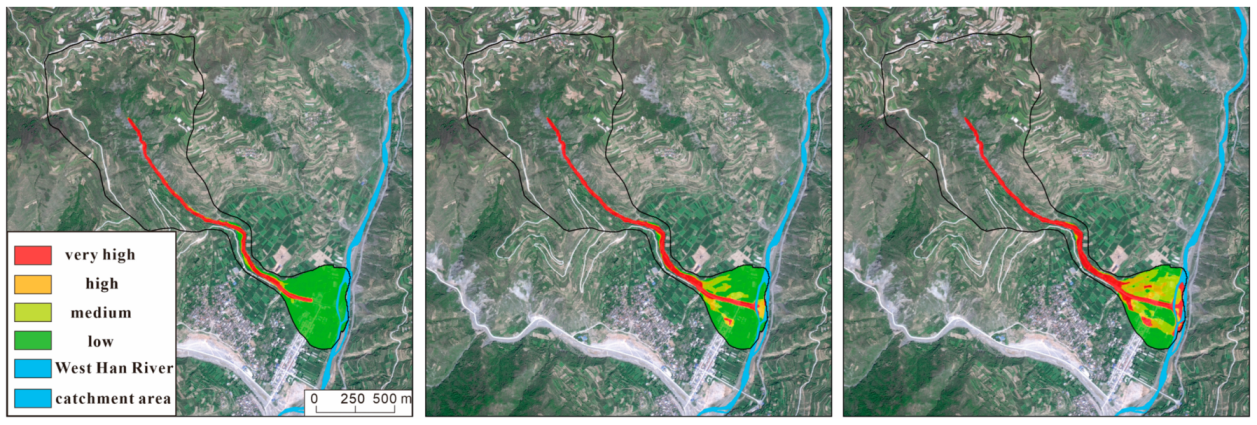
4.3. Risk Results and Assessment for Wujiagou Debris Flow

The FLO-2D simulation results for the Wujiagou debris flow are shown in Figure 12, and the simulation accuracy coefficients are 81.38% (20-year event), 75.53% (50-year event), and 86.74% (100-year event) for the three working conditions, indicating that the simulation results are good. From the figure, it can be found that the debris-flow trench has always belonged to the very high-danger zone, regardless of the working conditions, the flow velocity gradually decreases as the debris flows downward, and the accumulation piles up in the trench valley location, forming a low-danger zone. In the lateral comparison, the gully channel has been in the very high-danger area, and with the increase in the rainfall recurrence period, the accumulation area has been upgraded from low danger to high danger. With the increase in the rainfall recurrence period from 20a to 100a, the proportion of the very high- and high-hazard areas increased from 20.88% to 50.24%, the medium-hazard area increased by 19.80%, and the low-hazard area decreased by 49.15%.

The results of debris-flow susceptibility evaluation are shown in Figure 13. It can be found that the susceptibility was low because there were fewer properties at the gully, the northern part belonged to the medium-susceptibility zone at the debris-flow accumulation, and most of the southern part belonged to the low-susceptibility zone, but a small part of the very high-susceptibility zone appeared.

The results of the debris-flow risk evaluation show (Figure 14 and Figure 15) that, spatially, the risk was more similar to the vulnerability, although the risk was high at the gully, but there was not much property damage, which made the risk greatly reduced; there were more properties at the pile-up, but the risk was less, so the overall risk was also small, and there were only small very high-risk areas. In terms of time, as the rainfall recurrence period increased from 20a to 100a, the very high- and high-risk areas increased from 6.97% to 14.27%, the medium-risk areas increased by 31.54%, and the low-risk areas decreased by 38.84%.

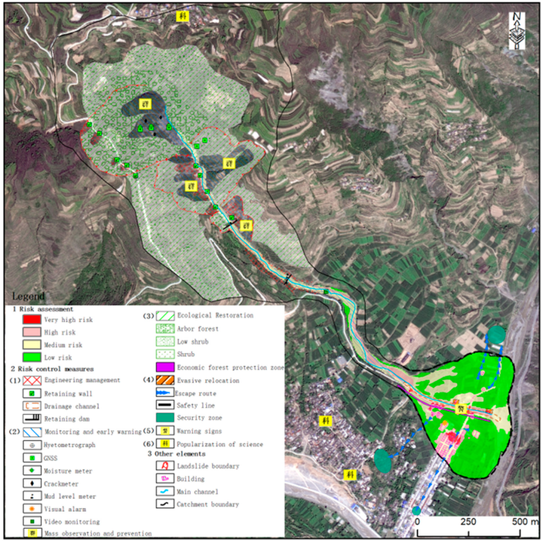
4.4. Multi-Scale Geological Disaster Risk Control

Geological disaster risk consists of the possibility of the occurrence of (hazard) and possible consequences (vulnerability) of geological disasters, and its essence is to express the uncertainty of disasters through probability. Reducing the risk of the hazard body, decreasing the encounter probability between the hazard-causing body and the hazard-bearing body, and improving the damage resistance of the hazard-bearing body can effectively reduce the risk of geological hazards. The evaluation methods and accuracy of geological hazard risk evaluation vary from scale to scale, and the degree of supporting risk control also varies. Hence, recommendations of geological hazard risk control are introduced using three spatial scales in this section.

At the regional scale, the risk sources in the hilly loess area in the upper reaches of West Han River are a loess landslide and a loess mudflow. The main risk control measures are to reduce the impact of production and living activities on geological hazards and control the hazard risk. Regarding the middle reaches of the West Han River, the risk sources are large and medium-sized gully storm-type debris flows and mound landslides, which are large in scale and strong in destructive power. The main measures are to reduce the encounter probability between the disaster itself and elements at risk. For example, the centralized resettlement of threatened residents and the strengthening of early warnings are potential measures. In view of the current situation of geological disaster development and the spatial distribution of danger and risk in the West Han River watershed, it is appropriate to adopt the general policy of “prevention as a prerequisite, monitoring and early warning as the main focus, engineering prevention and control as a supplement, long-term biological protection and avoidance of key disasters”. Overall, in basin or regional geological disaster risk control, it is necessary to conduct risk analysis and risk mitigation cost analysis according to the characteristics of geological disaster development, danger, and the hazard in different areas and determine the combination of measures in order to achieve the optimal effect of risk prevention and control on the basis of economic and reasonable approaches.

Based on the risk mapping and results at the local scale, the comprehensive risk control and management methods for geological hazards at Longlin-Leiba Town can be obtained. The specific measures include natural ecological restoration and artificial intervention restoration in slope areas and low- and medium-risk areas, engineering treatments for very high-risk hazard sites, monitoring and early warning, and six other categories. The specific control recommendations are shown in Figure 16. The details for these measures can be described as follows:

(i) Engineering management is mainly for geological hazards or hidden spots with poor stability threatened due to towns and surrounding infrastructure and residents, threatened due to a large population, and difficult to relocate. (ii) Monitoring and early warning are mainly for geological hazards of medium–large scale, threatening property and population, hazards that are difficult to manage, and hazards with a high economic cost of management. (iii) Mass observation and mass prevention are mainly for geological hazards or hidden spots with a small-to-medium scale, poor stability, or medium-to-high susceptibility and unstable future development trends with a clear threat to people. (iv) The popularization of science is mainly for geological hazards or hidden spots with low vulnerability to geological hazards, threatening farmland and rivers. (v) Establishing warning signs is mainly for geological hazards or hidden spots that only threaten roads. (vi) The ecological restoration in an ecological engineering zone is mainly located in areas below a high or medium risk, where there is no geological hazard zone that threatens people’s lives and properties or has a greater impact on major engineering construction. A natural restoration area is mainly located within the medium–low-risk area, and the land use type is mainly within areas of farmland and mature forests.

Regarding the Wujiagou debris flow, according to the geological hazard body, the characteristics of the disaster-bearing body, and the deployment status of prevention and control measures, one or more types of risk control measures can be proposed. Specifically, these measures include engineering management measures, ecological restoration, evasive relocation, monitoring and early-warning means, the popularization of science, and warning signs. The above risk control measures are characterized by a combination of points, lines, and surfaces. The proposed risk control measures for the Wujiagou debris flow under different rainfall conditions are shown in Figure 17 and Figure 18.

5. Discussion

The modeling uncertainties and limitations of the present study were mainly associated with three aspects: (i) the empirical equations used during the hazard assessments, (ii) the vulnerability assessments, and (iii) the risk zonation method for the zonation mapping.

Firstly, an event-based, empirical approach was used to analyze the potential kinematic process of debris flows under a specific condition. The purpose of this was to determine the influencing area for the debris flow at the local scale. The empirical equations (Equations (2) and (3)) applied during this procedure allowed us to directly calculate the maximum flushing-out volume, movement distance, and accumulation depth of the debris flow. It should be noted that the coefficients used in these equations should be assessed more strictly because they inherited the characteristics of historical events, not those occurring in the test area. However, the historical events had similar geological contexts as the debris flows in the study area (they were in the same province), and the correlation coefficient indicated that the fitting result was not bad. Similar empirical approaches were also observed in some of the other literature regarding the modeling for debris flows [59,60]. Hence, this led us to conclude that predicting the hazard of debris flows quantitatively, using the empirical method, may be feasible for regional studies, especially the debris-flow events that had not happened yet. Similar conditions also existed when it came to the vulnerability assessment. As reported in many previous studies [38,41,61], this component may provide the highest uncertainty for risk assessment, as it is complicated to estimate vulnerability quantitatively, and many factors should be taken into account. In the present study, a semi-quantitative model was applied to estimate the vulnerability of elements at risk due to the geohazard. This was close to an empirical method because high subjectivity was included. The development of physical models based on vulnerability curves may be of high interest since they could be a potential solution to this issue. Some efforts have been made on this topic [30,31], but they were not the case in this study.

After determining the hazard and vulnerability at the local scale, the risk matrix was used to define the risk level and zonation. Obviously, this step also mixed uncertainties with risk mapping. However, the risk results’ zonation via this procedure presented a more relative risk level, rather than an absolute level. This means that users should consider the final mapping from multiple views. On one hand, the risk map may have inherited a certain amount of uncertainties from previous steps, hence reducing the results’ accuracy. On the other hand, the obtained zonation can indeed represent the actual potential risk posed due to geohazards, which can provide a foundation for risk mitigation and reduction. Therefore, although some improvements can be made, uncertainty in risk assessment will always occur. Honestly informing the user of the associated limitations is important, instead of ignoring them [62].

Last but not least, the return period of rainfall was utilized in determining the scenarios of risk assessment in this study. It should be noted that this is not standard, as the well-known IPCC report recommended using the standard levels of probability, rather than the return period of triggering events. However, this method has been widely applied for case studies in China [38,63]. So, we continued this practice in the present study. Additionally, we also observed a similar method in some international publications in other countries [64,65].

6. Conclusions

The risk assessment of geohazards has been widely implemented at various scales, but limited efforts have been made to compare the framework and detailed procedures at multiple scales. In this study, the risk and vulnerability assessment of geological hazards was carried out using different scales in the West Han River watershed of Gansu Province, China, and a risk zoning map was ultimately obtained. Our main objective was to present the difference during a geohazard risk assessment within the scope of the framework of GIS techniques. The hazard assessment mainly utilized GIS-based evaluation models and numerical simulation methods, whereas the vulnerability assessment was mainly associated with empirical methods.

The results indicate that the regional risk in the West Han River watershed is low under low rainfall-recurrence conditions, and the risk is higher in the central and northeastern parts of the watershed under heavy rainfall and earthquake conditions, which require early warning and prevention. The overall risk level of the study area in the Longlin-Leiba Town section responds more significantly to heavy rainfall conditions, with higher risk in the southwestern, central, and northeastern parts of the region and higher risk in the north under extreme weather. In Wujiagou, although the hazard value is high at the trench, the amount of property is small, thus making the final risk not high. Regarding the accumulation area, the property value is higher, but the hazard value is lower. Hence, the obtained risk level is also low.

In general, the present study has shown a specific example and procedure regarding risk assessment for geohazards at multiple scales, which can provide scientific references for risk management and a reduction in geohazards in areas with similar conditions.

References

1. Catani, F.; Casagli, N.; Ermini, L.; Righini, G.; Menduni, G. Landslide hazard and risk mapping at catchment scale in the Arno River basin. Landslides 2005, 2, 329–342. [Google Scholar] [CrossRef]
2. Calvello, M.; Papa, M.N.; Pratschke, J.; Crescenzo, M.N. Landslide risk perception: A case study in Southern Italy. Landslides 2016, 13, 349–360. [Google Scholar] [CrossRef]
3. Corominas, J.; van Westen, C.J.; Frattini, P.; Cascini, L.; Malet, J.; Fotopoulou, S. Recommendations for the quantitative analysis of landslide risk. Bull. Eng. Geol. Environ. 2013, 73, 209–263. [Google Scholar] [CrossRef]
4. Chen, L.; van Weatern, C.J.; Hussin, H.; Ciurean, R.L.; Turkington, T.; Chavarro-Rincon, D.; Shrestha, D.P. Integrating expert opinion with modelling for quantitative multi-hazard risk assessment in the Eastern Italian Alps. Geomorphology 2016, 273, 150–167. [Google Scholar] [CrossRef]
5. Wu, C.Y.; Chen, S.C. Integrating spatial, temporal, and size probabilities for the annual landslide hazard maps in the Shihmen watershed, Taiwan. Nat. Hazards Earth Syst. Sci. 2013, 13, 2353–2367. [Google Scholar] [CrossRef]
6. Hürlimann, M.; Guo, Z.; Puig-Polo, C.; Medina, V. Impacts of future climate and land cover changes on landslide susceptibility: Regional scale modelling in the Val d’ Aran region (Pyrenees, Spain). Landslides 2022, 19, 99–118. [Google Scholar] [CrossRef]
7. Chen, S.C.; Wu, C.Y. Annual landslide risk and effectiveness of risk reduction measures in Shihmen watershed, Taiwan. Landslides 2016, 13, 551–563. [Google Scholar] [CrossRef]
8. Jaiswal, P.; van Western, C.J. Use of quantitative landslide hazard and risk information for local disaster risk reduction along a transportation corridor: A case study from Nilgiri district, India. Nat. Hazards 2013, 65, 887–913. [Google Scholar] [CrossRef]
9. Guo, Z.; Torra, O.; Hürlimann, M.; Medina, V.; Puig-Polo, C. FSLAM: A QGIS plugin for fast regional susceptibility assessment of rainfall-induced landslides. Environ. Model. Softw. 2022, 150, 105354. [Google Scholar] [CrossRef]
10. Guo, Z.; Tian, B.; Li, G.; Huang, D.; Zeng, T.; He, J.; Song, D. Landslide susceptibility mapping in the Loess Plateau of northwest China using three data-driven techniques-a case study from middle Yellow River catchment. Front. Earth Sci. 2023, 10, 1033085. [Google Scholar] [CrossRef]
11. Deschepper, E.; Thas, O.; Ottoy, J.P. Regional residual plots for assessing the fit of linear regression models. Comput. Stat. Data Anal. 2006, 8, 1995–2013. [Google Scholar] [CrossRef]
12. Silva, A.; Brito, J.; Gaspar, P.L. Deterministic Models. In Methodologies for Service Life Prediction of Buildings; Green Energy and Technology; Springer: Cham, Switzerland, 2016; Volume 4, pp. 67–162. [Google Scholar]
13. König, T.; Kux, H.J.H.; Mendes, R.M. Shalstab mathematical model and WorldView-2 satellite images to identification of landslide-susceptible areas. Nat. Hazards 2019, 97, 1127–1149. [Google Scholar] [CrossRef]
14. Tien, B.D.; Tran, H.T.; Bui, X.N. (Eds.) Proceedings of the International Conference on Innovations for Sustainable and Responsible Mining; Springer: Cham, Switzerland, 2021; Volume 108, pp. 210–229. [Google Scholar]
15. Nie, Y.; Li, X.; Xu, R. Dynamic hazard assessment of debris flow based on TRIGRS and flow-R coupled models. Stoch. Environ. Res. Risk Assess. 2022, 36, 97–114. [Google Scholar] [CrossRef]
16. Gatto, M.P.A.; Lentini, V.; Montrasio, L.; Castelli, F. A simplified semi-quantitative procedure based on the SLIP model for landslide risk assessment: The case study of Gioiosa Marea (Sicily, Italy). Landslides 2023, 20, 1381–1403. [Google Scholar] [CrossRef]
17. Medina, V.; Hürlimann, M.; Guo, Z.; Lloret, A.; Vaunat, J. Fast physically-based model for rainfall-induced landslide susceptibility assessment at regional scale. Catena 2021, 201, 105213. [Google Scholar] [CrossRef]
18. Sezer, E.A.; Nefeslioglu, H.A.; Osna, T. An expert-based landslide susceptibility mapping (LSM) module developed for Netcad Architect Software. Comput. Geosci. 2017, 98, 26–37. [Google Scholar] [CrossRef]
19. Guo, Z.; Tian, B.; He, J.; Xu, C.; Zeng, T.; Zhu, Y. Hazard assessment for regional typhoon-triggered landslides by using physically-based model -A case study from southeastern China. Georisk Assess. Manag. Risk Eng. Syst. Geohazards 2023, 17, 740–754. [Google Scholar] [CrossRef]
20. Remondo, J.; Bonachea, J.; Cendrero, A. A statistical approach to landslide risk modelling at basin scale: From landslide susceptibility to quantitative risk assessment. Landslides 2005, 2, 321–328. [Google Scholar] [CrossRef]
21. Reichenbach, P.; Rossi, M.; Malamud, B.D.; Mihir, M.; Guzzetti, F. A review of statistically-based landslide susceptibility models. Earth-Sci. Rev. 2018, 180, 60–91. [Google Scholar] [CrossRef]
22. Pradhan, B. A comparative study on the predictive ability of the decision tree, support vector machine and neuro-fuzzy models in landslide susceptibility mapping using GIS. Comput. Geosci. 2013, 51, 350–365. [Google Scholar] [CrossRef]
23. Guo, Z.; Tian, B.; Zhu, Y.; He, J.; Zhang, T. How do the landslide and non-landslide sampling strategies impact landslide susceptibility assessment?—A case study at catchment scale from China. J. Rock. Mech. Geotech. Eng. 2024, 16, 877–894. [Google Scholar] [CrossRef]
24. Althuwaynee, O.F.; Pradhan, B.; Park, H.J.; Lee, J.H. A novel ensemble decision tree-based CHi-squared Automatic Interaction Detection (CHAID) and multivariate logistic regression models in landslide susceptibility mapping. Landslides 2014, 11, 1063–1078. [Google Scholar] [CrossRef]
25. Goetz, J.N.; Brenning, A.; Petschko, H.; Leopold, P. Evaluating machine learning and statistical prediction techniques for landslide susceptibility modeling. Comput. Geosci. 2015, 81, 1–11. [Google Scholar] [CrossRef]
26. Zeng, T.; Guo, Z.; Wang, L.; Jin, B.; Wu, F.; Guo, R. Tempo-Spatial Landslide Susceptibility Assessment from the Perspective of Human Engineering Activity. Remote Sens. 2023, 15, 4111. [Google Scholar] [CrossRef]
27. Li, Z.; Nadim, F.; Huang, H.; Uzielli, M.; Lacasse, S. Quantitative vulnerability estimation for scenario-based landslide hazards. Landslides 2010, 7, 125–134. [Google Scholar] [CrossRef]
28. Ciurean, R.L.; Hussin, H.; van Weatern, C.J.; Jaboyedoff, M.; Nicolet, P.; Chen, L.; Frigerio, S.; Glade, T. Multi-scale debris flow vulnerability assessment and direct loss estimation of buildings in the Eastern Italian Alps. Nat. Hazards 2017, 85, 929–957. [Google Scholar] [CrossRef]
29. Singh, A.; Kanungo, D.P.; Pal, S. Physical vulnerability assessment of buildings exposed to landslides in India. Nat. Hazards 2019, 96, 753–790. [Google Scholar] [CrossRef]
30. Luo, H.Y.; Zhang, L.M.; Zhang, L.L.; He, J.; Yin, K.S. Vulnerability of buildings to landslides: The state of the art and future needs. Earth-Sci. Rev. 2023, 238, 104329. [Google Scholar] [CrossRef]
31. Peduto, D.; Ferlisi, S.; Nicodemo, G.; Reale, D.; Gullà, G. Empirical fragility and vulnerability curves for buildings exposed to slow-moving landslides at medium and large scales. Landslides 2017, 14, 1993–2007. [Google Scholar] [CrossRef]
32. Xing, Z.; Yang, S.; Zan, X.; Dong, X.; Yao, Y.; Liu, Z.; Zhang, X. Flood vulnerability assessment of urban buildings based on integrating high-resolution remote sensing and street view images. Suatain Cities Soc. 2023, 92, 104467. [Google Scholar] [CrossRef]
33. Ouyang, Y.; Daivd, L.A.; Vincent, P.D. Seismic Vulnerability Assessment of Bridges on Earthquake Priority Routes in Western Kentucky II Lifeline Earthquake Engineering. In Proceedings of the 3rd U.S. Conference on Lifeline Earthquake Engineering, Los Angeles, CA, USA, 22–23 August 1991. [Google Scholar]
34. Mander, J.B.; Basgz, N. Seismic Fragility Curve Theory for Highway Bridges II Optimizing Post-Earthquake Lifeline System Reliability Seattle. In Optimizing Post-Earthquake Lifeline System Reliability, Proceedings of the 5th U.S. Conference on Lifeline Earthquake Engineering, Seattle, WA, USA, 12–14 August 1999; ASCE: Reston, VA, USA, 1999. [Google Scholar]
35. Pan, Y.; Agrawal, A.K.; Ghosn, M. Seismic fragility of continuous steel highway bridges in New York State. J. Bridge Eng. 2007, 12, 689–699. [Google Scholar] [CrossRef]
36. Zhang, J.; Huo, Y. Evaluating effectiveness and optimum design of isolation devices for highway bridges using the fragility function method. Eng. Struct. 2009, 31, 1648–1660. [Google Scholar] [CrossRef]
37. Jaiswal, P.; van Western, C.J.; Jetten, V. Quantitative estimation of landslide risk from rapid debris slides on natural slopes in the Nilgiri hills, India. Nat. Hazards Earth Syst. Sci. 2011, 11, 1723–1743. [Google Scholar] [CrossRef]
38. Guo, Z.; Chen, L.; Yin, K.; Shrestha, D.P.; Zhang, L. Quantitative risk assessment of slow-moving landslides from the viewpoint of decision-making: A case study of the Three Gorges Reservoir in China. Eng. Geol. 2020, 273, 105667. [Google Scholar] [CrossRef]
39. Guillard-Gonçalves, C.; Zêzere, J.L.; Pereira, S.; Garcia, R.A.C. Assessment of physical vulnerability of buildings and analysis of landslide risk at the municipal scale: Application to the Loures municipality, Portugal. Nat. Hazards Earth Syst. Sci. 2016, 16, 311–331. [Google Scholar] [CrossRef]
40. Zêzere, J.L.; Oliveira, S.C.; Garcia, R.A.C.; Reis, E. Landslide risk analysis in the area North of Lisbon (Portugal): Evaluation of direct and indirect costs resulting from a motorway disruption by slope movements. Landslides 2007, 4, 123–136. [Google Scholar] [CrossRef]
41. Van Westen, C.J.; van Asch, T.W.J.; Soeters, R. Landslide hazard and risk zonation—Why is it still so difficult? Bull. Eng. Geol. Environ. 2006, 65, 167–184. [Google Scholar] [CrossRef]
42. Peng, L.; Xu, S.; Hou, J.; Peng, J. Quantitative risk analysis for landslides: The case of the Three Gorges area, China. Landslides 2015, 12, 943–960. [Google Scholar] [CrossRef]
43. Yin, Y.; Huang, B.; Wang, W.; Wei, Y.; Ma, X.; Ma, F.; Zhao, C. Reservoir-induced landslides and risk control in Three Gorges Project on Yangtze River, China. J. Rock. Mech. Geotech. Eng. 2016, 8, 577–595. [Google Scholar] [CrossRef]
44. Segoni, S.; Tofani, V.; Rosi, A.; Catani, F.; Casagli, N. Combination of Rainfall Thresholds and Susceptibility Maps for Dynamic Landslide Hazard Assessment at Regional Scale. Front. Earth Sci. 2018, 6, 85. [Google Scholar] [CrossRef]
45. Lee, S.; Pradhan, B. Landslide hazard mapping at Selangor, Malaysia using frequency ratio and logistic regression models. Landslides 2007, 4, 33–41. [Google Scholar] [CrossRef]
46. Meten, M.; Bhandary, N.P.; Yatabe, R. GIS-based frequency ratio and logistic regression modeling for landslide susceptibility mapping of Debre Sina area in central Ethiopia. J. Mt. Sci. 2015, 12, 1355–1372. [Google Scholar] [CrossRef]
47. Chandak, P.G.; Sayyed, S.S.; Kulkarni, Y.U.; Devtale, M.K. Landslide hazard zonation mapping using information value method near Parphi village in Garhwal Himalaya. Ljemas 2016, 4, 228–236. [Google Scholar]
48. Wubalem, A.; Meten, M. Landslide susceptibility mapping using information value and logistic regression models in Goncha Siso Eneses area, northwestern Ethiopia. SN Appl. Sci. 2020, 2, 807. [Google Scholar] [CrossRef]
49. Tang, Y.; Feng, F.; Guo, Z.; Feng, W.; Li, Z.; Wang, J.; Sun, Q.; Ma, H.; Li, Y. Integrating principal component analysis with statistically-based models for analysis of causal factors and landslide susceptibility mapping: A comparative study from the loess plateau area in Shanxi (China). J. Clean. Prod. 2020, 277, 124159. [Google Scholar] [CrossRef]
50. Akamatsu, K.; Nishino, T.; Miyawaki, Y. Spatiotemporal bias of the human gaze toward hierarchical visual features during natural scene viewing. Sci. Rep. 2023, 13, 104. [Google Scholar] [CrossRef] [PubMed]
51. Baccalá, L.A.; Sameshima, K. Partial directed coherence: A new concept in neural structure determination. Biol. Cybern. 2001, 84, 463–474. [Google Scholar] [CrossRef] [PubMed]
52. Faes, L.; Porta, A. Nollo G Mutual nonlinear prediction as a tool to evaluate coupling strength and directionality in bivariate time series: Comparison among different strategies based on k nearest neighbors. Phys. Rev. E 2008, 78, 026201. [Google Scholar] [CrossRef] [PubMed]
53. Barrett, A.B.; Barnett, L.; Seth, A.K. Multivariate granger causality and generalized variance. Phys. Rev. E 2010, 81, 041907. [Google Scholar] [CrossRef]
54. Liu, X.; Tang, C.; Zhu, J.; Zhang, S. The drainage background forecast on the risk range of debris flow. J. Nat. Disasters 1992, 1, 56–67, (In Chinese with English abstract). [Google Scholar]
55. Tang, Y.; Guo, Z.; Wu, L.; Hong, B.; Feng, W.; Su, X.; Li, Z.; Zhu, Y. Assessing debris flow risk at a catchment scale for an economic decision based on the LiDAR DEM and numerical simulation. Front. Earth Sci. 2022, 10, 821735. [Google Scholar] [CrossRef]
56. Sitotaw, H.; Erena, H.W.; Francesco, D.P. Flood hazard mapping using FLO-2D and local management strategies of Dire Dawa city, Ethiopia. J. Hydrol. Reg. Stud. 2010, 19, 224–239. [Google Scholar]
57. Liu, D.; Jiang, X.; Li, B. Movement characteristics and risk assessment of mine debris flow based on flo-2d simulation: A Case Study of the Debris Flow in Bojigou Mine of Minxian County, Gansu Province. Geol. Resour. 2022, 31, 693–699. [Google Scholar]
58. Zhang, J.; Yin, K.; Wang, J.; Liu, L.; Huang, F. Evaluation of landslide susceptibility for Wanzhou district of Three Gorges Reservoir. Chin. J. Rock. Mech. Eng. 2016, 35, 284–296, (In Chinese with English abstract). [Google Scholar]
59. Bulmer, M.H.; Barnouin-Jha, O.S.; Peitersen, M.N.; Bourke, M. An empirical approach to studying debris flows: Implications for planetary modeling studies. J. Geophys.Res. Planets 2002, 107, 9-1–9-14. [Google Scholar] [CrossRef]
60. Federico, F.; Cesali, C. An energy-based approach to predict debris flow mobility and analyze empirical relationships. Can. Geotech. J. 2015, 52, 2113–2133. [Google Scholar] [CrossRef]
61. Jaiswal, P.; Van Westen, C.J.; Jetten, V. Quantitative Assessment of Direct and Indirect Landslide Risk along Transportation Lines in Southern India. Nat. Hazards Earth Syst. Sci. 2010, 10, 1253–1267. [Google Scholar] [CrossRef]
62. Bell, R.; Glade, T. Quantitative Risk Analysis for Landslides—Examples from Bíldudalur, NW-Iceland. Nat. Hazards Earth Syst. Sci. 2004, 4, 117–131. [Google Scholar] [CrossRef]
63. Fu, S.; Chen, L.; Woldai, T.; Yin, K.; Gui, L.; Li, D.; Du, J.; Zhou, C.; Xu, Y.; Lian, Z. Landslide hazard probability and risk assessment at the community level: A case of western Hubei, China. Nat. Hazards Earth Syst. Sci. 2020, 20, 581–601. [Google Scholar] [CrossRef]
64. Segoni, S.; Piciullo, L.; Gariano, S.L. A review of the recent literature on rainfall thresholds for landslide occurrence. Landslides 2018, 15, 1483–1501. [Google Scholar] [CrossRef]
65. Lee, J.H.; Kim, H.; Park, H.J.; Heo, J.H. Temporal prediction modeling for rainfall-induced shallow landslide hazards using extreme value distribution. Landslides 2021, 18, 321–338. [Google Scholar] [CrossRef]
Figure 1. The location of the study area and a sketch map of the distribution of geological hazards in the West Han River watershed.
Water 16 01764 g001
Figure 2. Geological hazard evaluation map under different conditions of the region: (a) the return period of rainfall is 20a; (b) the return period of rainfall is 50a; (c) the return period of rainfall is 100a; (d) earthquake.
Water 16 01764 g002
Figure 3. Geological hazard evaluation grading chart under different conditions in the region.
Water 16 01764 g003
Figure 4. Evaluation of the vulnerability of elements at risk under different conditions in the region: (a) the return period of rainfall is 20a; (b) the return period of rainfall is 50a; (c) the return period of rainfall is 100a; (d) earthquake.
Water 16 01764 g004
Figure 5. Classification table of the vulnerability evaluation of elements at risk under different conditions in the region.
Water 16 01764 g005
Figure 6. Geological hazard risk evaluation map under different conditions of the region: (a) the return period of rainfall is 20a; (b) the return period of rainfall is 50a; (c) the return period of rainfall is 100a; (d) earthquake.
Water 16 01764 g006
Figure 7. Grading diagram of geological hazard risk evaluation under different conditions in the region: (a) the return period of rainfall is 20a; (b) the return period of rainfall is 50a; (c) the return period of rainfall is 100a; (d) earthquake.
Water 16 01764 g007
Figure 8. Slope hazard evaluation under different conditions in the region: (a) the return period of rainfall is 20a; (b) the return period of rainfall is 50a; (c) the return period of rainfall is 100a; (d) earthquake.
Water 16 01764 g008
Figure 9. Evaluation of slope vulnerability in key areas of Longlin-Leiba Town section, where the number represents the order of the slope units.
Water 16 01764 g009
Figure 10. Evaluation of slope risk under different conditions in the region, where the number represents the order of the slope units: (a) the return period of rainfall is 20a; (b) the return period of rainfall is 50a; (c) the return period of rainfall is 100a; (d) earthquake.
Water 16 01764 g010
Figure 11. Grading diagram of geological hazard risk evaluation under different working conditions in the key area of the Longlin-Leiba Town section: (a) p = 20a; (b) p = 50a; (c) p = 100a; (d) under seismic conditions.
Water 16 01764 g011
Figure 12. Simulation results of debris-flow hazard in Wujiagou under different precipitation conditions. Left is P = 5%, middle is P = 2%, and right is P = 1%.
Water 16 01764 g012
Figure 13. Vulnerability of elements at risk in Wujiagou debris-flow accumulation area.
Water 16 01764 g013
Figure 14. Simulation results of mudflow risk in Wujiagou under different precipitation conditions. Left is P = 5%, middle is P = 2%, and right is P = 1%.
Water 16 01764 g014
Figure 15. Statistical maps of the risk partitioning of the Wujiagou mudflow under different precipitation conditions: (a) p = 20a; (b) p = 50a; (c) p = 100a.
Water 16 01764 g015
Figure 16. Slope risk control proposal in the key area of the Longlin-Leiba Town section, where the number represents the order of the slope units: ((1) engineering management, (2) monitoring and early warning, (3) mass observation and mass prevention, (4) popularization of science, (5) establishing warning signs, and (6) ecological restoration).
Water 16 01764 g016
Figure 17. Diagram of proposed risk control measures for Wujiagou mudslide (P = 5%).
Water 16 01764 g017
Figure 18. Diagram of proposed risk control measures for Wujiagou mudslide (P = 2%).
Water 16 01764 g018