Homogeneity Detection and Adjustment of Sea Surface Salinity along the Coast of the Northern South China Sea

Abstract

In this study, we applied the penalized maximum F test (PMF) method in the Relative Homogenization test V4 (RHtestV4) package without reference series to improve the reliability of monthly mean long-term sea surface salinity (SSS) data. The data were obtained from six coastal hydrological stations along the coast of the northern SCS, spanning from January 1960 to December 2018. Based on the detailed metadata, taking the influence of regional climate change factors into full account, the inhomogeneity of these SSS data was detected and adjusted. The findings indicate that all six coastal hydrological stations exhibited breakpoints, and among them, 22 breakpoints were identified in total, which were the causes of inhomogeneity in the monthly SSS time series. The primary factors contributing to these breakpoints were human-related and, specifically, related to changes in instruments. The average adjustment of monthly quantile matching (QM) of the salinity series ranged from around −4.25 to 3.33‰. The quality of the adjusted annual mean SSS time series was greatly improved. Notably, the annual mean SSS of the NZU and ZPO coastal hydrological stations in Guangdong Province exhibited a significant downward trend, indicating a trend of seawater freshening. Conversely, the WZU, BHI, HKO and QLN coastal hydrological stations in the Guangxi and Hainan coastal areas displayed an upward trend in SSS. This study fills the gap in current research on inhomogeneity detection and adjustment of SSS along the coast of the northern SCS. It also provides reliable and accurate first-hand information for research on climate change and marine science along the coast of the northern SCS.

1. Introduction

Sea surface salinity (SSS) is an element that is very sensitive to variations in precipitation, air temperature and sea temperature, as well as human activities. In recent years, with global warming and the rise in coastal economic growth, the marine ecosystem along the coast of China has experienced significant negative impacts [1,2]. Monsoon and circulation changes facilitate the influx of nutrients into the ocean, and the substantial output from chemical firms leads to an amount of artificial discharge into the ocean. All of these factors can finally result in changes to the SSS, which, in turn, impacts marine biological diversity, ecosystems, habitat structure losses and community shifts [3]. Thus, SSS is an important factor needing attention to reduce economic and ecological losses. Therefore, more and more scholars have begun to study the changes in SSS [4,5,6,7,8].

The Guangxi and Guangdong provinces are located in the southernmost part of the Chinese mainland, which is in the north of the South China Sea’ (SCS) continental shelf, while Hainan Island lies in the northwest of the SCS. The different types of coastlines and tropical hydrometeorological conditions in this sea area give it the richest marine ecosystem: mangroves, coral reefs and seagrass beds. Thus, it is necessary to understand the changes in SSS in this region. Among them, having homogeneous climate data is beneficial for accurately and reliably evaluating historical climate trends and variability, especially in the study of climate states and extreme events, which may exert obvious effects on the SSS. However, with the changes in human activities and other factors, long-term climate data records often inevitably contain discontinuities caused by a large number of non-climatic factors such as changes in observational instruments, observational methods and station migration. These discontinuous abrupt disruptions are called “breakpoints”, which restrict the accuracy of climate change assessment results, model predictions and estimations [9]. Thus, some methods are needed to adjust the series so that they become homogenized, in order to gain a reasonable series trend for further analysis. To date, in China, a series of homogeneous datasets [10,11] on temperature, precipitation and relative humidity have been constructed. For example, Si et al. [12] used the penalized maximum T test (PMT) method to interpolate and adjust the homogenization of the missing temperature data of Baoding meteorological station. Zhu et al. [13] also used the PMT method to detect and adjust the surface relative humidity’s homogeneity in China, combined with metadata and reference series, and all these studies found the inhomogeneity phenomenon in long-term data. Although meteorological elements are extensively investigated in relation to homogenization, maritime elements receive less attention. There is a scarcity of studies on the inhomogeneity of SSS in specific locations within a single site, and the efforts to detect and compensate for this inhomogeneity in SSS data in the northern SCS are non-existent in China.

To better understand the status of the coastal ecological environment and the regional marine environmental changes, more scientific and rigorous long-term SSS data without non-climatic influence are needed. The purpose of this study was to eliminate the influence of non-climatic factors in climate data series, which may be gradual trends or sudden discontinuities (breakpoints). Here, we assumed that under the exclusion of all non-climatic factors, the series would be entirely homogenized. We used the absolute method, the penalized maximum F test (PMF) (more details can be found in Section 2.2.2) in the homogenization test, which was not applicable to reference series and was independently applied to each station through statistical testing. Due to the lack of reference series in the SSS series of China, it is difficult when using absolute methods to determine whether breakpoints are caused by non-climatic factors or climatic factors. To overcome this drawback, metadata are very effective in verifying breakpoints. In the case of the sparsity of the observational stations, although the PMF method has certain shortcomings, it is still a relatively suitable method at present.

2. Data and Methods

2.1. Data and Metadata

In this study, we selected the observational monthly mean SSS data from 6 coastal hydrological stations located along the coast of the northern SCS. These stations have been collecting measurements regularly and consistently since 1960, with less than 4% of data missing [14]. The data span from January 1960 to December 2018. The distribution of the sites is shown in Figure 1, and the basic information and statistical climate summaries of the original observational monthly mean SSS data from the 6 hydrological stations are shown in

Table 1. Basic information and statistical climate summaries of the original observational monthly mean SSS data from 6 coastal hydrological stations.

Station Name	Abbr.	Annual Mean	Maximum SSS	Minimum SSS	Annual Range	Standard Deviation
Zhapo	ZPO	28.83	31.60	24.05	7.55	2.60
Naozhou	NZU	29.78	31.78	26.79	4.98	1.85
Beihai	BHI	27.27	30.32	23.93	6.39	2.21
Weizhou	WZU	31.63	33.06	30.51	2.55	1.06
Haikou	HKO	28.16	30.90	25.88	5.02	2.27
Qinglan	QLN	25.64	32.20	15.64	16.55	5.90

.

Each station measures the SSS of seawater from the sea surface to a depth of 0.5 m, with an accuracy of ±0.02 m. The measurement point should be unobstructed from the open sea, with a water depth of no less than 1 m, and should avoid land runoff, drainage, sewage pipes or small streams entering the sea, as well as polluted sea areas. An SSS sensor was successfully installed in a temperature and salinity and constantly maintained at a height of 0.5 m from the sea surface to underwater, rising and falling with the sea surface. The salinity sensors and the device specifications vary from time to time, and from station to station, partial details of which are shown in

Table 2. Metadata of the NZU station.

No.	Observation Time	Observation Instrument	Implementation of the Seaside Observation Specifications
1	June 2002~July 2003	YZY 4-1 temperature and salt sensor	GB14914-94 [15] The specification for offshore observation
2	August 2003~present	SYC2-2 electrode type salinometer	GB14914-94 The specification for offshore observation GB14914-2006 [16] The specification for offshore observation

(NZU station) and

Table 3. Metadata of the HKO station.

No.	Observation Time	Observation Instrument	Implementation of the Seaside Observation Specifications
1	April 1982~September 1989	WUS-type induction salinometer	Code for Waterfront Observation State Oceanic Administration
2	January 1997~September 2002	SYA 2-2 laboratory salinometer	GB/T 14914-94 The specification for offshore observation
3	October 2002~present	SYA 2-1 laboratory salinometer	GB/T 14914-94 The specification for offshore observation

(HKO station).

The metadata of each coastal hydrological station were utilized to verify the statistically detected breakpoints, including the station coordinates, height, station relocation, instrument change, environment change and observation system change. Both the observational SSS data and the metadata were sourced from the South China Sea Bureau of the Ministry of Natural Resources, China.

2.2. Data Processing and Analysis Method

2.2.1. Data Preprocessing

To better study marine phenomena [17], observational data need to undergo strict quality control and adjustment [18,19]. Thus, these processes were also performed as part of our research. To ensure the quality of observational data, it is necessary to carry out appropriate preprocessing and quality control, properly solve possible problems in the data, eliminate some obvious errors in the data and improve the reliability of data use. The basic principles of quality control are the following:

• The format of data files should meet the requirements of standard formats;
• The observed values of the elements should meet their physical characteristics and measurement accuracy requirements.

Thus, the data sources used in this study underwent strict quality control, including scrutiny of climatic limit values, assessment of time consistency, evaluation of spatial consistency inspection and examination of climate rationality. The data that exceeded the maximum climate value were removed; the data that did not meet the internal consistency were adjusted; the climate rationality of the individual values that did not meet the local climate conditions was adjusted; and the multiple linear regression method was employed to estimate the missing data of each coastal hydrological station.

2.2.2. Penalized Maximum F Test (PMF) Principle

Before starting our investigation, we examined the widely used conventional methods for breakpoint detection and adjustment. These are the standard normal homogeneity test (SNHT), Wilcoxon’s nonparametric test, two-phase regression (TPR) procedures, inhomogeneity tests, information criteria procedures and variants thereof. All of these methods have been proposed in the climate literature to detect undocumented breakpoints. In 2007, Reeves et al. [20] compared and evaluated these methods. The results showed that the common trend TPR and Sawa’s Bayes criteria procedures seem optimal for most climate time series, without reference series, whereas the SNHT procedure and its nonparametric variant are probably best when trend and periodic effects can be diminished by using homogeneous reference series. Among them, the PMF method is obtained by introducing penalty factors into statistical methods such as TPR, which have good application effects. Reeves et al. also empirically considered the statistical test bias caused by the lagged first-order autocorrelation of the series and embedded multiple linear regression methods. Thus, we consider that the assumption of a linear relationship among the data is valid. For the salinity data of the SCS, the scarcity of coastal hydrological stations in China posed a challenge in locating a nearby SSS series that may serve as a reference series. Thus, the PMF method is a more suitable method in the case of scarcity of observational data.

Thus, the R-based RHtest version 4 software package developed by the Environment Canada Climate Research Center [21,22] was used to detect the long-term monthly mean SSS data and subsequently confirm the breakpoints [23], because the RHtestV4 software package contains two algorithms: the PMTred algorithm, which utilizes the penalized maximal T test (PMT), and the PMFred algorithm, which utilizes the penalized maximal F test (PMF) that we used in this study. Both algorithms take the autocorrelated noise effect into consideration and use a recursive testing strategy to handle multiple breakpoints [21]. After that, the technique of quantile-matching adjustment, as described by Wang et al. [24], was employed to adjust the breakpoints.

The PMF method is introduced below and an explanation of how the breakpoints are defined is provided.

Let ${\epsilon }_t$ denote the $IID$ Gaussian variable ${\sigma }_2$ with mean zero and variance unknown. The time series $\left\{x_t\right\}$ with a linear trend $\beta$ is detected for a mean drift at $t=k$, that is, detecting the null hypothesis.

$$H_0:X_t=\mu +\beta t+{\epsilon }_t,t=1,2,\dots ,N,$$

(1)

The alternative hypothesis is

$$H_a:\left\{\begin{array}{l}{X}_t={\mu }_1+\beta t+{\epsilon }_t,t\le k\\ X_t={\mu }_2+\beta t+{\epsilon }_t,k-1\le t\le N\end{array}\right\},$$

(2)

where ${\mu }_1\ne {\mu }_2$. When H_a is true, the time point $t=k$ is called a breakpoint, and it is called the average offset (or step size). The points most likely to be breakpoints follow the following distribution:

$$F_c(k)=\frac{(SS{E}_0-SS{E}_A)}{SS{E}_A/(N-3)},$$

(3)

$$SS{E}_A={\displaystyle \sum _{t=1}^k{(X_t-{\widehat{\mu }}_1-\widehat{\beta }t)}^2}+{\displaystyle \sum _{t=k+1}^k{(X_t-{\widehat{\mu }}_2-\widehat{\beta }t)}^2},$$

(4)

$$SS{E}_0={\displaystyle \sum _{t=1}^k{(X_t-{\widehat{\mu }}_0-{\widehat{\beta }}_{0}t)}^2}$$

(5)

${\widehat{\mu }}_0$ and ${\widehat{\beta }}_0$ are estimated under constraints (e.g., $X_t={\mu }_0+{\beta }_{0}t+{\epsilon }_t,t=1,2,\dots ,N$).

The PMF method can empirically handle the first-order autocorrelation of the series to eliminate its influence on the detection results. In addition, the multivariate linear regression method can be used to effectively solve the problem of false data identification and nonequilibrium distribution of the detection effect by introducing an empirical penalty function [21]. The PMF test can identify each potential breakpoint at a statistical significance level of 95% and divide them into 2 categories: Type-1 and Type-0. When first invoking function FindU of the PMF test to detect all important breakpoints in the SSS series, the breakpoints detected were called “Type-1” without the need of metadata support. However, if FindU could not detect any Type-1 breakpoint, the data were considered to be homogeneous and did not require further detection and adjustment. Next, the FindUD function was invoked to detect all important breakpoints in SSS; this time, all the breakpoints detected were called “Type-0”, which required reliable metadata as support in order to have statistical significance at the present level of significance and be adjusted. Otherwise, it could not be determined as a significant breakpoint and needed to be removed. After that, the StepSize function reevaluation provided a preliminary analysis of the results to determine whether the breakpoint with the smallest mutation among all change points was still significant. It was necessary to compare the p-value (“Type-0”) and PFmax test statistic (“Type-1”) to see if they were still within the corresponding 95% confidence interval. If the test statistic value was not within the confidence interval, the breakpoint was meaningless and needed to be deleted, and StepSize needed to be used again until each breakpoint was significant. The statistical breakpoints pinpointed through the PMF test were subsequently validated using detailed metadata. Typically, adjustments are necessary for a specific category of breakpoints known as documented breakpoints, which are the Type-0 breakpoints supported by the metadata. A documented breakpoint is ascertained when metadata indicate a significant change occurring within one year prior to or following the breakpoint date estimated by the PMF. In cases like these, the documented breakpoint date is employed for the adjustment instead of the PMF-estimated date. Undocumented statistical breakpoints are retained in their original form without any adjustment. For the retained breakpoints, quantile matching (QM) was used to adjust [24] the monthly mean series provided by RHtestV4. Finally, the adjusted monthly mean series was used to calculate the annual mean series for the following data analysis. The specific detection and adjustment processes are described as Figure 2:

2.2.3. Statistical Analysis Method

The linear trends in the raw and homogenized SSS during the period 1960–2018 were estimated via the least squares linear fitting method in this study. This method is a statistical process for determining a line that best represents the general trend of a dataset. The simplest form of linear regression involves two variables, with $y$ being the dependent variable and $x$ being the independent variable. The developed equation is of the form $y=mx+b$, where $m$ is the slope of the regression line (or the regression coefficient), and $b$ is where the line intersects the y-axis. The equation for the regression line can be found using the least squares method, where

$$m=\frac{n({\displaystyle \sum xy})-{\displaystyle \sum x}{\displaystyle \sum y}}{n{\displaystyle \sum x^2}-{({\displaystyle \sum x})}^2},$$

(6)

and

$$b=\frac{{\displaystyle \sum y}-m{\displaystyle \sum x}}{n}$$

(7)

The symbol $\sum$ indicates a summation of all values, and $n$ is the number of data.

The significance of each trend was also tested. Here, the Mann–Kendall test for trends and Sen’s slope estimates were used to detect and quantify trends [25], with magnitudes of trends and slopes assessed at the 0.05 significance level (p < 0.05) (see

Table 4. Comparison of linear trends before and after adjustment of the annual mean SSS series of the 6 stations (unit: ‰ per year). Here, p < 0.05 means that the linear trend is significant at the 95% confidence level.

Station Name	Linear Trend Rate Comparison/‰
	Rate before Adjustment	p	Rate after Adjustment	p	Deviation
ZPO	−0.008	0.24	−0.103	5.08 × 10–26	−0.094
NZU	−0.025	4.35 × 10–4	−0.068	2.01 × 10–15	−0.042
BHI	−0.010	0.22	0.047	4.45 × 10–12	0.056
WZU	−0.014	7.88 × 10–3	−0.026	1.76 × 10–9	−0.012
HKO	−0.060	2.86 × 10–7	0.029	3.98 × 10–6	0.089
QLN	−0.031	0.08	0.061	3.41 × 10–5	0.092

).

3. Results

3.1. Breakpoint Detection and Main Reasons for Inhomogeneity of the SSS Series

Table 5. Number of breakpoints detected at each coastal hydrological station.

Station Name	Total Number of Breakpoints
ZPO	2
NZU	3
BHI	5
WZU	5
HKO	4
QLN	3

lists the number of breakpoints detected using the PMF method. A total of 22 breakpoints were identified in the long-term monthly mean SSS series of the six coastal hydrological stations. Each series had at least two breakpoints. Of the total 22 breakpoints, 14 were classified as Type-1 breakpoints without metadata confirmation, while eight were categorized as Type-0 breakpoints confirmed by metadata, which were all caused by instrument changes.

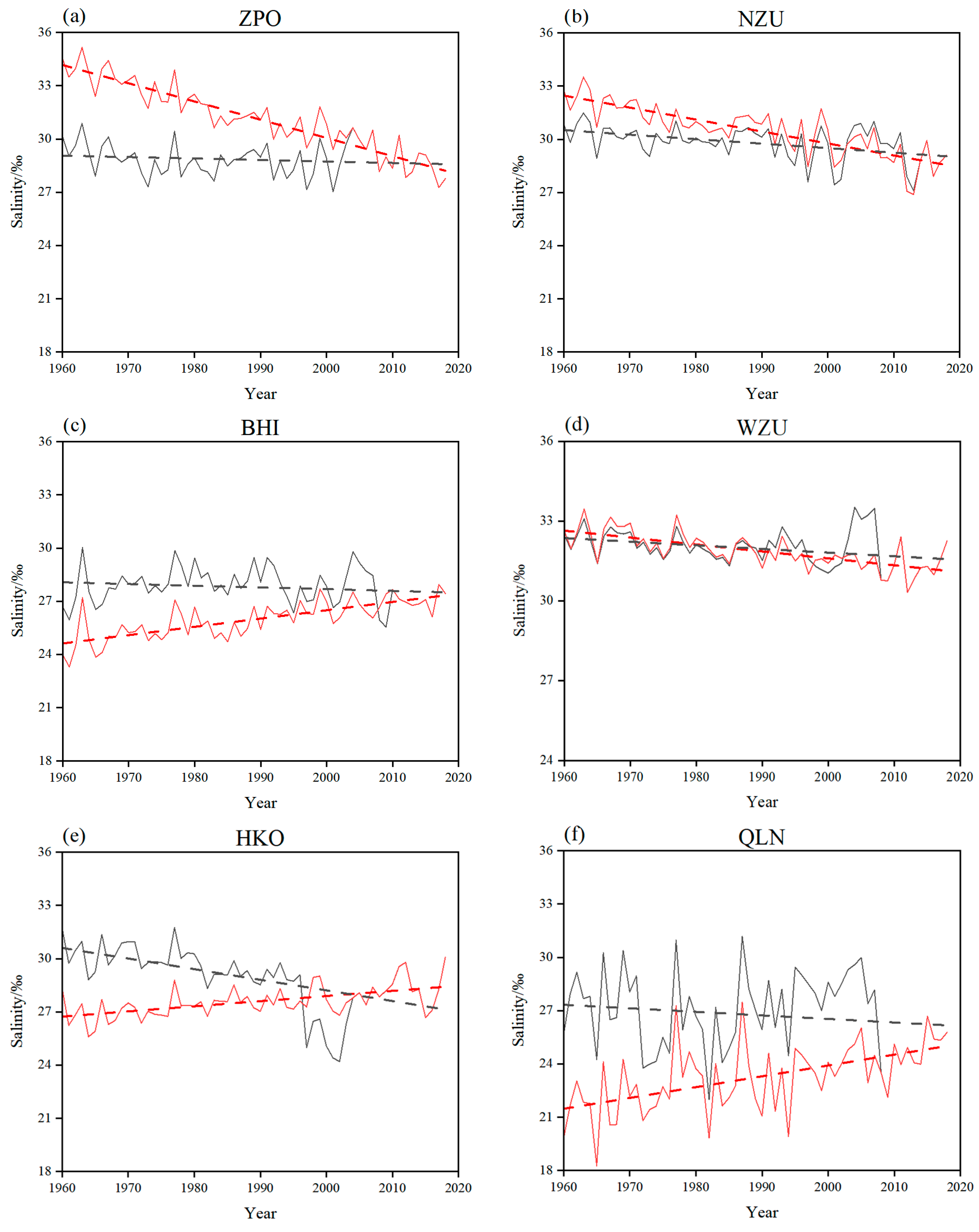
3.2. Analysis of Linear Trend Estimation of SSS Series before and after Homogenization Adjustment

It was found that there were significant differences in the annual mean values (Figure 3) and long-term trend rates (Table 4) before and after the homogeneity adjustment. Figure 3 presents the annual mean SSS series of the six coastal hydrological stations. The homogenized SSS values of the NZU, ZPO and WZH stations, represented by red solid lines, were greater than the raw SSS values, indicated by black solid lines. The homogenized annual mean SSS values of the remaining three coastal hydrological stations were significantly lower than raw values. This is related to the change in the salinity observation system in China (from manual observation to automatic observation, including instrument type, measurement frequency, measurement method and measurement depth). The instrument changes could potentially have had a substantial impact on the homogeneity of salinity data in the coastal regions.

In order to study the long-term trend of SSS data series before and after homogeneity adjustment, the linear trends in the raw and homogenized SSS during the period 1960–2018 were estimated via the least squares linear fitting method in this study. The results are shown in Figure 3 and Table 4. They show that all homogenized SSS series from the stations exhibited significant linear trends at the 95% confidence level. Both the raw and homogenized SSS series from the WZU, ZPO and NZU stations exhibited a trend of decreasing salinity. However, in general, the rate of increase was significantly higher in the homogenized SSS data than that in the raw data (e.g., there was no significant decreasing trend in the raw SSS data of the ZPO station). Thus, the freshening trends of seawater in the three stations were probably severely underestimated. Conversely, for the BHI, HKO and QLN stations, the homogenized SSS series revealed significant increasing salinity trends, in contrast to the decreasing trends observed in the raw series. In addition, these findings indicated a non-uniform spatial distribution of salinity long-term trends along the northern SCS coast. This may have been caused by complex geographical factors and regional climate influences. However, further investigation is required to enhance the understanding of the spatial pattern of the SSS changes.

3.3. Individual Case Analysis

As an illustration of the process of homogeneity identification and adjustment using the PMF method, we chose the long-term observational SSS series from the NZU and HKO stations.

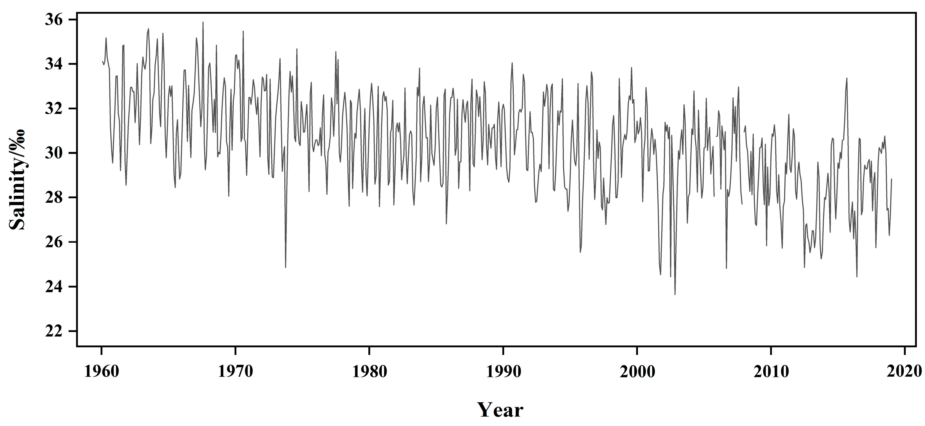
3.3.1. Detection and Adjustment of Monthly Mean SSS Series of NZU Station

Figure 4 displays the PMF test results of the monthly mean SSS series from the NZU station. There were three identified breakpoints in the SSS series, which are easily visible. Among them, July 1975 and April 2013 were recognized as Type-1 breakpoints, which were considered highly significant. The statistical test was conducted with a significance level of 95%. These breakpoints were statistically significant, even without the metadata support. Another one, in April 2003, was categorized as a Type-0 breakpoint, which refers to the changes documented in the metadata, although they had not yet been identified as a statistically significant Type-1 breakpoint. The accuracy of statistically identified breakpoints was validated using metadata and historical information. It was recorded in the metadata that an instrument change occurred in August 2003. These detected Type-0 breakpoints were considered to be real only when the metadata indicated the documented changes within 1 year before or after the date of the breakpoint detected with PMF. Thus, April 2003 was confirmed as a real breakpoint and identified as the documented breakpoint (Table 2). Then, the documented time (August 2003) replaced the PMF test time (April 2003) for adjustment. All of the adjustment results are shown in

Table 6. Inhomogeneity information of the monthly mean SSS from 1960 to 2018 at the NZU station.

Breakpoint Time	Detection Statistic	95% Confidence Interval	Adjusted Value (Unit: ‰)
July 1975	10.8321	31.5437~41.9330	1.77
April 2003	34.5494	31.3746~41.6887	0.80
April 2013	5.0618	29.9585~39.7163	−0.69

. The values ranged from −0.69 to 1.77‰. Figure 5 displays the homogenized monthly mean SSS series for the NZU station, indicating a notable decline in SSS.

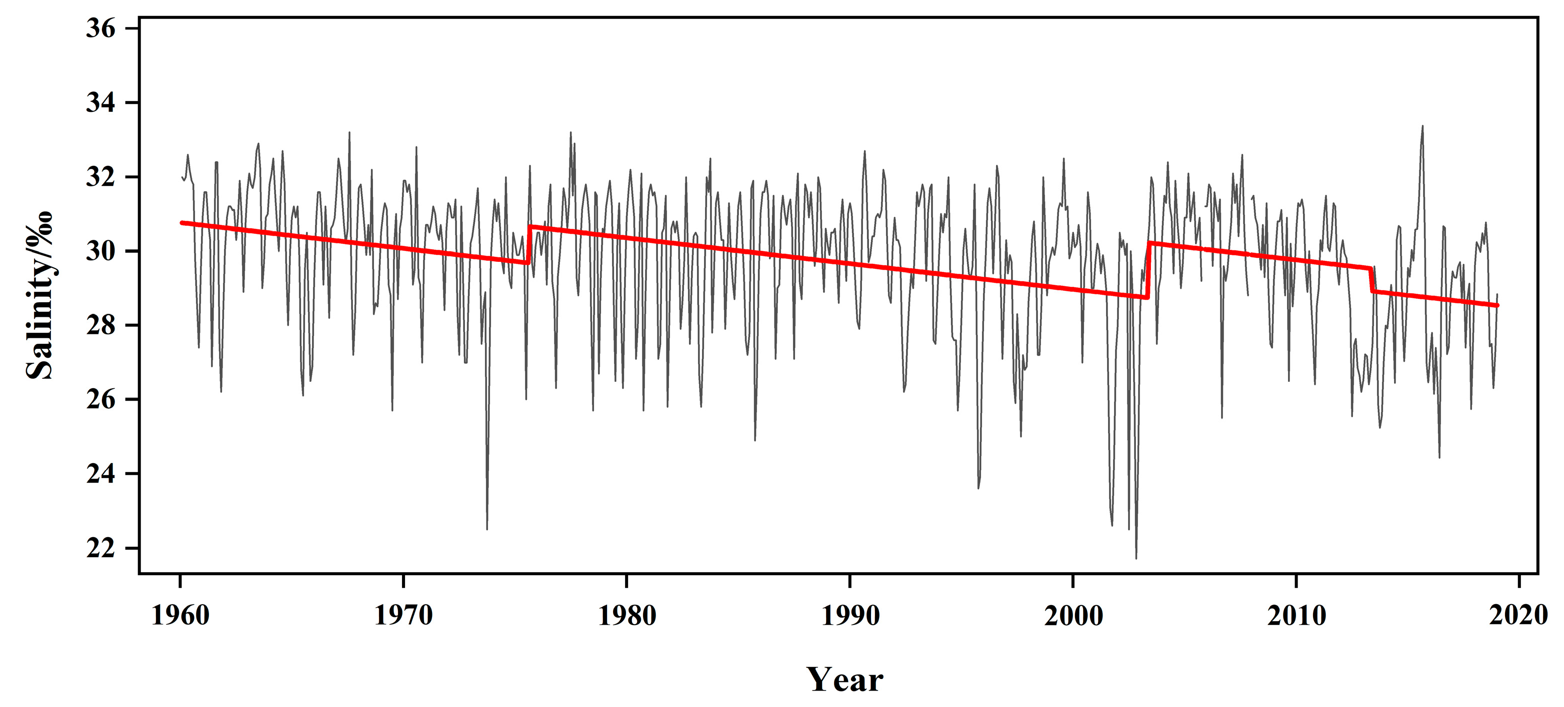
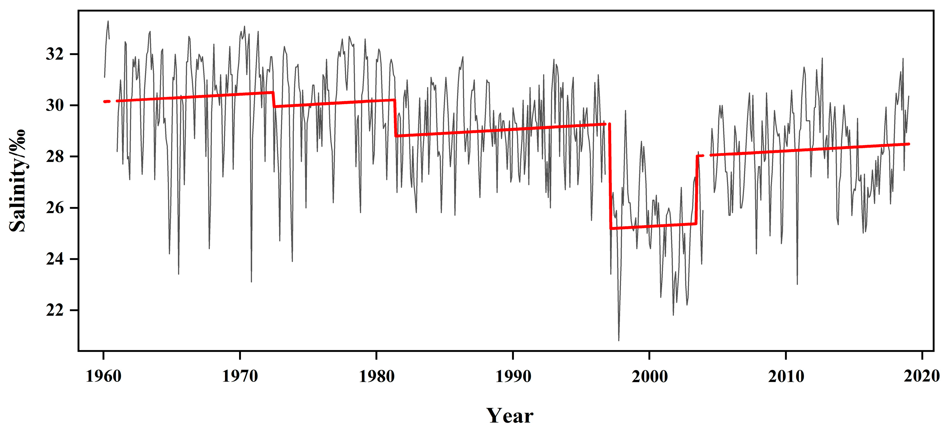
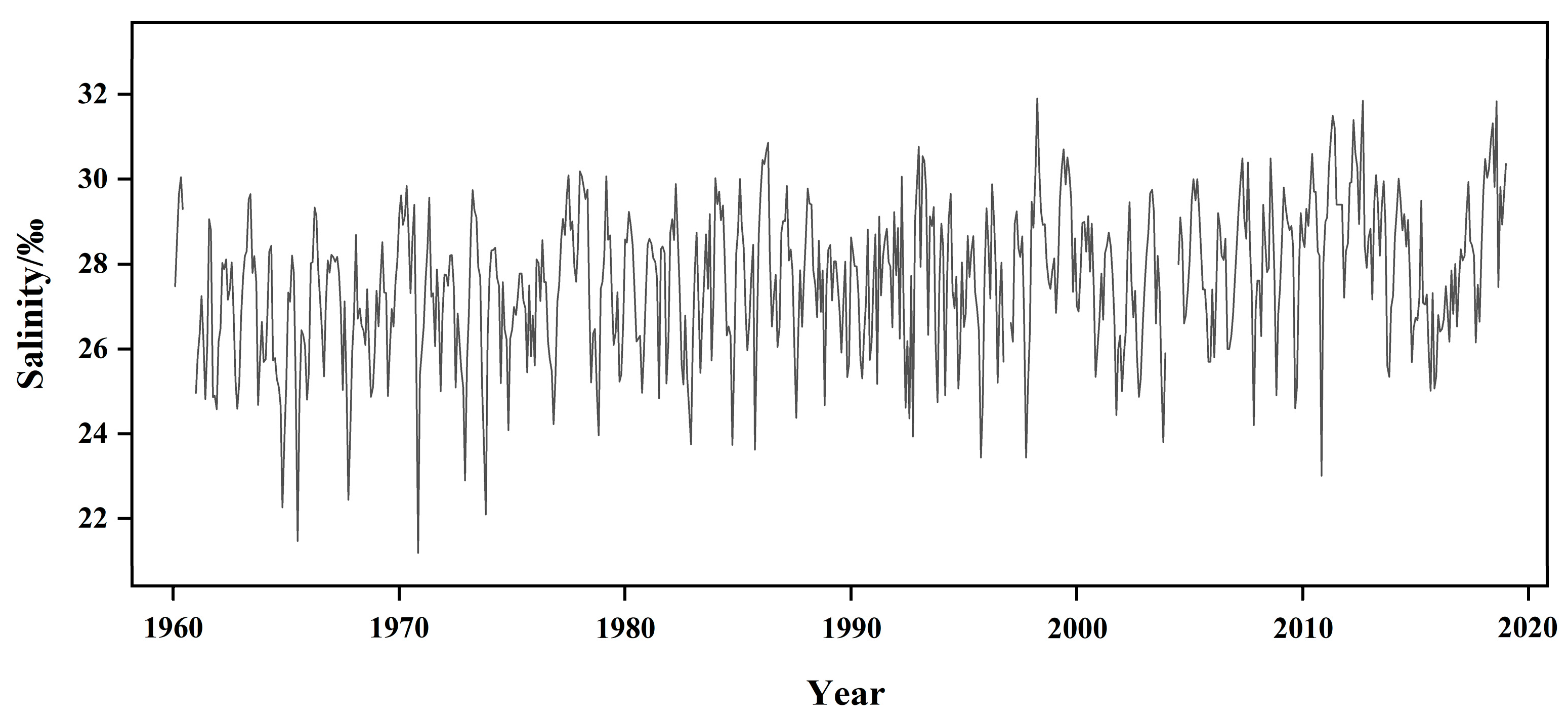
3.3.2. Detection and Adjustment of Monthly Mean SSS Series at the HKO Station

Figure 6 displays the PMF test results of the monthly mean SSS series from the HKO station. There were four breakpoints in the long-term SSS series. May 1972 was identified as a highly significant breakpoint, referred to as a Type-1 breakpoint. April 1981, January 1997 and May 2003 were identified as Type-0 breakpoints. It was recorded in the metadata that there were instrument changes in April 1982, January 1997 and October 2002 (see Table 3). These detected Type-0 breakpoints were considered to be real breakpoints only when the dates of the instrument changes were recorded in the metadata within 1 year before or after the date of the breakpoint detected using PMF and identified as documented breakpoints. The documented dates of changes were used to replace the test dates of change. The adjustment values are shown in

Table 7. Inhomogeneity information of the monthly mean SSS from 1960 to 2018 at the HKO station.

Breakpoint Time	Detection Statistic	95% Confidence Interval	Adjusted Value (Unit: ‰)
May 1972	34.2798	29.7167~39.5360	−0.57
April 1981	34.5999	29.9932~39.9183	−1.41
January 1997	34.3691	29.7938~39.6427	−4.10
May 2003	34.3319	29.7617~39.5983	2.65

, with values ranging from −4.10 to 2.65‰. As shown in the Figure 7, the seawater salinity shows a notable upward trend. It is worth noting that the salinity measurement point of the HKO station was located next to the tide gauge, surrounded by communities and ports; sewage from both affects the seawater salinity.

4. Discussion

Our primary objective was to detect and adjust the inhomogeneity and enhance the dependability of the monthly mean SSS data from the six regional hydrological stations spanning the period from 1960 to 2018. We also addressed the previously unexplored investigation of the spatial and temporal changes in SSS along the northern shore of the SCS based on the homogenized data. Due to the unique geographical environment of the southern coastal areas of the SCS, shallow water effects and terrestrial influences have led to complex changes in salinity in the region. The salinity of coastal waters is influenced by both large-scale environmental fields such as freshwater fluxes dominated by precipitation and evaporation, summer monsoon fields and local environmental conditions such as the upwelling of seawater, local ocean currents and temperature. Thus, we think that the greatest cause of regional disparities is the complex local environmental conditions.

Of the six stations investigated in this study, the SSS of the BHI, HKO and QLN stations exhibited a consistent upward trend in salinity from 1960 to 2018. The BHI station is located in the Beibu Gulf, Guangxi Province. The HKO and QLN stations are located on Hainan Island. These three stations are less affected by terrestrial climate conditions but are more susceptible to the impact of tropical cyclones, southwest monsoons and subtropical high pressures. As a result, there is a noticeable decrease in precipitation at these stations, as reported by Wu et al. [26] and Luo et al. [27]. These three stations are also affected by the SCS’s warm current, which originates from the warm surface seawater of the tropical western Pacific. Therefore, the SSS in this region has a notable response to El Niño events and precipitation changes. This is evident from the observed tendency of increasing salinity [28,29]. The ZPO and NZH stations are situated in the northeast of the SCS, where the ocean current conditions in this region are highly intricate. The seawater systems that flow into the northeast of the SCS consist of the Kuroshio branch, the SCS’s warm current and the coastal waters of the Fujian and Guangdong Providences. From 1960 to 2018, the SSS of the ZPO and NZH stations showed a clear desalination trend. This could be attributed to the rise in heavy summer rainfall, the increased influx of freshwater into the sea at the Pearl River Estuary and the reduction in coastal seawater transport caused by the intensification of Walker circulation in recent years [30,31,32,33]. The WZH station is located on Weizhou Island, which is located in the central part of the Beibu Gulf and influenced by South Asian tropical monsoons. Studies have indicated that since 1959, precipitation at Weizhou Island has fluctuated greatly and has shown a significant increasing trend in recent decades [34,35]. Moreover, the annual mean air temperature on Weizhou Island is 23.2 °C, and it is increasing at a rate of 0.10 °C per decade. However, from 1959 to 2014, there was a mere 0.6 °C rise in air temperature, indicating a relatively modest increase [36]. The SSS of the WZH station showed a relatively weak trend of seawater desalination compared to the ZPO and NZH stations, which is consistent with the local climate characteristics of Weizhou Island.

As the main content of this article is the homogenization detection and correction of salinity data in the SCS, and considering the length issue, we only discussed the regional differences in salinity trend changes from the perspectives of temperature, precipitation, ocean currents, etc., in this section, mainly citing previous research results as evidence. In the next stage of our research, we will collect more observational data on precipitation, temperature, evaporation and other factors to analyze the salinity changes at different sites. We will also utilize climate change signals such as the ENSO and Pacific Decadal Oscillation (PDO) [36,37,38] to analyze how large-scale circulation establishes a relationship with the local salinity change through local freshwater flux.

Although the sample size of coastal hydrological stations in this study was small, it has pioneering significance as it is the first attempt to detect and adjust SSS inhomogeneity along the northern coast of the SCS. Nevertheless, there were still certain deficiencies in this study. For instance, the scarcity of coastal hydrological stations in China posed a challenge in collecting nearby SSS series that may have served as a reference series. This is why we had to use the absolute method of PMF, which was not applicable to reference series but still presented a challenge in determining whether breakpoints were caused by non-climatic factors or climatic factors. Consequently, there may have been some uncertainties in the findings of the data homogenization. Accordingly, the detailed metadata were essential in verifying breakpoints. It is also necessary to employ multiple homogenization approaches (e.g., two-phase regression (TPR) procedures) in the future that can generate diverse homogenized results. Only the most consistent climate trends from these homogenized results are more closely linked to reality.

5. Conclusions

Long-term observational datasets from meteorological or hydrological stations are the fundamental basis of climate research. A homogenized long-term SSS record will significantly enhance our understanding of changes in the maritime environment. However, there is some inhomogeneity in the long-term series of raw SSS data along the coast of the northern SCS, which negatively impacts regional climate research. Therefore, this study utilized the PMFred algorithm together with metadata to homogenize and adjust the monthly mean SSS recorded at six ocean coastal hydrological stations. We studied the spatial and temporal variation characteristics of the homogenized SSS in the coastal regions and discussed the influence of regional climate change. The conclusions of this study are the following:

• All six SSS series were affected by non-climate factors. The main reason for the detected inconsistencies is the changes in instruments, particularly with the transition of the station system. Of the stations, BHI and WZU were the most affected by non-climate factors, with five breakpoints, while ZPO was the least with two breakpoints.
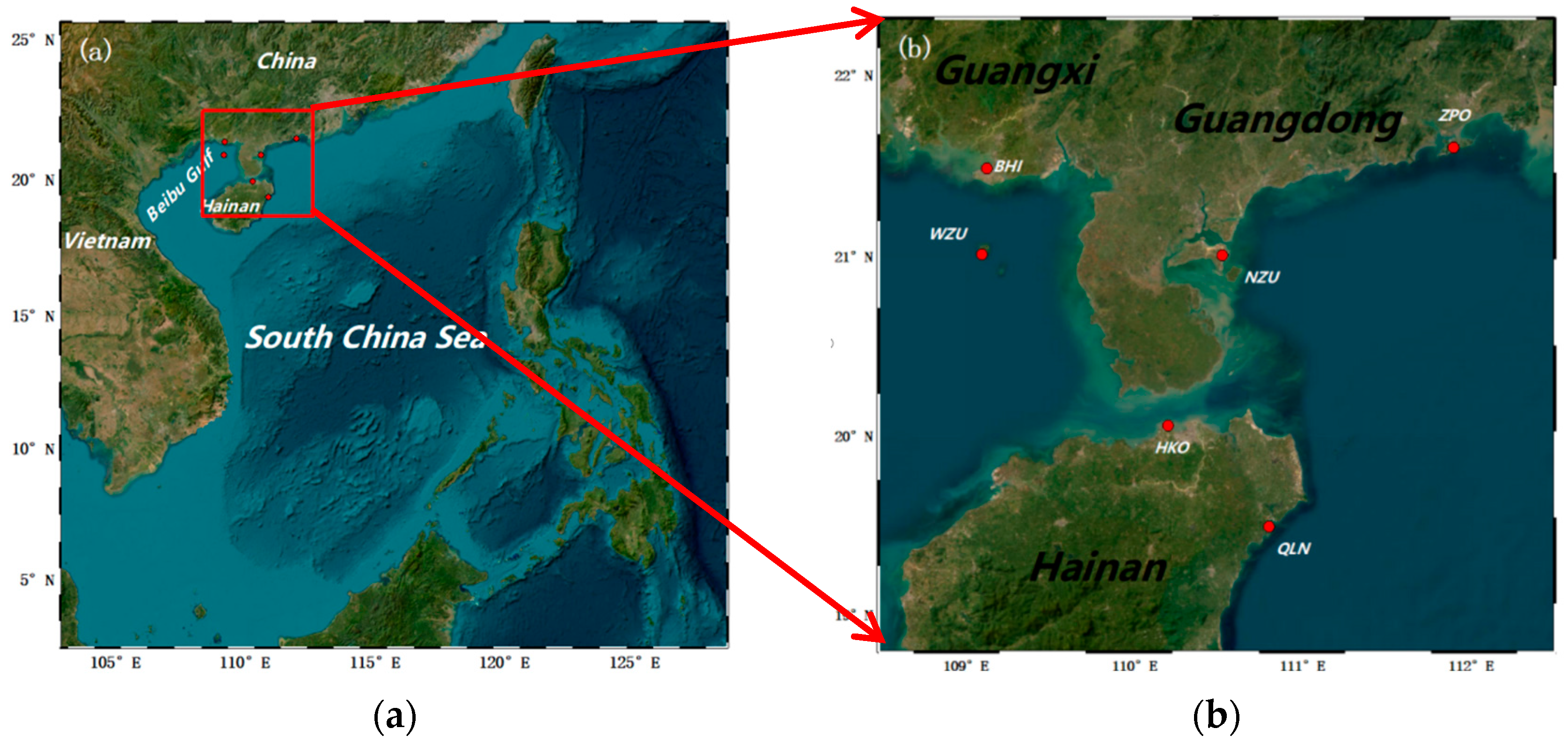
• The long-term fluctuations in homogenized SSS in the northern SCS showed notable regional variations. The coastal SSS measurements obtained from the BHI, HKO and QLN stations in Guangxi and Hainan Provinces exhibited a significant increase in salinity levels from 1960 to 2018. Nevertheless, the measurements obtained from the WZU, ZPO and NZH stations exhibited a distinct trend of desalination.

References

1. Cai, R.; Liu, K.; Tan, H. Impacts and risks of climate change on China’s coastal zones and seas and related adaptation. Chin. J. Popul. 2020, 30, 1–8. [Google Scholar]
2. Wang, F.; Li, X.; Tang, X.; Sun, X.; Zhang, J.; Yang, D.; Xu, L.; Zhang, H.; Yuan, H.; Wang, Y.; et al. The seas around China in a warming climate. Nat. Rev. Earth Environ. 2023, 4, 535–551. [Google Scholar] [CrossRef]
3. Röthig, T.; TrevathanTackett, S.M.; Voolstra, C.R.; Ross, C.; Chaffron, S.; Durack, P.J.; Warmuth, L.M.; Sweet, M. Human-induced salinity changes impact marine organisms and ecosystems. Glob. Chang. Biol. 2023, 29, 4731–4749. [Google Scholar] [CrossRef] [PubMed]
4. Vasiliev, I.; Karakitsios, V.; Bouloubassi, I.; Agiadi, K.; Kontakiotis, G.; Antonarakou, A.; Triantaphyllou, M.; Gogou, A.; Kafousia, N.; Rafélis, M.; et al. Large Sea Surface Temperature, Salinity, and Productivity-Preservation Changes Preceding the Onset of the Messinian Salinity Crisis in the Eastern Mediterranean Sea. Paleoceanogr. Paleoclimatol. 2019, 34, 182–202. [Google Scholar] [CrossRef]
5. Liu, F.; Zhang, H.; Ming, J.; Zheng, J.; Tian, D.; Chen, D. Importance of Precipitation on the Upper Ocean Salinity Response to Typhoon Kalmaegi (2014). Water 2020, 12, 614. [Google Scholar] [CrossRef]
6. Yang, Y.; Guo, Y.; Zeng, L.; Wang, Q. Eddy-induced sea surface salinity changes in the South China Sea. Front. Mar. Sci. 2023, 10, 1113752. [Google Scholar]
7. Ge, K.; Li, Y.; Lyu, Y.; Lin, P.; Cheng, L.; Wang, F. Surface Salinity Changes of the Tropical and Subtropical Oceans Since 1970 and Their Relationship With Surface Freshwater Fluxes. J. Geophys. Res. Ocean. 2023, 128, e2023JC020207. [Google Scholar] [CrossRef]
8. Ankrah, J.; Monteiro, A.; Madureira, H. Climate Variability, Coastal Livelihoods, and the Influence of Ocean Change on Fish Catch in the Coastal Savannah Zone of Ghana. Water 2024, 16, 1201. [Google Scholar] [CrossRef]
9. Wang, G.; Li, Y.; Hou, M.; Fan, W.; Liu, K.; Wang, H.; Gao, J.; Li, C. Homogeneity study of the sea surface temperature data over the South China Seas using PMT method. J. Trop. Meteorol. 2017, 33, 637–643, (In Chinese with English Abstract). [Google Scholar]
10. Li, Q.; Li, W. Construction of the gridded historic temperature dataset over China during the recent half century. Acta Meteorol. Sin. 2007, 02, 293–300, (In Chinese with English Abstract). [Google Scholar] [CrossRef]
11. Li, Q.; Liu, X.; Zhang, H.; Peterson, T.C.; Easterling, D.R. Detecting and adjusting temporal inhomogeneity in Chinese mean surface air temperature data. Adv. Atmos. Sci. 2004, 21, 260–268. [Google Scholar] [CrossRef]
12. Si, P.; Hao, L.; Luo, C.; Cao, X.; Liang, D. The Interpolation and Homogenization of Long-Term Temperature Time Series at Baoding Observation Station in Hebei Province. Adv. Clim. Chang. Res. 2017, 13, 41–51, (In Chinese with English Abstract). [Google Scholar]
13. Zhu, Y.; Cao, L.; Tang, G.; Zhou, Z. Homogenization of Surface Relative Humidity over China. Adv. Clim. Chang. Res. 2015, 11, 379–386, (In Chinese with English Abstract). [Google Scholar]
14. Li, Y.; Mu, L.; Wang, Q.; Ren, G.; You, Q. High-quality sea surface temperature measurements along coast of the Bohai and Yellow Seas in China and their long-term trends during 1960–2012. Int. J. Climatol. 2020, 40, 63–76. [Google Scholar] [CrossRef]
15. GB/T 14914-94; 1st ed. The Specification for Offshore Observation. China Standards Press: Beijing, China, 1994; pp. 1–100. (In Chinese)
16. GB/T 14914-2006; 1st ed. The Specification for Offshore Observation. China Standards Press: Beijing, China, 2006; pp. 1–83. (In Chinese)
17. Lü, H.; Xie, J.; Xu, J.; Chen, Z.; Liu, T.; Cai, X. Force and torque exerted by internal solitary waves in background parabolic current on cylindrical tendon leg by numerical simulation. Ocean Eng. 2016, 114, 250–258. [Google Scholar] [CrossRef]
18. Guan, M.; Cheng, Y.; Li, Q.; Wang, C.; Fang, X.; Yu, J. An Effective Method for Submarine Buried Pipeline Detection via Multi-Sensor Data Fusion. IEEE Access 2019, 7, 125300–125309. [Google Scholar] [CrossRef]
19. Guan, M.; Li, Q.; Zhu, J.; Wang, C.; Zhou, L.; Huang, C.; Ding, K. A method of establishing an instantaneous water level model for tide correction. Ocean Eng. 2019, 171, 324–331. [Google Scholar] [CrossRef]
20. Reeves, J.; Chen, J.; Wang, X.L.; Lund, R.; Lu, Q. A Review and Comparison of Changepoint Detection Techniques for Climate Data. J. Appl. Meteorol. Clim. 2007, 46, 900–915. [Google Scholar] [CrossRef]
21. Wang, X.L. Accounting for Autocorrelation in Detecting Mean Shifts in Climate Data Series Using the Penalized Maximal t or F Test. J. Appl. Meteorol. Climatol. 2008, 47, 2423–2444. [Google Scholar] [CrossRef]
22. Wang, X.L. Penalized Maximal F Test for Detecting Undocumented Mean Shift without Trend Change. J. Atmos. Ocean. Technol. 2008, 25, 368–384. [Google Scholar] [CrossRef]
23. ETCCDI Climate Change Indices. Available online: https://etccdi.pacificclimate.org/software.shtml (accessed on 1 September 2021).
24. Wang, X.L.; Chen, H.; Wu, Y.; Feng, Y.; Pu, Q. New Techniques for the Detection and Adjustment of Shifts in Daily Precipitation Data Series. J. Appl. Meteorol. Climatol. 2011, 49, 2416–2436. [Google Scholar] [CrossRef]
25. Sen, P. Estimated of the regression coefficient based on Kendall’s Tau. J. Am. Stat. Assoc. 1968, 39, 1379–1389. [Google Scholar] [CrossRef]
26. Wu, H.; Hu, D.; Xing, C.; Zhu, J. Characteristics of different types of precipitation and their influences on drought and flood over Hainan Island in summer. Torrential Rain Disasters 2021, 40, 558–563, (In Chinese with English Abstract). [Google Scholar]
27. Luo, J.; Wang, H.; Wang, A.; Fan, W.; Quan, M.; Zhang, J.; Wang, D. The precipitation changes in the coastal areas of China under the background of global climate warming. Mar. Sci. Bull. (Chin. Ed.) 2023, 42, 151–158, (In Chinese with English Abstract). [Google Scholar]
28. Guo, Z. Anomalies of sea surface temperature and salinity in Beibu Gulf during El Niño events. Trop. Oceanol. 1989, 8, 52–57, (In Chinese with English Abstract). [Google Scholar]
29. He, G.; Lu, W.; Liu, Y. An analysis on the periodicity of seawater salinity along the coast of Guangdong and Guangxi. Trop. Oceanol. 1993, 12, 25–30, (In Chinese with English Abstract). [Google Scholar]
30. Wang, L.; Li, Q.; Mao, X.; Bi, H.; Peng, Y. Interannual sea level variability in the Pearl River Estuary and its response to El Niño–Southern Oscillation. Glob. Planet. Chang. 2018, 162, 163–174. [Google Scholar] [CrossRef]
31. China Meteorological Administration. Blue Book on Climate Change of China 2019, 1st ed.; China Meteorological Administration: Beijing, China, 2019; pp. 1–80.
32. Pang, S.; Wang, X.; Liu, H.; Zhou, G.; Fan, K. Decadal Variability of the Barrier Layer and Forcing Mechanism in the Bay of Bengal. J. Geophys. Res. Ocean. 2019, 124, 5289–5307. [Google Scholar] [CrossRef]
33. Climate Change 2021: Summary for Policymakers. Available online: https://www.ipcc.ch/report/ar6/wg1/downloads/report/IPCC_AR6_WGI_SPM.pdf (accessed on 9 August 2021).
34. Liao, Q.; You, M.; Liu, X. Analysis of Climate Change Characteristics in the Near Sea of Weizhou Island over the Past 30 Years. J. Meteor. Res. Appl. 2012, 33, 140–141, (In Chinese with English Abstract). [Google Scholar]
35. Li, J.; Bai, A.; Cai, Q. Climate Change Characteristics of the Xisha Islands and Weizhou Island in China and the Comparison with the Coastal Land. Trop. Geo. 2018, 38, 72–81, (In Chinese with English Abstract). [Google Scholar]
36. Du, Y.; Zhang, Y.; Feng, M.; Wang, T.; Zhang, N.; Wijffels, S. Decadal trends of the upper ocean salinity in the tropical Indo-Pacific since mid-1990s. Sci. Rep. 2015, 5, 16050. [Google Scholar] [CrossRef] [PubMed]
37. Ramos, R.D.; Goodkin, N.F.; Siringan, F.P.; Hughen, K.A. Coral records of temperature and salinity in the tropical western Pacific reveal influence of the Pacific decadal oscillation since the late nineteenth century. Paleoceanogr. Paleocl. 2019, 34, 1344–1358. [Google Scholar] [CrossRef]
38. Hu, S.; Sprintall, J.; Guan, C.; Hu, D.; Wang, F.; Lu, X.; Li, S. Observed triple mode of salinity variability in the thermocline of tropical Pacific Ocean. J. Geophys. Res. Ocean. 2020, 125, e2020JC016210. [Google Scholar] [CrossRef]
Figure 1. Geographical maps of (a) the SCS and along the coast, with coastal hydrological stations indicated by small red rectangles; (b) coastal hydrological stations, with the point used for time series extraction (red dot).
Water 16 01895 g001
Figure 2. Flow chart of the inhomogeneity detection and adjustment processes.
Water 16 01895 g002
Figure 3. Annual mean SSS series (solid line) and its linear trend (dotted line) for the original series (in black color) and homogenized series (in red color) of the (a) ZPO, (b) NZU, (c) BHI, (d) WZU, (e) HKO and (f) QLN coastal hydrological stations.
Water 16 01895 g003
Figure 4. Monthly mean original SSS series (black line) and the estimated mean response along with the estimated mean shift (red line) of the NZU station.
Water 16 01895 g004
Figure 5. Monthly mean SSS series after adjustment of the NZU station from 1960 to 2018.
Water 16 01895 g005
Figure 6. Monthly mean original SSS series (black line) and the estimated mean response along with the estimated mean shift (red line) of the HKO station.
Water 16 01895 g006
Figure 7. Monthly mean SSS series after adjustment of the HKO station from 1960 to 2018.
Water 16 01895 g007