
Modeling of Future Streamflow Hazards in Interior Alaska River Systems and Implications for Applied Planning


Abstract
1. Introduction
2. Background
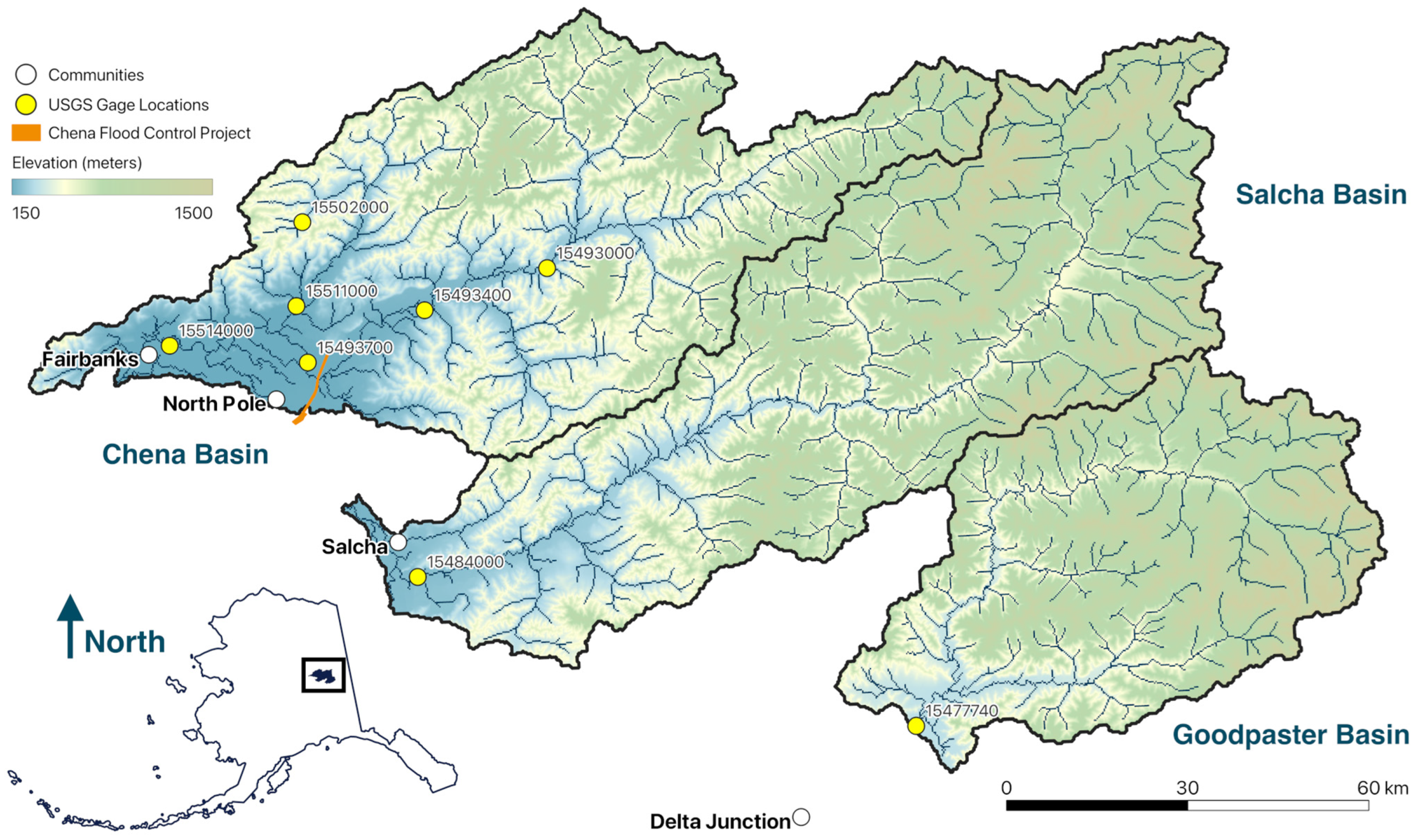
2.1. Study Area
2.2. Flood Control and Flood Events
2.3. Streamflow Gages
2.4. Discontinuous and Sporadic Permafrost
2.5. Hazard Assessment
3. Methods
3.1. Model Setup
3.2. Domain Setup
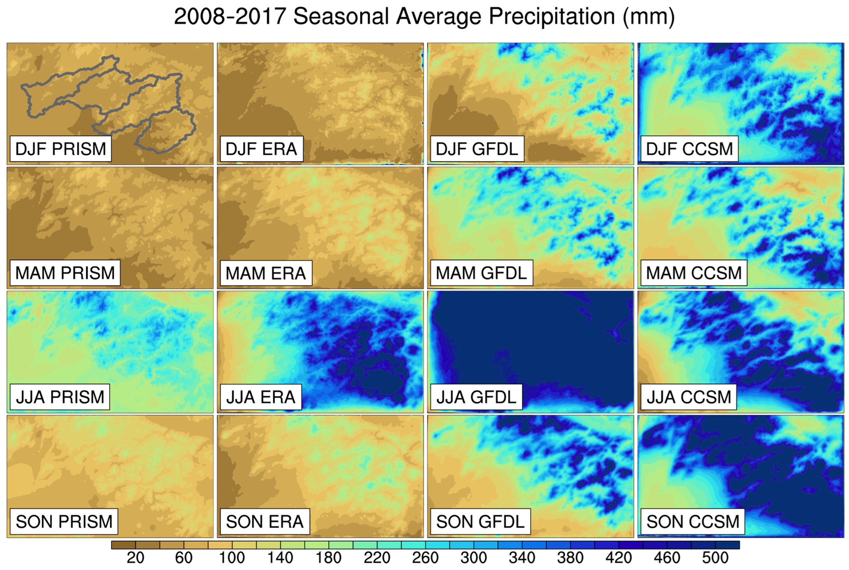
3.3. Forcing Data
3.4. Bias-Correction
3.5. Calibration
4. Results
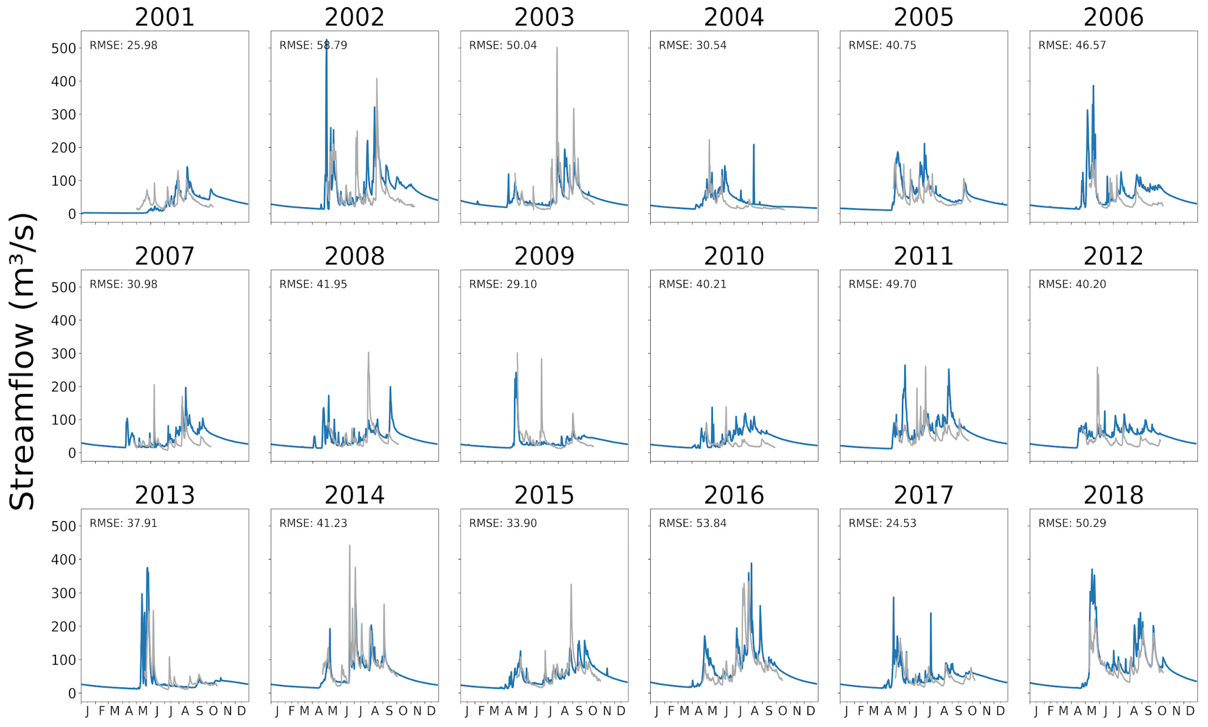
4.1. Calibration Results
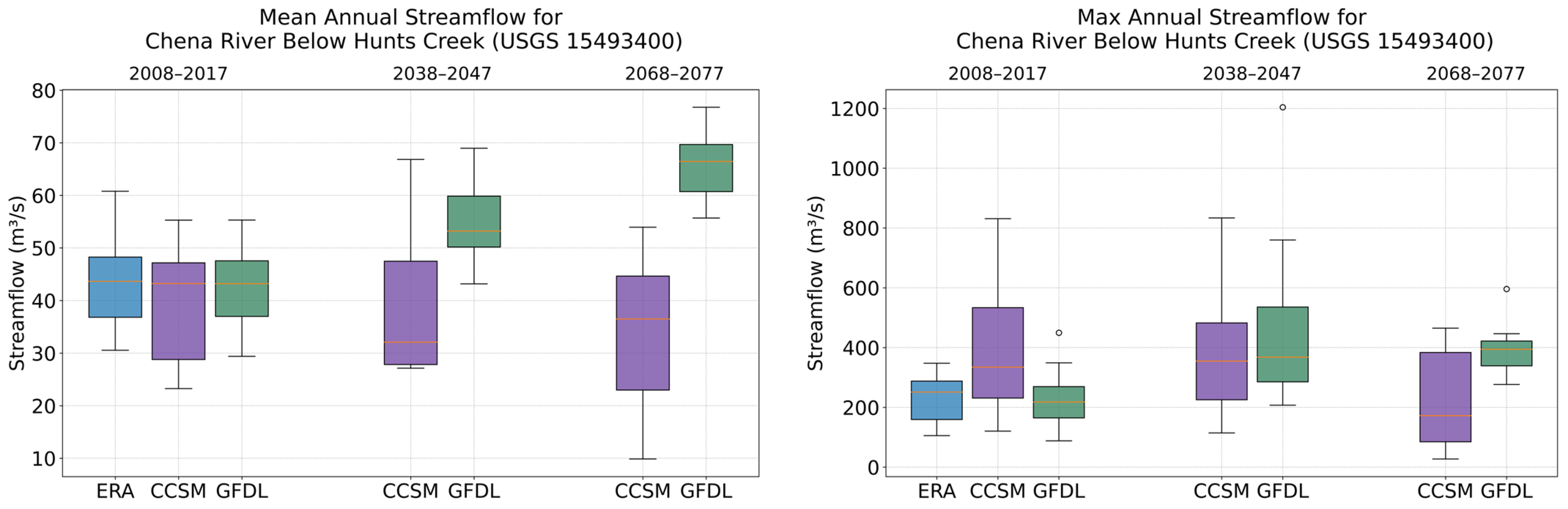
4.2. Model Divergence
4.3. Seasonality
4.4. Flood Control Implications
5. Discussion
5.1. Model Limitations
5.1.1. Stochasticity
5.1.2. WRF-Hydro Model Setup
5.1.3. Bias Variability and Uncertainty
5.2. Implications for Decision-Making
5.3. Future Improvements
6. Conclusions
Supplementary Materials
Author Contributions
Funding
Data Availability Statement
Acknowledgments
Conflicts of Interest
References
- Walvoord, M.A.; Kurylyk, B.L. Hydrologic Impacts of Thawing Permafrost—A Review. Vadose Zone J. 2016, 15, 1–20. [Google Scholar] [CrossRef]
- Douglas, T.A.; Turetsky, M.R.; Koven, C.D. Increased rainfall stimulates permafrost thaw across a variety of Interior Alaskan boreal ecosystems. npj Clim. Atmos. Sci. 2020, 3, 28. [Google Scholar] [CrossRef]
- Grosse, G.; Goetz, S.; McGuire, A.D.; Romanovsky, V.E.; Schuur, E.A.G. Changing permafrost in a warming world and feedbacks to the Earth system. Environ. Res. Lett. 2016, 11, 040201. [Google Scholar] [CrossRef]
- Jin, H.; Huang, Y.; Bense, V.F.; Ma, Q.; Marchenko, S.S.; Shepelev, V.V.; Hu, Y.; Liang, S.; Spektor, V.V.; Jin, X.; et al. Permafrost Degradation and Its Hydrogeological Impacts. Water 2022, 14, 372. [Google Scholar] [CrossRef]
- Estimating the Magnitude and Frequency of Peak Streamflows for Ungaged Sites on Streams in Alaska and Conterminous Basins in Canada. 2003. Available online: https://pubs.usgs.gov/wri/wri034188/ (accessed on 26 March 2024).
- Turnipseed, D.P.; Sauer, V.B. Discharge Measurements at Gaging Stations, Chap. A8, 87. In U.S. Geological Survey Techniques and Methods Book 3; U.S. Geological Survey: Reston, VA, USA, 2010. Available online: https://pubs.usgs.gov/publication/tm3A8 (accessed on 26 March 2024).
- Legleiter, C.J.; Kinzel, P.J. Inferring Surface Flow Velocities in Sediment-Laden Alaskan Rivers from Optical Image Sequences Acquired from a Helicopter. Remote Sens. 2020, 12, 1282. [Google Scholar] [CrossRef]
- Hodgkins, G.A. Streamflow changes in Alaska between the cool phase (1947–1976) and the warm phase (1977–2006) of the Pacific Decadal Oscillation: The influence of glaciers. Water Resour. Res. 2009, 45, 2008WR007575. [Google Scholar] [CrossRef]
- Liao, C.; Zhuang, Q. Quantifying the Role of Snowmelt in Stream Discharge in an Alaskan Watershed: An Analysis Using a Spatially Distributed Surface Hydrology Model. J. Geophys. Res. Earth Surf. 2017, 122, 2183–2195. [Google Scholar] [CrossRef]
- Bennett, K.E.; Cannon, A.J.; Hinzman, L. Historical trends and extremes in boreal Alaska river basins. J. Hydrol. 2015, 527, 590–607. [Google Scholar] [CrossRef]
- Bennett, K.E.; Schwenk, J.; Bachand, C.; Gasarch, E.; Stachelek, J.; Bolton, W.R.; Rowland, J.C. Recent streamflow trends across permafrost basins of North America. Front. Water 2023, 5, 1099660. [Google Scholar] [CrossRef]
- Cooper, M.G.; Zhou, T.; Bennett, K.E.; Bolton, W.R.; Coon, E.T.; Fleming, S.W.; Rowland, J.C.; Schwenk, J. Detecting Permafrost Active Layer Thickness Change from Nonlinear Baseflow Recession. Water Resour. Res. 2023, 59, e2022WR033154. [Google Scholar] [CrossRef]
- Lader, R.; Walsh, J.E.; Bhatt, U.S.; Bieniek, P.A. Projections of Twenty-First-Century climate extremes for Alaska via dynamical downscaling and quantile mapping. J. Appl. Meteorol. Climatol. 2017, 56, 2393–2409. [Google Scholar] [CrossRef]
- Gochis, D.; Barlage, M.; Cabell, R.; Dugger, A.; Fanfarillo, A.; FitzGerald, K.; McAllister, M.; McCreight, J.; RafieeiNasab, A.; Read, L.; et al. WRF-Hydro® v5.1.1; v5.1.1; Computer Software, Zenodo; UCAR: Boulder, CO, USA, 2020. [Google Scholar] [CrossRef]
- Walsh, J.E.; Bhatt, U.S.; Littell, J.S.; Leonawicz, M.; Lindgren, M.; Kurkowski, T.A.; Bieniek, P.A.; Thoman, R.; Gray, S.; Rupp, T.S. Downscaling of climate model output for Alaskan stakeholders. Environ. Model. Softw. 2018, 110, 38–51. [Google Scholar] [CrossRef]
- Bennett, K.E.; Cherry, J.E.; Balk, B.; Lindsey, S. Using MODIS estimates of fractional snow cover area to improve streamflow forecasts in interior Alaska. Hydrol. Earth Syst. Sci. 2019, 23, 2439–2459. [Google Scholar] [CrossRef]
- Walvoord, M.A.; Striegl, R.G. Increased groundwater to stream discharge from permafrost thawing in the Yukon River basin: Potential impacts on lateral export of carbon and nitrogen. Geophys. Res. Lett. 2007, 34, 2007GL030216. [Google Scholar] [CrossRef]
- Young, B.; Yarie, J.; Verbyla, D.; Huettmann, F.; Herrick, K.; Chapin, F.S. Modeling and mapping forest diversity in the boreal forest of interior Alaska. Landsc. Ecol. 2017, 32, 397–413. [Google Scholar] [CrossRef]
- Mann, D.H.; Rupp, T.S.; Olson, M.A.; Duffy, P.A. Is Alaska’s Boreal Forest Now Crossing a Major Ecological Threshold? Arct. Antarct. Alp. Res. 2012, 44, 319–331. [Google Scholar] [CrossRef]
- Wendler, G.; Shulski, M. A Century of Climate Change for Fairbanks, Alaska. ARCTIC 2009, 62, 295–300. [Google Scholar] [CrossRef]
- Ballinger, T.J.; Bhatt, U.S.; Bieniek, P.A.; Brettschneider, B.; Lader, R.T.; Littell, J.S.; Thoman, R.L.; Waigl, C.F.; Walsh, J.E.; Webster, M.A. Alaska Terrestrial and Marine Climate Trends, 1957–2021. J. Clim. 2023, 36, 4375–4391. [Google Scholar] [CrossRef]
- USDA Natural Resources Conservation Service. (n.d.). Upper Chena, AK (952) Precipitation Accumulation. Available online: https://nwcc-apps.sc.egov.usda.gov/awdb/site-plots/POR/PREC/AK/Upper%20Chena.html (accessed on 23 March 2024).
- U.S. Census Bureau. (n.d.). QuickFacts: Fairbanks North Star Borough, Alaska. Available online: https://www.census.gov/quickfacts/fact/table/fairbanksnorthstarboroughalaska/POP010220 (accessed on 23 March 2024).
- U.S. Army Corps of Engineers. Moose Creek Dam Modification Study Chena River Lakes Flood Control Project North Pole, Alaska [Environmental Assessment]. 2018. Available online: https://www.poa.usace.army.mil/Portals/34/docs/civilworks/publicreview/MCDSMREA.pdf (accessed on 10 December 2023).
- USGS. 5 Meter Alaska Digital Elevation Models (DEMs)—USGS National Map 3DEP Downloadable Data Collection: U.S. Geological Survey. 2022. Available online: https://www.sciencebase.gov/catalog/item/5641fe98e4b0831b7d62e758 (accessed on 17 August 2023).
- Childers, J.M.; Meckel, J.P.; Anderson, G.S. Floods of August 1967 in East-Central Alaska. August. 1972. Available online: https://pubs.usgs.gov/wsp/1880a/report.pdf (accessed on 3 September 2023).
- Bureau of Labor and Statistics. (n.d.). CPI Inflation Calculator. Available online: https://data.bls.gov/cgi-bin/cpicalc.pl (accessed on 10 November 2023).
- Flood Control Act of 1968, Pub. L. No. 90–483, 33 U.S.C. 739. 1968. Available online: http://govinfo.gov/content/pkg/STATUTE-82/pdf/STA (accessed on 2 March 2024).
- U.S. Army Corps of Engineers. Overview of Tanana River Monitoring and Research Studies Near Fairbanks. Alaska. 1984. Available online: https://archive.org/details/DTIC_ADA167790 (accessed on 6 November 2023).
- Vuyovich, C.M.; Daly, S.F.; The Chena River Watershed Hydrology Model (ERDC/CRREL TR-12-1). CRREL 2012. Available online: https://apps.dtic.mil/sti/citations/tr/ADA572119 (accessed on 10 December 2023).
- Napolitan, Rachel. General Visits Northernmost USACE-Run Flood Control Project. U.S. Army Corps of Engineers. Available online: https://www.usace.army.mil/Media/News-Archive/Story-Article-View/Article/2544915/general-visits-northernmost-usace-run-flood-control-project/ (accessed on 10 December 2023).
- Glass, R.L.; Lily, M.R.; Meyer, D.F. Ground-Water Levels in an Alluvial Plain Between the Tanana and Chena Rivers Near Fairbanks, Alaska. USGS. 1996. Available online: https://dec.alaska.gov/media/15613/gw-levels-alluvial-plain-tanana-chena.pdf (accessed on 8 January 2024).
- USACE. (n.d.). Innovation Leads to Productive Season for Safety Upgrade at Moose Creek Dam. Available online: https://www.poa.usace.army.mil/Media/News-Releases/Article/3583092/innovation-leads-to-productive-season-for-safety-upgrade-at-moose-creek-dam/ (accessed on 8 January 2024).
- U.S. Army Corps of Engineers, Fairbanks North Star Borough. Portion of Moose Creek Dam Crest Closed to Public at Chena Project > Alaska District > News Releases. U.S. Army Corps of Engineers Alaska District. Available online: https://www.poa.usace.army.mil/Media/News-Releases/Article/3444987/joint-news-release-portion-of-moose-creek-dam-crest-closed-to-public-at-chena-p/ (accessed on 24 March 2024).
- U.S. Army Corps of Engineers. Chena River Lakes Flood Control Project and Tanana River Levee. 2019. Available online: https://www.poa.usace.army.mil/Portals/34/docs/operations/EFC/2019ChenaTananaOverview.pdf (accessed on 24 March 2024).
- Rozell, N. Fixing the Fatal Flaw of Fairbanks. Geophysical Institute. Available online: https://www.gi.alaska.edu/alaska-science-forum/fixing-fatal-flaw-fairbanks (accessed on 24 March 2024).
- Pawłowski, B. Ice Jams: Causes and Effects. In Encyclopedia of Water, 1st ed.; Maurice, P., Ed.; Wiley: Hoboken, NJ, USA, 2019; pp. 1–9. [Google Scholar] [CrossRef]
- Napolitan, Rachel. Ice Jams Trigger Operation of the Moose Creek Dam on Chena River. U.S. Army Corps of Engineers. Available online: https://www.usace.army.mil/Media/News-Archive/Story-Article-View/Article/2183041/ice-jams-trigger-operation-of-the-moose-creek-dam-on-chena-river/ (accessed on 10 December 2023).
- FNSB Emergency Management. Multi-Jurisdictional Hazard Mitigation Plan. Fairbanks North Star Borough. 2021. Available online: https://www.fnsb.gov/DocumentCenter/View/8530/FNSB_MJHMP_Final_Sept2021 (accessed on 10 December 2023).
- Bohman, A.; Eshleman, C. Tanana, Salcha Rivers Flood Interior Alaska. Fairbanks Daily Newsminer. Available online: https://web.archive.org/web/20080811164339/http://www.newsminer.com/news/2008/jul/31/tanana-salcha-rivers-flood-interior-alaska/ (accessed on 25 March 2024).
- HDR, Inc. Alaska State Rail Plan—Final. 2016. Available online: https://dot.alaska.gov/railplan/docs/Rail-Plan-Final-draft.pdf (accessed on 25 March 2024).
- Ellis, T. (Director). Tanana River Bridge Levee Helped Deflect Breakup Floodwaters, Residents Say. KUAC. Available online: https://fm.kuac.org/local-news/2013-06-04/tanana-river-bridge-levee-helped-deflect-breakup-floodwaters-residents-say (accessed on 25 March 2024).
- USGS. (n.d.). Current Conditions for Alaska Streamflow. Available online: https://waterdata.usgs.gov/ak/nwis/current/?type=flow (accessed on 4 February 2024).
- Follansbee, R. A History of the Water Resources Branch, U.S. Geological Survey, Volume I; from Predecessor Surveys to 30 June 1919 [Report]; USGS Publications Warehouse: Reston, VA, USA, 1994. [Google Scholar] [CrossRef]
- USGS. Chena R BL Hunts C NR Two Rivers AK. USGS Water Data for the Nation. 2023. Available online: https://waterdata.usgs.gov/monitoring-location/15493400/ (accessed on 3 November 2023).
- Chapter 29: Alaska. In Fifth National Climate Assessment; U.S. Global Change Research Program: Reston, VA, USA, 2023. [CrossRef]
- Minsley, B.J.; Pastick, N.J.; James, S.R.; Brown, D.R.N.; Wylie, B.K.; Kass, M.A.; Romanovsky, V.E. Rapid and Gradual Permafrost Thaw: A Tale of Two Sites. Geophys. Res. Lett. 2022, 49, e2022GL100285. [Google Scholar] [CrossRef]
- Obu, J.; Westermann, S.; Bartsch, A.; Berdnikov, N.; Christiansen, H.H.; Dashtseren, A.; Delaloye, R.; Elberling, B.; Etzelmüller, B.; Kholodov, A.; et al. Northern Hemisphere permafrost map based on TTOP modelling for 2000–2016 at 1 km2 scale. Earth-Sci. Rev. 2019, 193, 299–316. [Google Scholar] [CrossRef]
- Smith, S.L.; O’Neill, H.B.; Isaksen, K.; Noetzli, J.; Romanovsky, V.E. The changing thermal state of permafrost. Nat. Rev. Earth Environ. 2022, 3, 10–23. [Google Scholar] [CrossRef]
- Deemy, J.B.; Takagi, K.K.; McLachlan, R.L.; Rasmussen, T.C.; Wright, S.G.; Tyler, K.N.; Garner, M.G. Hydrology, geomorphology, and soils: An overview. In Fundamentals of Tropical Freshwater Wetlands; Elsevier: Amsterdam, The Netherlands, 2022; pp. 43–86. [Google Scholar] [CrossRef]
- Osetinsky-Tzidaki, I.; Fredj, E. The 50- and 100-year Exceedance Probabilities as New and Convenient Statistics for a Frequency Analysis of Extreme Events: An Example of Extreme Precipitation in Israel. Water 2022, 15, 44. [Google Scholar] [CrossRef]
- Holmes, R.R., Jr.; Dinicola, K. 100-Year Flood–It’s All about Chance; Report 106; General Information Product; USGS Publications Warehouse: Reston, VA, USA, 2010. [Google Scholar] [CrossRef]
- Bird, L.J.; Bodeker, G.E.; Clem, K.R. Sensitivity of extreme precipitation to climate change inferred using artificial intelligence shows high spatial variability. Commun. Earth Environ. 2023, 4, 469. [Google Scholar] [CrossRef]
- Vogel, R.M.; Yaindl, C.; Walter, M. Nonstationarity: Flood Magnification and Recurrence Reduction Factors in the United States1: Nonstationarity: Flood Magnification and Recurrence Reduction Factors in the United States. JAWRA J. Am. Water Resour. Assoc. 2011, 47, 464–474. [Google Scholar] [CrossRef]
- IPCC. Managing the Risks of Extreme Events and Disasters to Advance Climate Change Adaptation. A Special Report of Working Groups I and II of the Intergovernmental Panel on Climate Change. In Special Report of the Intergovernmental Panel on Climate Change; Field, C.B., Barros, V., Stocker, T.F., Dahe, Q., Dokken, D.J., Ebi, K.L., Mastrandrea, M.D., Mach, K.J., Plattner, G.-K., Allen, S.K., et al., Eds.; Cambridge University Press: Cambridge, UK, 2012; Available online: https://www.ipcc.ch/report/managing-the-risks-of-extreme-events-and-disasters-to-advance-climate-change-adaptation/ (accessed on 25 March 2024).
- FEMA. 2023 National Household Survey on Disaster Preparedness. 2023. Available online: https://fema-community-files.s3.amazonaws.com/2023-National-Household-Survey.pdf (accessed on 8 January 2024).
- Lechowska, E. What determines flood risk perception? A review of factors of flood risk perception and relations between its basic elements. Nat. Hazards 2018, 94, 1341–1366. [Google Scholar] [CrossRef]
- Research Applications Laboratory. (n.d.). WRF-Hydro® Modeling System. Available online: https://ral.ucar.edu/projects/wrf_hydro (accessed on 23 March 2024).
- Gochis, D.J.; Barlage, M.; Cabell, R.; Casali, M.; Dugger, A.; FitzGerald, K.; McAllister, M.; McCreight, J.; RafieeiNasab, A.; Read, L.; et al. The NCAR WRF-Hydro Modeling System Technical Description, Version 5.1.1; National Center for Atmospheric Research: Boulder, CO, USA, 2020; Available online: https://ral.ucar.edu/sites/default/files/public/WRFHydroV511TechnicalDescription.pdf (accessed on 23 March 2024).
- NOAA. National Water Model: Improving NOAA’s Water Prediction Services. 2016. August. Available online: https://water.noaa.gov/assets/styles/public/images/wrn-national-water-model.pdf (accessed on 3 September 2023).
- Farrar, M. Upgrade of National Water Model on NCEP’s WCOSS System and Its Post-processing Application on the Integrated Dissemination Platform (IDP). 2023. Available online: https://www.weather.gov/media/notification/pdf_2023_24/scn23-76_national_water_model_v3.0_aab.pdf (accessed on 21 November 2023).
- Bieniek, P.A.; Bhatt, U.S.; Walsh, J.E.; Rupp, T.S.; Zhang, J.; Krieger, J.R.; Lader, R. Dynamical downscaling of ERA-interim temperature and precipitation for Alaska. J. Appl. Meteorol. Climatol. 2016, 55, 635–654. [Google Scholar] [CrossRef]
- Cannon, A.J.; Sobie, S.R.; Murdock, T.Q. Bias correction of GCM precipitation by quantile mapping: How well do methods preserve changes in quantiles and extremes? J. Clim. 2015, 28, 6938–6959. [Google Scholar] [CrossRef]
- ECMWF. (n.d.). ECMWF Datasets (ERA-Interim). Available online: https://www.ecmwf.int/en/forecasts/dataset/ecmwf-reanalysis-interim (accessed on 6 December 2023).
- Caswell, T.A.; Andrade, E.S.; de Lee, A.; Droettboom, M.; Hoffmann, T.; Klymak, J.; Hunter, J.; Firing, E.; Stansby, D.; Varoquaux, N.; et al. Matplotlib/Matplotlib: REL: v3.7.2; v3.7.2; Computer Software Zenodo; UCAR: Boulder, CO, USA, 2023. [Google Scholar] [CrossRef]
- Harris, C.R.; Millman, K.J.; Walt, S.J. van der, Gommers, R.; Virtanen, P.; Cournapeau, D.; Wieser, E.; Taylor, J.; Berg, S.; Smith, N.J.; et al. Array programming with NumPy. Nature 2020, 585, 357–362. [Google Scholar] [CrossRef] [PubMed]
- The Pandas Development Team. Pandas-Dev/Pandas: Pandas, v2.0.3; Computer Software Zenodo; UCAR: Boulder, CO, USA, 2023. [Google Scholar] [CrossRef]
- Hoyer, S.; Roos, M.; Joseph, H.; Magin, J.; Cherian, D.; Fitzgerald, C.; Hauser, M.; Fujii, K.; Maussion, F.; Imperiale, G.; et al. Xarray, v2023.06.0. Computer Software Zenodo. UCAR: Boulder, CO, USA, 2023. [CrossRef]
- Skamarock, W.; Klemp, J.; Dudhia, J.; Gill, D.; Barker, D.; Wang, W.; Huang, X.-Y.; Duda, M. A Description of the Advanced Research WRF Version 3; (p. 1002 KB) [Application/pdf]; UCAR/NCAR: Boulder, CO, USA, 2008. [Google Scholar] [CrossRef]
- Taylor, K.E.; Stouffer, R.J.; Meehl, G.A. An Overview of CMIP5 and the Experiment Design. Bull. Am. Meteorol. Soc. 2012, 93, 485–498. [Google Scholar] [CrossRef]
- Gent, P.R.; Danabasoglu, G.; Donner, L.J.; Holland, M.M.; Hunke, E.C.; Jayne, S.R.; Lawrence, D.M.; Neale, R.B.; Rasch, P.J.; Vertenstein, M.; et al. The Community Climate System Model Version 4. J. Clim. 2011, 24, 4973–4991. [Google Scholar] [CrossRef]
- Donner, L.J.; Wyman, B.L.; Hemler, R.S.; Horowitz, L.W.; Ming, Y.; Zhao, M.; Golaz, J.-C.; Ginoux, P.; Lin, S.-J.; Schwarzkopf, M.D.; et al. The Dynamical Core, Physical Parameterizations, and Basic Simulation Characteristics of the Atmospheric Component AM3 of the GFDL Global Coupled Model CM3. J. Clim. 2011, 24, 3484–3519. [Google Scholar] [CrossRef]
- van Vuuren, D.P.; Edmonds, J.; Kainuma, M.; Riahi, K.; Thomson, A.; Hibbard, K.; Hurtt, G.C.; Kram, T.; Krey, V.; Lamarque, J.F.; et al. The representative concentration pathways: An overview. Clim. Chang. 2011, 109, 5–31. [Google Scholar] [CrossRef]
- Markon, C.; Gray, S.; Berman, M.; Eerkes-Medrano, L.; Hennessy, T.; Huntington, H.P.; Littell, J.; McCammon, M.; Thoman, R.; Trainor, S.F. Chapter 26: Alaska. Impacts, Risks, and Adaptation in the United States. In The Fourth National Climate Assessment, Volume II; U.S. Global Change Research Program: Reston, VA, USA, 2018. [Google Scholar] [CrossRef]
- Peters, G.P.; Andrew, R.M.; Boden, T.; Canadell, J.G.; Ciais, P.; Le Quéré, C.; Marland, G.; Raupach, M.R.; Wilson, C. The challenge to keep global warming below 2 °C. Nat. Clim. Chang. 2013, 3, 4–6. [Google Scholar] [CrossRef]
- Sampson, K.; Gochis, D. WRF Hydro GIS Pre-Processing Tools, Version 5.1.1 Documentation. 2020. Available online: https://ral.ucar.edu/projects/wrf_hydro/pre-processing-tools (accessed on 6 November 2023).
- Aquatic Ecosystem Vulnerability to Fire and Climate Change in Alaskan Boreal Forests. (n.d.). Available online: https://serdp-estcp.mil/projects/details/1454fd5a-c908-4a7a-8a39-2c9dfa18519d/rc18-1108-project-overview (accessed on 4 February 2024).
- PRISM Climate Group at Oregon State University. United States Average Annual Total Precipitation, 1991–2020 (4 km; BIL) [dataset]. 2022. Available online: https://prism.oregonstate.edu (accessed on 22 April 2024).
- Logan, T.; Aoun, A.; Bourgault, P.; Dupuis, É.; Huard, D.; Lavoie, J.; Rondeau-Genesse, G.; Smith, T.J.; Alegre, R.; Barnes, C.; et al. Ouranosinc/xclim: V0.39.0; v0.39.0; Computer Software Zenodo; UCAR: Boulder, CO, USA, 2022. [Google Scholar] [CrossRef]
- RafieeiNasab, A.; Dugger, A.; FitzGerald, K.; Gochis, D.; Enzminger, T.; Mazrooei, A.; McAllister, M.; Srivastava, I.; Cabell, R.; Saylor, P.; et al. Overview of WRF-Hydro Model Calibration General Strategy Optimization. Available online: https://ral.ucar.edu/sites/default/files/public/projects/wrf-hydro/training-materials/Overview_of_Model_Calibration_Arezoo.pdf (accessed on 8 February 2024).
- Mauricio Zambrano-Bigiarini. hydroGOF: Goodness-of-Fit Functions for Comparison of Simulated and Observed Hydrological Time Series; Version: 0.4-0; 2020; Available online: https://zenodo.org/records/3707013 (accessed on 3 July 2024). [CrossRef]
- Mizukami, N.; Rakovec, O.; Newman, A.J.; Clark, M.P.; Wood, A.W.; Gupta, H.V.; Kumar, R. On the choice of calibration metrics for “high-flow” estimation using hydrologic models. Hydrol. Earth Syst. Sci. 2019, 23, 2601–2614. [Google Scholar] [CrossRef]
- Knoben, W.J.M.; Freer, J.E.; Woods, R.A. Technical note: Inherent benchmark or not? Comparing Nash-Sutcliffe and Kling-Gupta efficiency scores. Hydrol. Earth Syst. Sci. 2019, 23, 4323–4331. [Google Scholar] [CrossRef]
- Frantzeskaki, N.; McPhearson, T.; Collier, M.J.; Kendal, D.; Bulkeley, H.; Dumitru, A.; Walsh, C.; Noble, K.; Van Wyk, E.; Ordóñez, C.; et al. Nature-Based Solutions for Urban Climate Change Adaptation: Linking Science, Policy, and Practice Communities for Evidence-Based Decision-Making. BioScience 2019, 69, 455–466. [Google Scholar] [CrossRef]
- Stakhiv, E.Z. The centrality of engineering codes and risk-based design standards in climate adaptation strategies. Water Policy 2021, 23 (Suppl. S1), 106–127. [Google Scholar] [CrossRef]
- Chapter 31: Adaptation. In Fifth National Climate Assessment; U.S. Global Change Research Program: Reston, VA, USA, 2023. [CrossRef]
- Littell, J.; McAfee, S.; Hayward, G. Alaska Snowpack Response to Climate Change: Statewide Snowfall Equivalent and Snowpack Water Scenarios. Water 2018, 10, 668. [Google Scholar] [CrossRef]
- Druckenmiller, M.L.; Thoman, R.L.; Moon, T.A. NOAA Arctic Report Card 2022: Executive Summary; NOAA: Washington, DC, USA, 2022. [Google Scholar] [CrossRef]
- Walker, W.E.; Harremoes, P.; Rotmans, J.; Van Der Sluijs, J.P.; Van Asselt, M.B.A.; Janssen, P.; Krayer Von Krauss, M.P. Defining Uncertainty. Integr. Assess. 2003, 4, 5–17. [Google Scholar] [CrossRef]
- Guan, T.; Liu, Y.; Sun, Z.; Zhang, J.; Chen, H.; Wang, G.; Jin, J.; Bao, Z.; Qi, W. A Framework to Identify the Uncertainty and Credibility of GCMs for Projected Future Precipitation: A Case Study in the Yellow River Basin, China. Front. Environ. Sci. 2022, 10, 863575. [Google Scholar] [CrossRef]
- Zarzycki, C.M. Sowing Storms: How Model Timestep Can Control Tropical Cyclone Frequency in a GCM. J. Adv. Model. Earth Syst. 2022, 14, e2021MS002791. [Google Scholar] [CrossRef]
- Leinonen, J.; Hamann, U.; Nerini, D.; Germann, U.; Franch, G. Latent diffusion models for generative precipitation nowcasting with accurate uncertainty quantification. arXiv 2023, arXiv:2304.12891. [Google Scholar]
- Lafferty, D.C.; Sriver, R.L. Downscaling and bias-correction contribute considerable uncertainty to local climate projections in CMIP6. npj Clim. Atmos. Sci. 2023, 6, 158. [Google Scholar] [CrossRef]
- Pierce, D.W.; Cayan, D.R.; Maurer, E.P.; Abatzoglou, J.T.; Hegewisch, K.C. Improved Bias Correction Techniques for Hydrological Simulations of Climate Change. J. Hydrometeorol. 2015, 16, 2421–2442. [Google Scholar] [CrossRef]
- Sharma, A.; Mehrotra, R.; Kusumastuti, C. Correcting systematic bias in derived hydrologic simulations—Implications for climate change assessments. J. Water Clim. Chang. 2023, 14, 2085–2102. [Google Scholar] [CrossRef]
- Institute for Economics Peace. Ecological Threat Register 2020. Available online: https://www.economicsandpeace.org/wp-content/uploads/2020/09/ETR_2020_web-1.pdf (accessed on 17 December 2023).
- Centre for Research on the Epidemiology of Disasters UN Office for Disaster Risk Reduction. The Human Cost of Weather Related Disasters. 2015. Available online: https://www.undrr.org/publication/human-cost-weather-related-disasters-1995-2015 (accessed on 20 April 2024).
- National Institute of Building Sciences. Natural Hazard Mitigation Saves 2019 Report. 2019. Available online: https://www.nibs.org/files/pdfs/NIBS_MMC_MitigationSaves_2019.pdf (accessed on 17 December 2023).
- Leal Filho, W.; Stojanov, R.; Wolf, F.; Matandirotya, N.R.; Ploberger, C.; Ayal, D.Y.; Azam, F.M.S.; AL-Ahdal, T.M.A.; Sarku, R.; Tchouaffe Tchiadje, N.F.; et al. Assessing Uncertainties in Climate Change Adaptation and Land Management. Land 2022, 11, 2226. [Google Scholar] [CrossRef]
- Department of the Interior. Applying Climate Change Science (526 DM 1; Departmental Manual). Department of the Interior. 2023. Available online: https://www.doi.gov/sites/doi.gov/files/elips/documents/526-dm-1_1.pdf (accessed on 9 February 2024).


Disclaimer/Publisher’s Note: The statements, opinions and data contained in all publications are solely those of the individual author(s) and contributor(s) and not of MDPI and/or the editor(s). MDPI and/or the editor(s) disclaim responsibility for any injury to people or property resulting from any ideas, methods, instructions or products referred to in the content. |
© 2024 by the authors. Licensee MDPI, Basel, Switzerland. This article is an open access article distributed under the terms and conditions of the Creative Commons Attribution (CC BY) license (https://creativecommons.org/licenses/by/4.0/).
Share and Cite
Bennett, A.P.; Alexeev, V.A.; Bieniek, P.A. Modeling of Future Streamflow Hazards in Interior Alaska River Systems and Implications for Applied Planning. Water 2024, 16, 1949. https://doi.org/10.3390/w16141949
Bennett AP, Alexeev VA, Bieniek PA. Modeling of Future Streamflow Hazards in Interior Alaska River Systems and Implications for Applied Planning. Water. 2024; 16(14):1949. https://doi.org/10.3390/w16141949
Chicago/Turabian StyleBennett, Alec P., Vladimir A. Alexeev, and Peter A. Bieniek. 2024. "Modeling of Future Streamflow Hazards in Interior Alaska River Systems and Implications for Applied Planning" Water 16, no. 14: 1949. https://doi.org/10.3390/w16141949
APA StyleBennett, A. P., Alexeev, V. A., & Bieniek, P. A. (2024). Modeling of Future Streamflow Hazards in Interior Alaska River Systems and Implications for Applied Planning. Water, 16(14), 1949. https://doi.org/10.3390/w16141949