Abstract
Groundwater is an essential water resource and plays a crucial role, especially in areas with limited surface water availability. However, the exacerbation of groundwater droughts, fueled by phenomena such as climate change, urbanization, and industrialization, highlights the necessity for predictive tools to aid in sustainable groundwater management. While artificial neural networks (ANN) have been increasingly used for groundwater level prediction, most studies have focused solely on point-scale predictions from groundwater observation wells, which can be resource-intensive and time-consuming. In this study, we propose a multi-scale groundwater-based drought prediction model that can predict both zonal average values and the values at well locations for the standardized groundwater level index (SGI). Specifically, we develop a zone-scale SGI prediction model through long short-term memory (LSTM) and propose a model that can accurately predict point-scale SGI through a simple downscaling process. Our model was developed and tested for Jeju Island, a volcanic island in South Korea where groundwater serves as the primary water source. Specifically, we partitioned Jeju Island into 16 sub-watersheds, termed zones, and constructed an individual model for each zone. Forecasting the standardized groundwater level index (SGI) for each zone was based on input datasets including the daily temperature, precipitation, snowfall, vapor pressure deficit (VPD), wind speed, and preceding SGI values. Additionally, we downscaled the predicted values of each zone to the specific SGI values at groundwater monitoring wells within the zone. This was achieved by applying the spatial deviation of each well relative to the zonal mean over the preceding 4 days to the predicted zone-scale SGI value. Our findings indicate high accuracy of the model in SGI predictions across both scales, with the Nash–Sutcliffe efficiency coefficient (NSE) exceeding 0.9 and the root mean square error (RMSE) remaining less than 0.3 for both the representative zone and observation well. By leveraging the proposed model, stakeholders and policymakers can efficiently generate and utilize both zone-scale and point-scale groundwater-based drought predictions, contributing to effective groundwater management practices.
1. Introduction
Groundwater serves as a crucial water source globally, constituting one-third of the world’s water withdrawal and providing a daily water supply to approximately 2 billion people [1,2,3,4,5]. Particularly in regions where surface water availability is limited due to hydrogeological characteristics and climate conditions, groundwater plays a pivotal role as a primary water resource. As climate change intensifies, the significance of groundwater is expected to escalate further. The increasing frequency and severity of extreme climate events, notably droughts, heighten the variability of precipitation, soil moisture, and surface water. In this context, groundwater has emerged as a critical resource for resilience and adaptation to changing environmental conditions [6,7,8,9].
Globally, groundwater levels have declined since the 1960s, a trend expected to accelerate in the future [10]. Groundwater drought refers to a reduction in groundwater storage or groundwater level within a particular region over a specific period of time [11]. Its definition hinges on several crucial parameters including hydrometeorological variables such as stream flow, precipitation, and evapotranspiration as well as soil moisture and groundwater levels [12,13,14]. Low precipitation and high evapotranspiration diminish soil moisture, while intense, short-duration rainfall events increase the surface runoff, impeding groundwater recharge [6,15,16]. Climate change and human activities, notably population growth and intensive groundwater extraction for agriculture and industry, further exacerbate groundwater drought by depleting groundwater reserves [10,17,18].
The decrease in groundwater level is a very serious problem in areas with a high dependence on groundwater. For instance, Jeju Island, a volcanic landmass situated in the southernmost region of South Korea, heavily depends on groundwater, which constitutes a staggering 81% of its overall water resource consumption. This reliance is primarily due to the island’s high permeable hydrogeological features [19]. However, factors such as climate change, compounded by anthropogenic influences like population growth and urbanization, have led to a discernible decline in the groundwater recharge rate. This rate has decreased from 46.1% in 2003 to 40.6% in 2017 [19]. The resultant insufficient supply of groundwater resources is expected to trigger negative economic, social, and environmental impacts.
Groundwater level modeling and prediction play a crucial role in providing quantitative insights into groundwater conditions, aiding stakeholders and policymakers in preparing for abnormal fluctuations caused by various natural and anthropogenic factors [20,21,22]. Recent studies have increasingly utilized artificial neural networks (ANN) to predict groundwater levels, effectively addressing the nonlinear complexities of hydrological systems (e.g., [22,23,24,25]). However, most previous studies have focused solely on predicting groundwater levels at the point scale of individual observation wells (e.g., [26,27,28,29]). Considering that the impacts of droughts are non-structural and extend over large geographic areas [6], groundwater level predictions at a limited number of points may not adequately represent broader regions or serve as a reliable basis for formulating groundwater resource management plans. Moreover, developing and maintaining predictive models for numerous groundwater observation wells can be resource-intensive and time-consuming.
Additionally, most groundwater level prediction studies have focused on developing monthly-scale models [26,30,31]. However, rapid fluctuations in groundwater levels are anticipated to occur frequently due to various factors. Monthly-scale models may struggle to effectively capture the moment-to-moment variability of groundwater levels. Furthermore, prediction models that rely on a limited number of hydrometeorological factors may not fully elucidate the influence of individual variables on groundwater level fluctuations.
Long short-term memory (LSTM), a type of recurrent neural network (RNN), addresses the challenge of capturing long-term dependencies in time series data. Widely utilized across various domains, LSTM has demonstrated effective performance in time series prediction tasks. Its ability to retain information about past states makes it particularly suitable for modeling groundwater time series data. Previous studies by [32,33] showcased the robust learning capabilities of LSTM-based models for groundwater level prediction, but they were limited to predicting at a point scale. Furthermore, these studies focused solely on groundwater levels, which do not directly convey information about drought conditions in the regions.
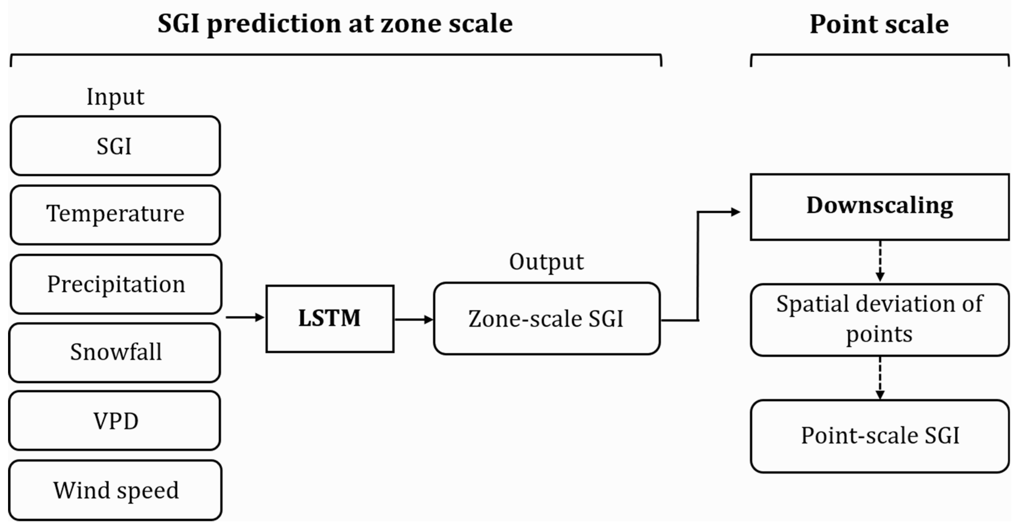
Taken together, this study aimed to develop a multi-scale groundwater-level-based drought prediction model utilizing long short-term memory (LSTM) and various hydrometeorological data (Figure 1). Focusing on the groundwater system of Jeju Island, individual models were constructed for each sub-watershed defined as a zone, totaling 16 zones. Using the LSTM model, the standardized groundwater level index (SGI) was forecasted using the daily temperature, precipitation, snowfall, vapor pressure deficit (VPD), wind speed, and preceding SGI values as input data. Additionally, the zone-scale predicted values were downscaled to point-scale values at each groundwater monitoring well within the zone, achieved by applying the averaged spatial deviation of each point-scale value over the preceding days to the zone-scale predicted value.
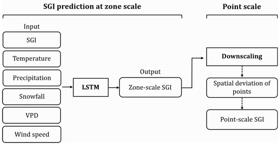
Figure 1.
Schematic diagram of multi-scale SGI prediction model based on LSTM.
The specific objectives of this study were as follows:
- Analyze the impact of meteorological factors on groundwater level fluctuations.
- Evaluate the accuracy of groundwater level prediction using LSTM models.
- Implement downscaling techniques to translate zone-scale prediction values into point-scale prediction values.
2. Materials and Methods
2.1. Hydrometeorological Data
2.1.1. Gridded Meteorological Data
We obtained the daily average temperature, precipitation, snowfall, and VPD data from MK-PRISMv2.1, which is 1 km gridded meteorological data provided by the Korea Meteorological Administration [34]. MK-PRISM is based on a Korean parameter-elevation regression on independent slopes model (PRISM), which adjusts high-resolution grid data to a 1 km grid for South Korea. It considers factors such as elevation, distance, topographic facet, and coastal proxy, all of which significantly impact the local climate conditions. We used the daily average temperature, minimum temperature, and precipitation data spanning from 2001 to 2019.
Snowmelt in the mountainous region of Jeju Island plays a crucial role in groundwater recharge [35]. However, obtaining accurate snowfall data for Jeju Island’s mountainous areas poses a challenge, as most available data are concentrated in coastal regions. To address this, we computed snowfall based on a temperature threshold applied to daily precipitation data. Specifically, we aggregated daily precipitation occurrences when the temperature was below 0 °C to estimate the snowfall amounts.
VPD and wind speed are input variables to account for the impact of evapotranspiration on groundwater level fluctuations. VPD is determined as the difference between saturation vapor pressure and actual vapor pressure, calculated using the following formulas:
where is the saturation vapor pressure (kPa), is the actual vapor pressure (kPa), is the near-surface air temperature (°C), and is the dew point temperature (°C). In this study, daily VPD was calculated assuming that the dew point temperature () is approximately equal to the daily minimum temperature.
Since MK-PRISM does not provide wind speed data, we interpolated daily wind speed data from four automated synoptic observing systems (ASOSs) and thirty-two automatic weather stations (AWSs) on Jeju Island to 1 km grids using the ordinary kriging interpolation method.
2.1.2. Groundwater Level Data
The Jeju Special Self-Governing Province, in response to changes in the water environment due to climate change, increasing sources of pollution, and the salinization of coastal aquifers, has established a groundwater monitoring network to manage water resources effectively. This network continuously monitors the groundwater levels and quality. All groundwater observation wells on Jeju Island fall under the jurisdiction of the province, totaling 174 operational wells at the time of writing. The depths of the groundwater wells vary significantly, ranging from 34 m to 550 m, depending on the altitude. Each well is equipped with an automatic data logger that measures the groundwater level, water temperature, and electrical conductivity (EC) every hour [36]. The province provides access to hourly, daily, and monthly groundwater level observation data through an online data distribution platform [37]. For this study, the daily groundwater level data from 163 observation stations were used, ensuring consistency and a comprehensive time series spanning from 2001 to 2019.
2.1.3. Standardized Groundwater Level Index (SGI)
The standardized groundwater level index (SGI) proposed by Bloomfield and Marchant (2013) serves as an index for standardizing groundwater level time series and characterizing groundwater drought. It allows for the evaluation of groundwater level conditions relative to seasonal averages, providing a normalized basis for managing different observation wells with varying groundwater levels and fluctuation ranges. The SGI is derived by transforming groundwater level data into non-parametric normal scores for each calendar month [38].
Instead of the monthly scale, we calculated the SGI on a daily basis to precisely capture the daily fluctuations in groundwater levels. This approach involved employing a non-parametric method to determine the plotting position of daily groundwater level data for each calendar month. Specifically, we used the Cunnane unbiased quantile estimator [39] (Equation (4)), which is expressed as follows:
where is the probability of exceedance, is the rank of the data in descending order, and is the number of data.
We used a non-parametric method, but it is not mandatory to use this approach. Depending on the characteristics of the data, one can use a method that fits the most suitable probability distribution. However, in this study, the groundwater level data varied significantly between the observation wells and across different months, making it challenging to fit an appropriate distribution. Therefore, we opted for the non-parametric method.
We can obtain the normalized SGI value by mapping the estimated cumulative probability value onto the cumulative distribution function (CDF) of the standard normal distribution based on following Equation (5):
where is the groundwater level, is the CDF from the unbiased quantile estimator Equation (4), and is the inverse CDF of the standard normal distribution.
2.2. Model Development
This study endeavored to construct a multi-scale groundwater drought prediction model by integrating deep learning with hydrometeorological variables, as depicted in Figure 1. Initially, an independent LSTM model was formulated to forecast the SGI for each designated sub-watershed, denoted as the zonal-scale SGI prediction model. Subsequently, the predicted zonal-scale SGI values were further downscaled to point-scale values for individual groundwater wells. This downscaling process preserves the preceding spatial variability of point-scale values within each zone.
2.2.1. Importance Analysis of Input Variables
Selecting input variables is a crucial step in developing an artificial neural network model as not all potential input variables contribute equally to model performance. Analyzing the importance of features helps in identifying appropriate input variables [25]. In this study, we assessed the relative importance of each input variable to understand the impact of hydrometeorological factors on groundwater level prediction. Permutation feature importance was calculated for the following variables: temperature, precipitation, snowfall, VPD, wind speed, and preceding SGI across all 16 zones. The permutation feature importance method evaluates the importance of a feature by measuring the decline in model performance when the permutations of that feature are randomly shuffled [40]. When a specific feature is excluded, a larger mean absolute error (MAE) indicates greater importance of the feature in the model. Permutation feature importance has been shown to exhibit less bias compared to other popular explanation methods used in trees. Additionally, because the random feature importance calculations for all permutations are independent, the relationships among features can be maintained [41]. Several previous studies on water resource prediction have utilized permutation feature importance to determine the significance of hydrological characteristics [42,43,44]. In this study, permutation feature importance was averaged over 10 runs to account for slight variations in the results of each run.
2.2.2. Long Short-Term Memory (LSTM)
LSTM was selected as the deep learning algorithm for predicting groundwater levels in this study. Unlike surface water, groundwater responds slowly to meteorological events on the surface, necessitating the consideration of an appropriate lead time for predicting fluctuations. LSTM is well-suited for time series prediction tasks because it can capture and retain information about preceding conditions of input variables, making it suitable for modeling the delayed effects of meteorological factors on groundwater levels [45,46,47].
LSTM is an enhanced structure of RNN designed to handle time-dependent variables in the form of time series [48]. An RNN is a neural network that receives an input sequence and learns a sequential pattern through an internal loop.
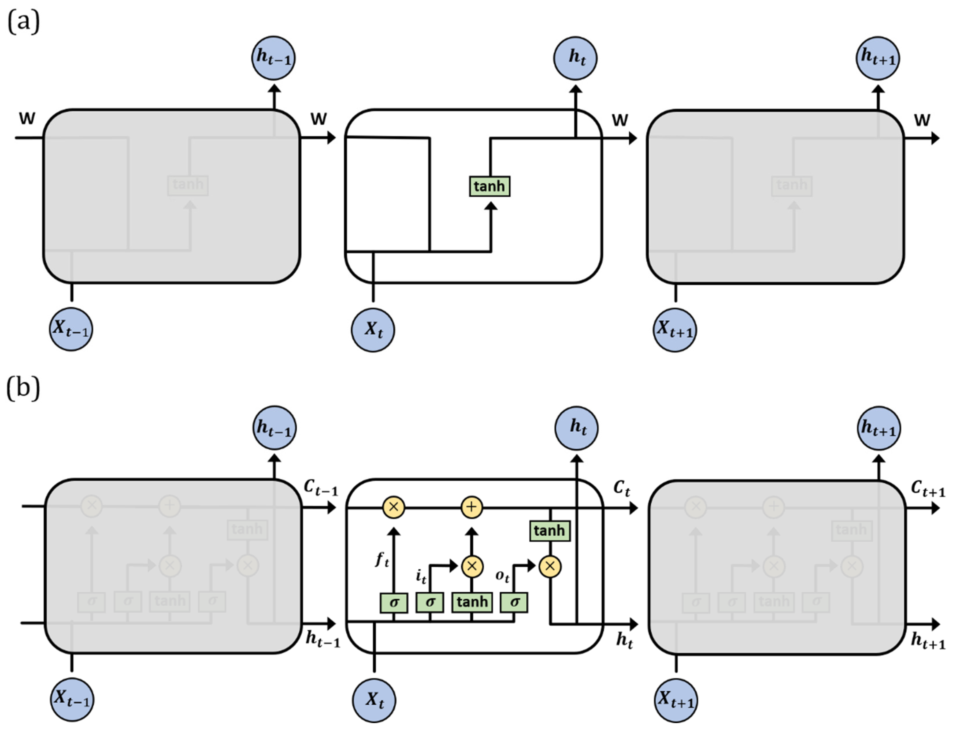
The training of an RNN follows the same sequence as that of a typical neural network, using backpropagation to efficiently compute the gradients of the weight parameters. Backpropagation is a common algorithm for training artificial neural networks that involves the multiplication of the local derivatives of the function in the reverse direction. Based on this backpropagation method, RNNs perform backpropagation through the unfolded network in the time dimension, a process known as back propagation through time (BPTT) [49] (Figure 2a).
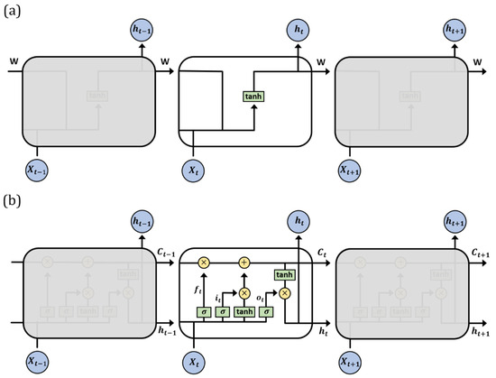
Figure 2.
(a) Chain-like structure of the RNN. (b) Structure of LSTM’s memory block.
However, a challenge arises with vanishing gradients, hindering the model’s ability to capture long-term dependencies. To address this issue, LSTM incorporates a memory block capable of retaining information over extended periods. The memory block comprises a cell state () and three gates: a forget gate (), an input gate (), and an output gate (). These gates manage information flow within the cell state through sequential computations using the following equations (Equations (6)–(11)).
Here, is an input variable at the current time t, is a hidden state, and is a value that determines the amount of new information received in the cell state. The activation function (σ) is the sigmoid function, and tanh is the hyperbolic tangent function. In these equations, U and W are weight matrices, b is a bias vector, and the symbol denotes the element-wise multiplication of two vectors.
Figure 2b shows the flowchart of the LSTM model, and the specific procedure is as follows. First, determines what information to discard from . In the next step, , it is determined which new information to be stored in . The forget gate and input gate control past cell state information and new information. This process updates the past state to create a new . Finally, determine what to output in . The model architecture was implemented using Keras with a TensorFlow backend and scikit-learn in Python 3.9.
2.2.3. Model Calibration
In this study, SGI was predicted using LSTM, with input variables including daily temperature, precipitation, snowfall, vapor pressure deficit (VPD), wind speed, and preceding SGI. In this case, the input included the preceding SGI values, while the output was the SGI value at the target prediction time. Through internal experimentation and trial and error, we determined that the optimal time step for our LSTM model was 4 days.
Data preprocessing involved scaling to transform the data into a suitable format for the model and to enhance its quality. Specifically, the input data were adjusted to fall within the range of −1 to 1. Following preprocessing, 80% of the data spanning from 2001 to 2019 were designated as training data, while the remaining 20% were allocated for testing purposes.
In this study, we employed K-fold cross-validation to assess the model’s performance during training. K-fold cross-validation uses all available data partitions for validation, thereby mitigating potential overfitting issues. However, applying cross-validation to time series data presents unique challenges, as maintaining temporal dependencies is essential. To address this, we adopted a rolling-based cross-validation technique known as time series cross-validation. This approach involves iteratively training the model on subsets of the data and making predictions on subsequent validation data points while preserving temporal order. Specifically, we divided the data into seven subsets and conducted time series cross-validation to evaluate the model performance.
We performed hyperparameter tuning using the grid search method. This approach systematically searches through a specified set of hyperparameter combinations to identify the optimal configuration that minimizes the loss function. By automating the evaluation process across various hyperparameter values, grid search enables efficient optimization of the model compared to manual tuning. In our study, we focused on tuning two key hyperparameters: batch size and the number of epochs. We evaluated the performance of each hyperparameter combination using the Nash–Sutcliffe efficiency coefficient (NSE) as the performance metric. Subsequently, we selected the combination that yielded the highest average NSE across the time series cross-validation folds to optimize the model.
To evaluate the efficiency and predictive ability of all developed models, we used NSE and root mean square error (RMSE). These two statistical criteria are defined as follows:
where is the number of observations, is the observed data, is the average of the observed data, and is the predicted data.
NSE is mainly used to evaluate the prediction accuracy of hydrologic models and ranges from −∞ to 1. An NSE of 1 corresponds to a perfect match between the predicted and observed data, whereas an NSE of less than 0 indicates that the observed mean is a better predictor than the model [50]. RMSE measures the discrepancy between the observed and predicted values. The smaller the RMSE, the lower the error between the observed and predicted values.
2.3. Downscaling for SGI of Points
In our study, we proposed a multi-scale prediction model that included both a zone-scale SGI prediction model using LSTM and a point-scale SGI prediction model. The downscaling method that we propose is similar to the traditional “delta method” [51], which has been commonly used in many studies to downscale climate models. The delta method converts large-scale representative data into small-scale data by using the difference observed between values at two different scales. We implemented a downscaling process to refine the SGI predicted by LSTM at the zone level to the point level within each zone. While zone-level predictions offer broad insights for groundwater management across larger areas, finer-scale predictions at the point level are crucial for the precise management of groundwater resources, especially for individual observation wells. Within a given zone, variations in groundwater levels among different points are influenced by diverse factors such as topographical and geological characteristics. Therefore, downscaling allows us to account for these localized variations and provide more accurate predictions tailored to specific points within each zone.
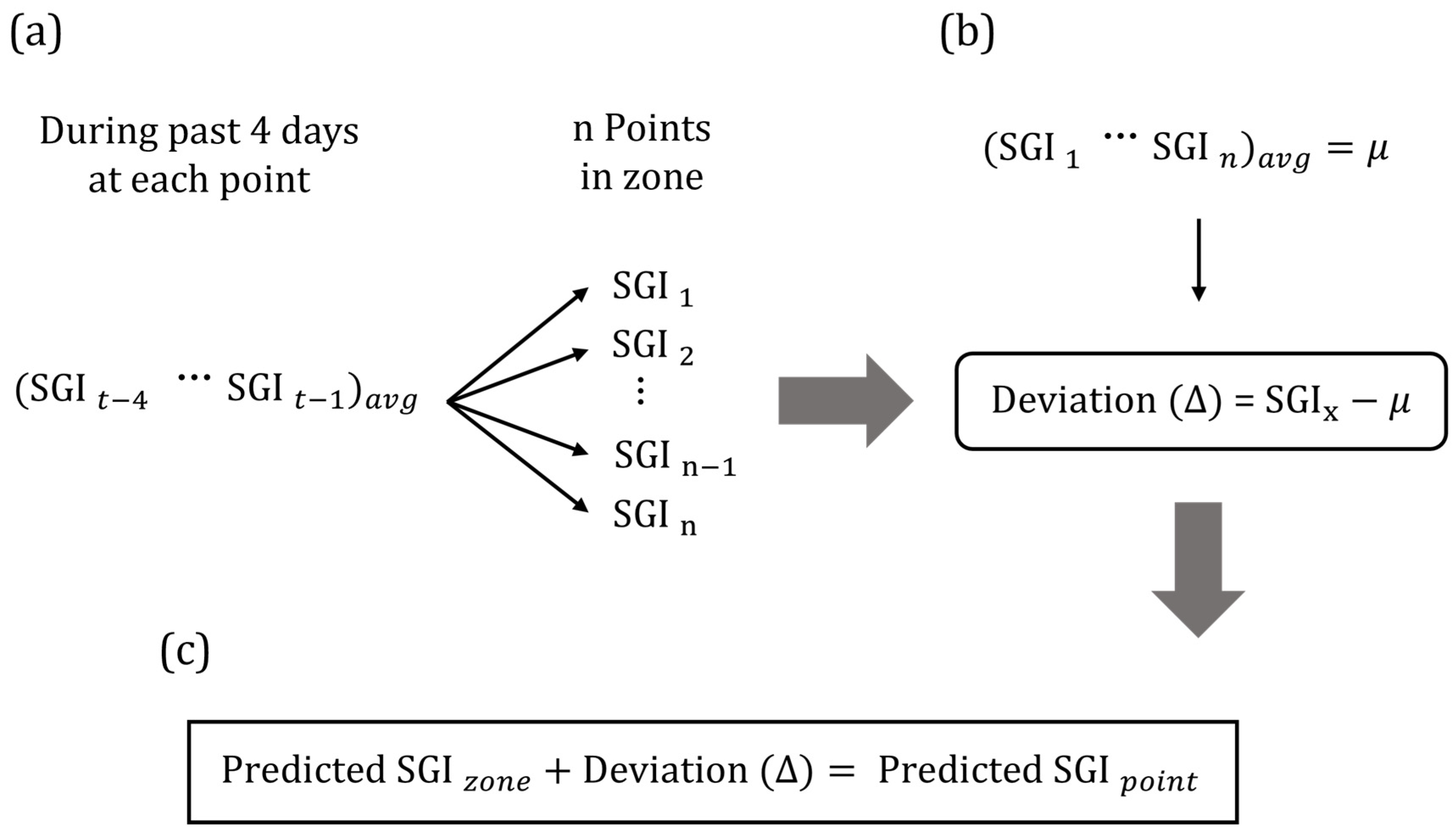
To account for localized variations, we calculated the point-scale SGI by considering the spatial deviation of each point within the zone relative to the zone average SGI value. This involves computing the averaged spatial deviation of each point over the preceding 4 days leading up to the SGI prediction. The downscaling process, described in Figure 3, involves several steps as follows:

Figure 3.
Schematic diagram of the downscaling framework for point-scale SGI at groundwater wells: (a) Calculate the average SGI value for the past 4 days for each point (b) Find spatial deviation for each point (c) Add spatial deviation to calculate zone-scale SGI.
- (a)
- First, calculate the averaged SGI () for each point based on data from the 4-day period preceding the prediction. This step provides a representative SGI value for each specific point.
- (b)
- Calculate the spatial average (μ) of SGI values within the zone, derived from the averages calculated in step (a) across all points within that zone. This spatial average serves as a reference point to understand the overall groundwater condition within the zone.
- (c)
- Determine the spatial deviation (Δ) of each point within the zone by subtracting the spatial average value (μ) from each averaged of each point. This calculation helps quantify how much each point’s groundwater index varies from the zone-wide average.
- (d)
- Finally, to predict the point-scale SGI values, we adjust the zone-scale predicted SGI using deep learning. This adjustment involves adding the spatial deviation (Δ) calculated for each point to the corresponding zone-scale predicted SGI. This method allows for more precise and localized predictions of groundwater levels, leveraging both zone-scale trends and point-specific deviations.
3. Study Area
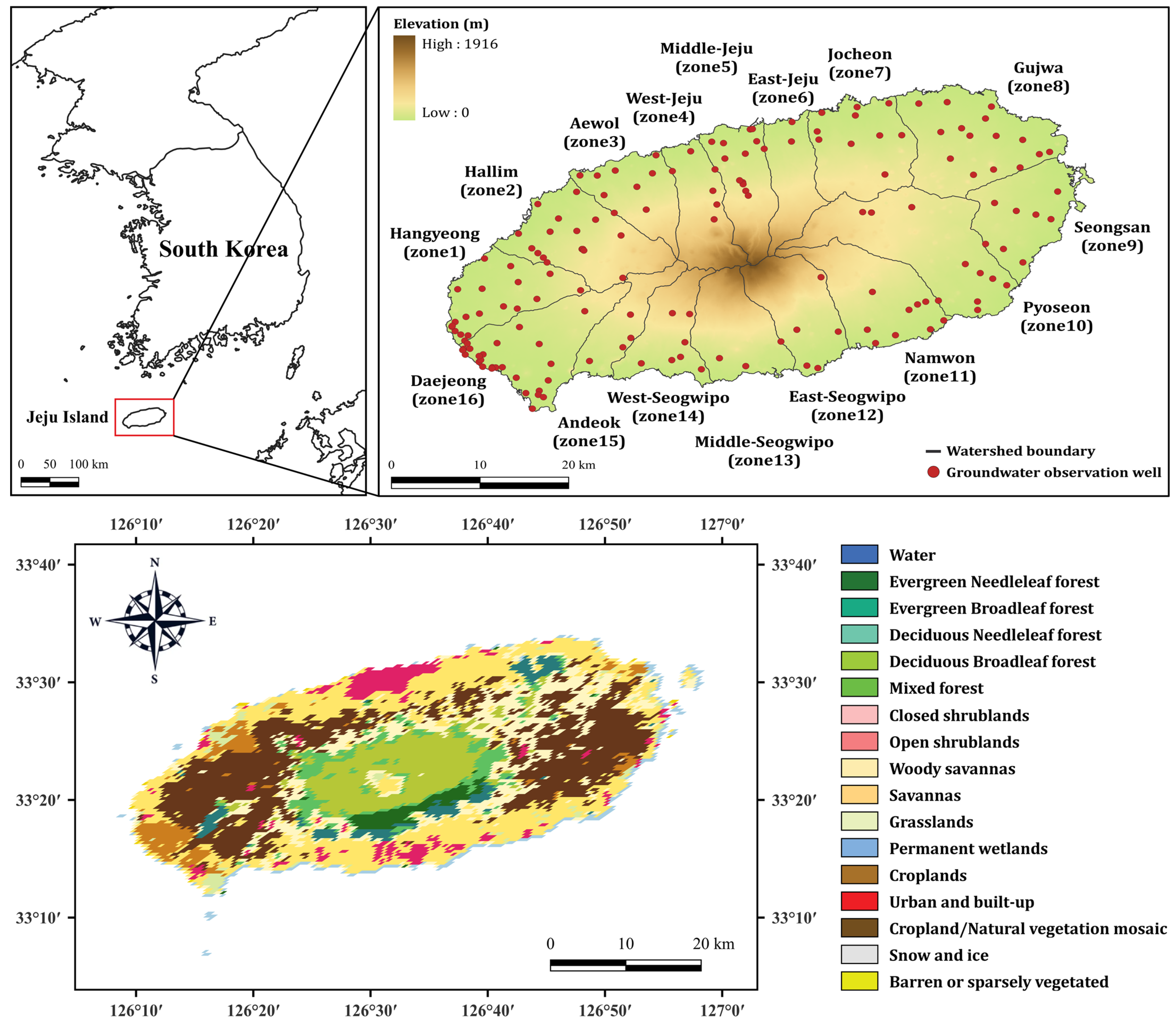
The study area (Figure 4) encompassed Jeju Island (126.1~127.0° E, 33.1~33.6° N), the largest island in South Korea, located approximately 100 km south of the southern tip of the Korean Peninsula. Jeju Island, characterized by its volcanic origin, spans 73 km from east to west and 41 km from north to south, covering a total area of 1825 km2. At the island’s center stands Mt. Halla, a volcanic peak with an elevation of 1950 m, exhibiting a conical shape. The east–west slope of Mt. Halla has a mild gradient of 3 to 5 degrees, contrasting with the steeper north–south slope, which ranges from 5 to 10 degrees.

Figure 4.
Study area overview of Jeju Island including the digital elevation model (DEM) from the Shuttle Radar Topography Mission (SRTM) at a 30 m resolution and land cover data from Moderate Resolution Imaging Spectroradiometer (MODIS) at a 500 m resolution.
Jeju Island, located in the subtropical zone, experiences a warm and humid oceanic climate due to its geographic location and the influence of turbulent currents. Compared to the inland regions of the Korean Peninsula, Jeju exhibits small annual and diurnal temperature variations, high temperatures, and greater precipitation. The central presence of Mt. Halla significantly contributes to the diverse weather conditions across the island. Jeju’s topographical structure extends outward from the central peak of Mt. Halla, and the mountainous influence leads to contrasting weather patterns on windward and leeward sides, resulting in notable differences in temperature and precipitation based on prevailing wind systems. Specifically, the southern and northern slopes, characterized by steep gradients, undergo distinct weather changes.
Jeju Island was formed by volcanic activity in the Cenozoic Era and consists mainly of basalt lava flows with small amounts of pyroclastic and sedimentary rocks [52]. The bedrock, composed of granite or pyroclastic rocks, lies at depths of 155~312 m below sea level. Overlying this bedrock are unconsolidated formations (U-formations), which consist of unconsolidated sedimentary layers. The Seogwipo Formation, which contains shellfish fossils, is widely distributed in the upper part of the U-formations [36]. This sedimentary layer has low permeability and functions as a confined unit [53]. As a result, the abundance and output characteristics of groundwater are influenced by the spatial distribution of the Seogwipo Formation. In the eastern region of Jeju Island, where the Seogwipo Formation is not extensively developed, there is higher permeability compared to other areas. The presence of clinker, a pyroclastic layer situated between lava flows, serves as a significant aquifer [54]. The island’s hydrogeological structure is characterized by high permeability and porosity, contributing to substantial rates of groundwater recharge. Jeju’s groundwater recharge is estimated at 1653 × 106 m3/year, which accounts for 45.8% of the total precipitation [52]. Due to its storage capacity, Jeju experiences minimal decline in groundwater levels relative to pumping rates, resulting in a relatively high specific capacity [53].
The groundwater basin of Jeju Island is divided into 16 watersheds (Hangyeong, Hallim, Aewol, West-Jeju, Middle-Jeju, East-Jeju, Jocheon, Gujwa, Seongsan, Pyoseon, Namwon, East-Seogwipo, Middle-Seogwipo, West-Seogwipo, Andeok, Daejeong). For the efficiency of analysis, the Jeju Special Self-Governing Province established groundwater basins according to hydrogeology and topographical conditions. For the sake of clarity in this study, zones were numbered sequentially from 1 to 16 in a clockwise manner starting from the Hangyeong Basin to the Daejeong Basin.
4. Results and Discussion
4.1. Climate Analysis of Jeju Island
We analyzed the climate of Jeju Island from 2001 to 2019 using gridded meteorological data. The average annual temperature of Jeju is 14.1 °C, which is 1.4 °C higher than the national average of 12.7 °C. The annual precipitation is 2272.2 mm, significantly surpassing the national average of 1306.3 mm by 965.9 mm.
Figure 5 shows the average and standard deviation of the monthly temperature and precipitation on Jeju Island from 2001 to 2019. The seasonal temperature ranges from a high of 25.1 °C in August, the warmest month, to a low of 3.3 °C in January, the coldest month. Summer precipitation (June, July, and August) comprises approximately 40% of the annual total, while winter precipitation (December, January, and February) is comparatively lower, constituting about 11% of the annual rainfall.
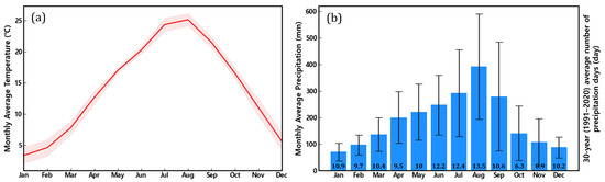
Figure 5.
Climate analysis using gridded meteorological data from 2001 to 2019: (a) monthly average temperature and (b) monthly average precipitation with average number of precipitation days presented as numbers in the lower part of bars.
As a result of analysis using gridded meteorological data, Jeju Island displays distinct climatic variations between its eastern and western slopes, centered around Mt. Halla. When segmented by zone, the average annual temperature in Hangyeong and Daejeong were notably higher at 15.7 °C and 15.6 °C, respectively. Conversely, East-Seogwipo, West-Jeju, and Middle-Jeju experienced relatively cooler temperatures at 12.2 °C, 12.4 °C, and 13.2 °C, respectively. Annual precipitation exhibited considerable disparities across the island’s zones. East-Seogwipo received the highest annual rainfall at 3236.3 mm, followed by Namwon at 2842.9 mm, and Pyoseon at 2750.8 mm, all exceeding 2700 mm annually. In contrast, Hangyeong and Daejeong experienced lower precipitation levels at 1411.3 mm and 1553.1 mm, respectively. Particularly noteworthy is the fact that East-Seogwipo, with the highest precipitation, received more than double the rainfall of Hangyeong, which experienced the least precipitation. These findings underscore the significant spatial variability in temperature and precipitation across Jeju Island, influenced by its unique geographic features and topography.
4.2. Zone-Scale SGI Prediction
4.2.1. Importance of Input Variables for Each Zone
We assessed the importance of input variables including SGI, temperature, precipitation, snowfall, VPD, and wind speed using permutation feature importance. Figure 6 illustrates a heatmap that ranks the significance of these factors across all zones, highlighting the consistent prominence of preceding SGI across the island. Unlike surface water, groundwater exhibits a longer travel time to reach and outflow from the aquifer, resulting in comparatively minor temporal variability. Consequently, the previous SGI values exhibited a high degree of similarity with the present groundwater levels across all zones. Following SGI, precipitation emerged as the next most important factor influencing groundwater levels in most zones, with the exception of zones 13, 14, and 15. Precipitation plays a crucial role in groundwater recharge, particularly in the eastern region where the Seogwipo Formation, characterized by low permeability, is less developed. On the other hand, zones 13, 14, and 15 in the western region showed diminished precipitation effects. This area, known for agriculture, experiences predominant fluctuations in groundwater levels driven by groundwater extraction rather than precipitation [55]. Temperature emerged as the second most important after precipitation, with its significance gradually diminishing in relation to wind speed, VPD, and snowfall. Following the feature importance analysis, minimal distinctions were observed in the contributions of the remaining meteorological factors, aside from SGI. Therefore, it is noteworthy that all six hydrometeorological factors considered for characteristic importance are valuable as input variables for the deep learning-based SGI prediction model.
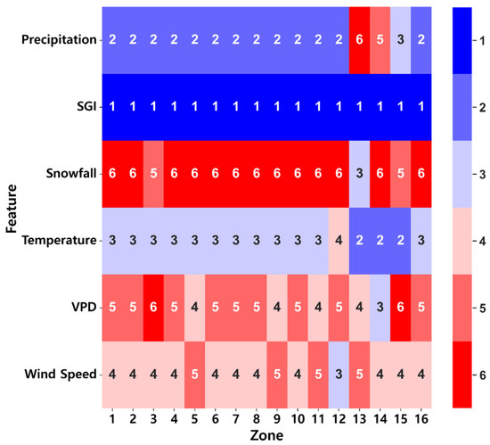
Figure 6.
Ranking of the importance of input variables for each sub-watershed zone, with “1” indicating the most important variable.
4.2.2. SGI Prediction Results
We constructed individual LSTM-based SGI prediction models for each zone and trained them using daily input data including temperature, precipitation, snowfall, VPD, wind speed, and SGI. While in the training phase, each model went through a cross-validation process to optimize the hyperparameters. We conducted a comprehensive evaluation of model performance based on a grid search approach, exploring various combinations of hyperparameters (batch size and epoch) to determine optimized settings for each model. The optimal hyperparameters for each model in groundwater level prediction are presented in Figure 7. Among the batch sizes {64, 128, 256, 512}, 64 and 128 emerged as the optimal hyperparameters for most models. Regarding epoch values, several hyperparameters among {100, 130, 150, 170, 200, 230, 250, 270, 300} were identified as optimal, with 150, 230, and 250 being the predominant choices across the models.
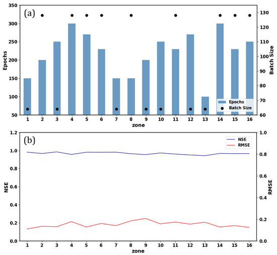
Figure 7.
Optimal hyperparameters and performance statistics for each zone-scale model: (a) epochs and batch size, (b) NSE and RMSE.
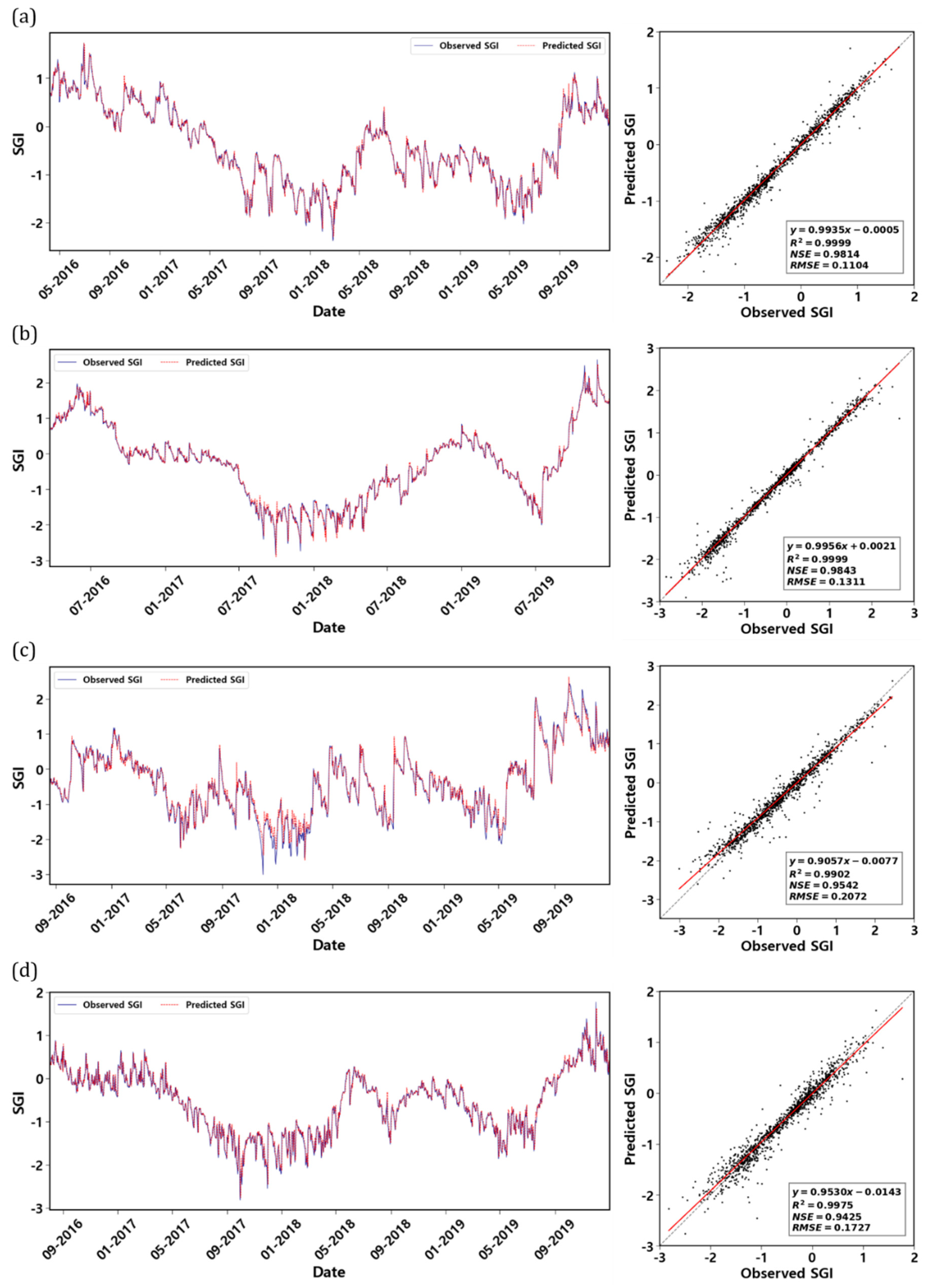
To assess the performance of the optimized model, we simulated the daily SGI prediction for each zone during the test period. We used NSE and RMSE as performance evaluation metrics. Figure 7 shows the results of the model performance evaluation using test data, along with the optimal hyperparameters for each model. Notably, NSE values of 0.9 or higher were observed across all zones. The average value of NSE was 0.9671, indicating very high accuracy. When examined by zone, the highest NSE was 0.9843 in zone 3, while the lowest was 0.9425 in zone 13. Additionally, RMSE exhibited consistently low values, with the lowest in zone 1 at 0.1104, and the highest in zone 9 at 0.2072. The average RMSE across all zones was 0.1519, highlighting the excellent performance of the LSTM-based SGI prediction model. The excellent performance of LSTM in predicting the groundwater level time series shown in the results of this study is similar to the results of several studies predicting groundwater level using LSTM [45,47,56].
Figure 8 displays a time series graph and scatter plot comparing the observed SGI with the predicted SGI throughout the test period for zone 1, zone 3, zone 9, and zone 13. The selection included the results of the two most accurate zones (zone 1 and zone 3) and the two least accurate zones (zone 9 and zone 13). All of the results from other zones are presented in Figure S1 in the Supplementary Materials. The time series revealed that the overall fluctuations in both the observed and predicted SGI values across all zones shared similar trends. It further demonstrates the model’s capability to effectively capture minute fluctuations in groundwater levels across most zones. Remarkably, even in zones with relatively low accuracy, the model exhibited excellent predictive performance on highly variable groundwater fluctuations.
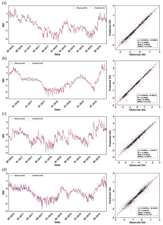
Figure 8.
Time series graphs and 1-on-1 scatter plots comparing the observed and predicted SGI of zones in the test period: (a) zone 1, (b) zone 3, (c) zone 9, and (d) zone 13.
The high prediction accuracy of the model is more clearly illustrated in the one-on-one scatter plot. The relationship between the observed and simulated SGI was elucidated through linear regression analysis, enhancing clarity. Calculating the coefficient of determination (R2) from the linear regression equation yielded values close to 1 in all zones, indicating that the predicted SGI fit the observed values with a high degree of accuracy.
In previous studies that predicted the groundwater levels on Jeju Island, the focus was solely on predicting the groundwater levels of individual observation wells [46,57]. In contrast, this study accurately predicted zone-scale SGI using data from almost all groundwater observation wells on Jeju Island, enabling the establishment of a comprehensive and efficient groundwater management system.
The SGI prediction models for several zones including zones 11 to 16 showed somewhat lower accuracy compared to other zones. Notably, the diminished accuracy of the zone 13 model is likely due to insufficient data. Zone 13 only has three observation wells, fewer than other zones, and the available groundwater level data are shorter. This limited dataset may lead to overfitting during model training, consequently restricting the model’s performance during the test period. Thus, additional data from observation wells are essential to derive more accurate results and better represent groundwater level fluctuations. Nevertheless, our results demonstrate significant potential in predicting groundwater-level-based drought.
The southern regions, encompassing zones 11 to 16, have a higher concentration of groundwater wells than other regions, primarily due to extensive agricultural activities. In particular, zones 11 and 16 alone contribute to approximately 40% of the total number of wells on Jeju Island. Here, the ratio of agricultural water use to the total groundwater volume stands at 40.1%, ranking as the second-largest category after domestic water use. In addition, zones 11 to 14 exhibited a significant prevalence of polytunnel farming, constituting 4.0~8.3% of the watershed area [19]. Polytunnel farming increases the impervious area, leading to an increased direct runoff ratio. These anthropogenic factors, particularly in the southern region, significantly contribute to fluctuations in the groundwater levels, and consequently increase the uncertainty in the model. Therefore, future studies aiming to estimate the groundwater level fluctuation in this region may benefit from focusing on anthropogenic factors such as population density, groundwater withdrawal amount, and impermeability, in addition to meteorological variables.
4.2.3. Predicted SGI Map by Zone
Figure 9 shows the results of the monthly average SGI predictions for four representative months during the test period. The selection included two dry and two wet months, demonstrating relatively significant spatial variability compared to other months. The SGI values exhibited noticeable differences between zones, with substantial variability even among neighboring zones.
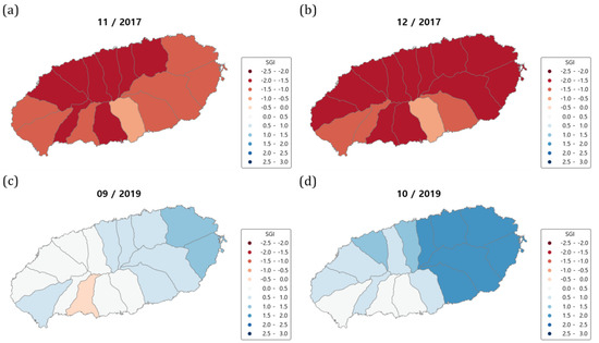
Figure 9.
Monthly SGI predicted map for each zone: (a) November 2017, (b) December 2017, (c) September 2019, and (d) October 2019.
In the results for November and December 2017 (Figure 9a,b), Jeju Island exhibited remarkably low SGI values, corresponding to the severe drought experienced on the island that year. The total precipitation in 2017 amounted to 1053.7 mm, which was only 61.6% of the normal value of 1710.3 mm. Notably, the annual precipitation in the northern region reached 773.3 mm, approximately half of the normal value of 1497.6 mm. This marked the lowest precipitation amount since weather observations began in 1923. Although precipitation was generally low throughout 2017, the summer season was particularly deficient, receiving only 49% of the normal value. Additionally, November recorded minimal precipitation, falling below 20% of the normal amount, primarily due to the prevalence of high-pressure systems. Historically, groundwater levels on Jeju Island are typically at their lowest during spring (April to May) and show an increase during summer (June to July). However, the persistence of drought conditions, stemming from inadequate summer precipitation, extended until the conclusion of 2017. Given that summer precipitation significantly contributes to the annual total, a deficit during this critical period prolongs drought impacts into subsequent years, irrespective of autumn precipitation patterns. The average annual temperature in 2017 was 0.7 °C higher than the normal mean of 16.2 °C. Notably, the temperatures in July and August were 1.5 °C higher than normal. These elevated temperatures led to heatwaves and tropical nights, which likely heightened the groundwater demand, exacerbating drought conditions across the region.
On the other hand, the graphs for September and October 2019 (Figure 9c,d) show elevated values of SGI of 0 or higher in most zones. In 2019, Jeju Island recorded an average annual temperature of 17.1 °C, marking the second-highest since 1961. With the exception of June to September, which were characterized by frequent rainfall during the rainy season and typhoons, temperatures for most months surpassed the normal range by 0.8 to 1.8 °C. Despite the relatively high average annual temperature, stable groundwater levels were observed in autumn, likely due to frequent summer precipitation and the influence of numerous typhoons. The average annual accumulated precipitation for 2019 was 2095.1 mm, surpassing the normal value. Although precipitation from January to April and November was below normal, July, September, October, and December experienced above-normal precipitation. Notably, both July and September recorded historically high levels of precipitation, ranking among the top fifth and third in history, respectively.
The groundwater level shows a close relationship with preceding hydrometeorological factors [12]. Meteorological conditions in one month can influence groundwater level fluctuations in subsequent months, as clearly illustrated in the results of this study. For instance, Figure 9 demonstrated lower SGI values in December compared to November 2017, a period characterized by minimal precipitation. In contrast, the SGI for the following month, October, exhibited higher values than September 2019, a period marked by substantial precipitation.
Climate change has disrupted the regularity of the drought cycle, leading to more frequent occurrences of localized droughts [58]. Currently, the operational drought information system provides monthly SGI values based on administrative districts, without subdivision into watershed levels. This limitation impedes accurate identification of the increasingly common localized droughts. Therefore, there is a pressing need to understand groundwater level fluctuations at the sub-watershed level rather than relying solely on administrative districts. The proposed model not only enhances the efficiency of groundwater management by predicting groundwater levels at the watershed level, but also facilitates the management of regionally specialized groundwater resources.
4.3. Point-Scale Prediction with Downscaling
4.3.1. Evaluation of Point-Scale SGI Prediction
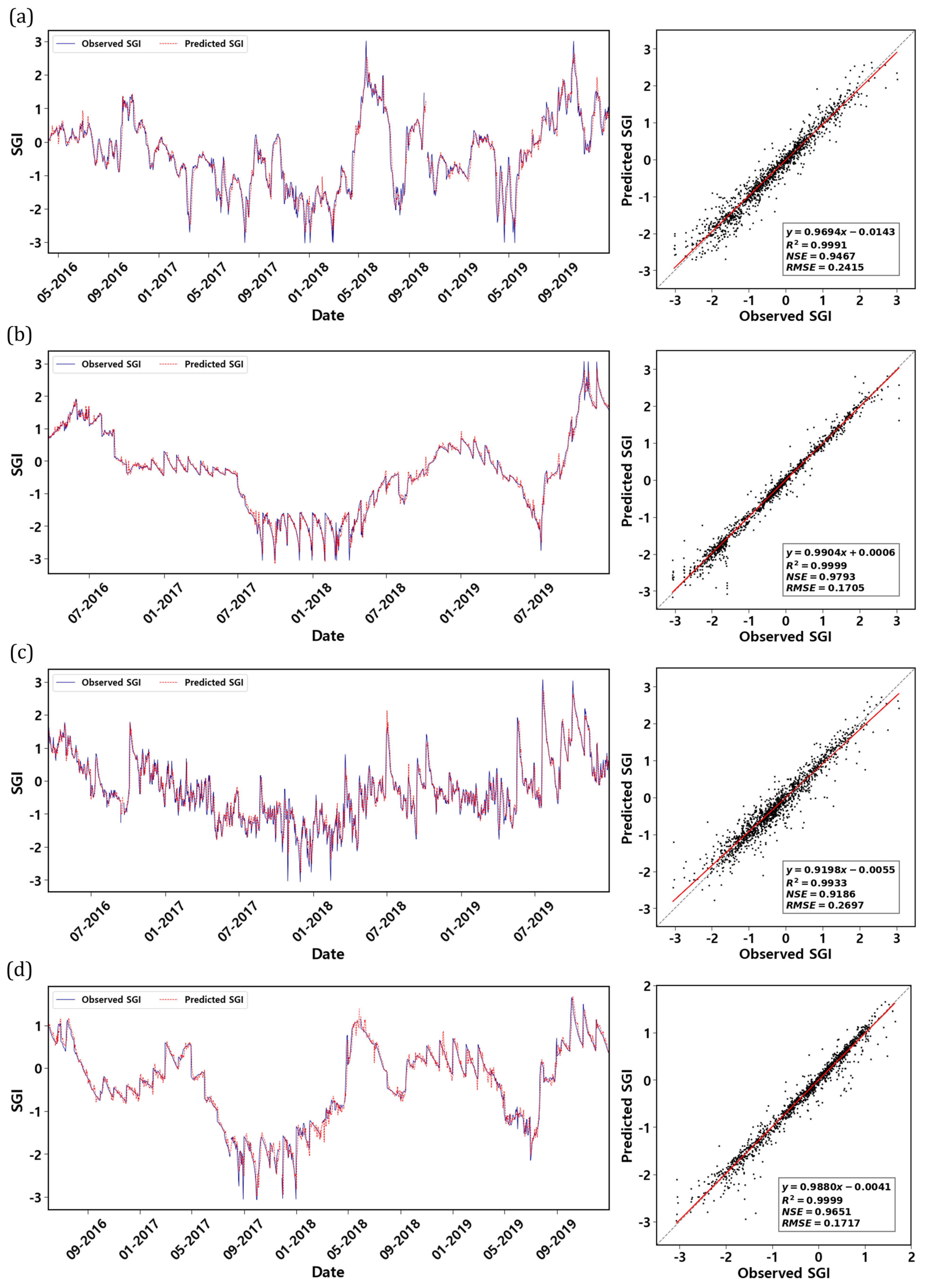
We proposed a multi-scale SGI prediction model that involves downscaling zone-scale SGI, predicted using LSTM, to point-scale SGI. Figure 10 illustrates the observed SGI along with the predicted SGI derived from downscaling over a test period at four observation wells. Both the time series graph and scatterplot showed that point-scale SGI prediction using downscaling performed reasonably well. Point-scale SGI prediction results (Figure 10) showed robust prediction of SGI trends across most observation wells, effectively capturing detailed fluctuations in the groundwater level. Evaluation metrics underscore the high accuracy of the point-scale SGI well. NSE for the representative observation wells consistently exceeded 0.9, while the RMSE remained below 0.3. In addition, R2 calculated through regression analysis surpassed 0.99 in all cases, affirming the model’s high accuracy.
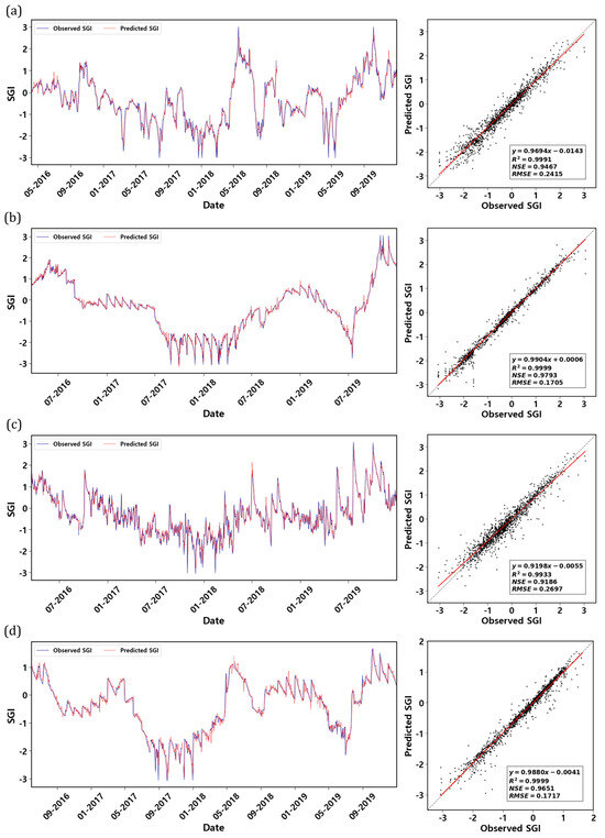
Figure 10.
Time series graphs and 1-on-1 scatter plots comparing the predicted and observed SGI of the groundwater well during the test period: (a) JD Yongsu 1 (zone 1), (b) JM Shineum (zone 3), (c) JD Handong 2 (zone 8), and (d) JW Jungmun 1 (zone 14).
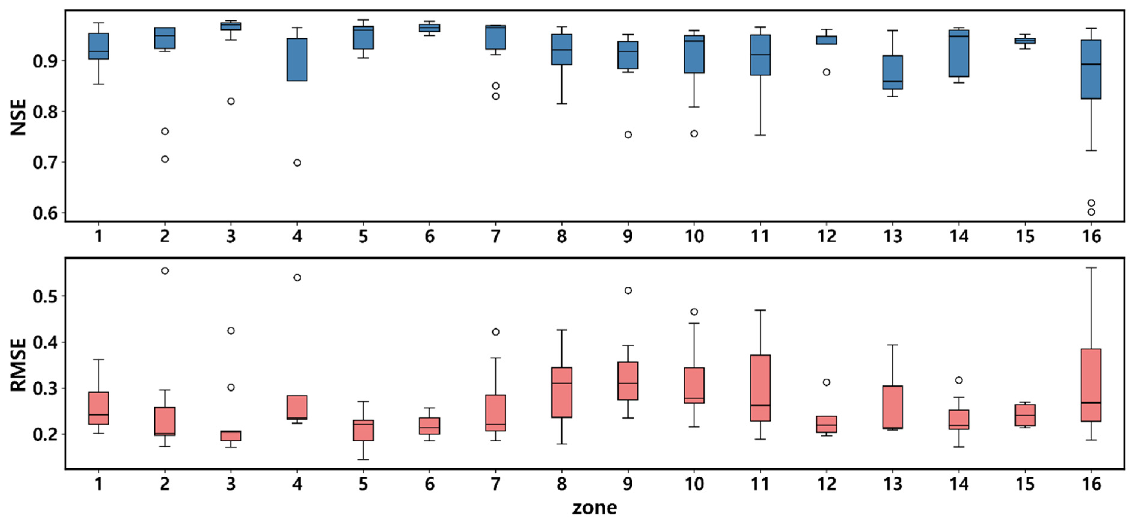
Figure 11 presents the box plots depicting the NSE and RMSE of point-scale SGI for each zone. Across most observation wells in the zones, the NSE of SGI exceeded 0.7, accompanied by consistently low RMSE values, although a few observation wells exhibited slightly lower accuracy. Overall, the box plot results indicate reasonably high accuracy in point-scale SGI prediction. Notably, zone 11 and 16 showed a relatively low accuracy. As mentioned earlier, these areas are characterized by extensive groundwater well development, with significant abstraction for agricultural purposes likely contributing to the observed deviations.
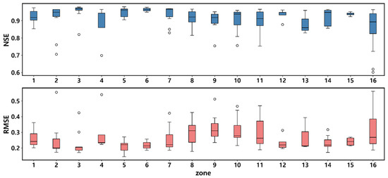
Figure 11.
Box plots showing the NSE and RMSE of the point-scale SGI for all 16 zones. Whiskers extend to 1.5 times the interquartile range (IQR) from the first and third quartiles (Q1 and Q3), with outliers shown individually.
We predicted the point-scale SGI by incorporating spatial deviation, which captures variations over the preceding 4 days, across all observation wells. However, our approach may result in marginal errors when the spatial variability of SGI changes compared to the average of the past 4 days. This situation can occur when the region experiences different spatial patterns of precipitation. Additionally, the recharge rate of groundwater between observation wells varies according to the geological characteristics as well as topographical features such as elevation and slope. As a result, the lag time of groundwater levels may differ for each observation well, resulting in spatial variability in groundwater-based drought assessments.
Nonetheless, our study’s results are similar to those of other studies that have used deep-learning models for individual groundwater wells [46,57,59]. The high predictive performance of point-scale SGI prediction demonstrates the efficacy of our proposed SGI downscaling framework. By employing the multi-scale SGI prediction model, we can efficiently forecast SGI at multiple points without the need for extensive individual well modeling. This approach facilitates the precise and expedient prediction of groundwater-based drought across a more granular spatial range within the watershed unit.
4.3.2. Spatial Analysis of Point-Scale SGI Prediction
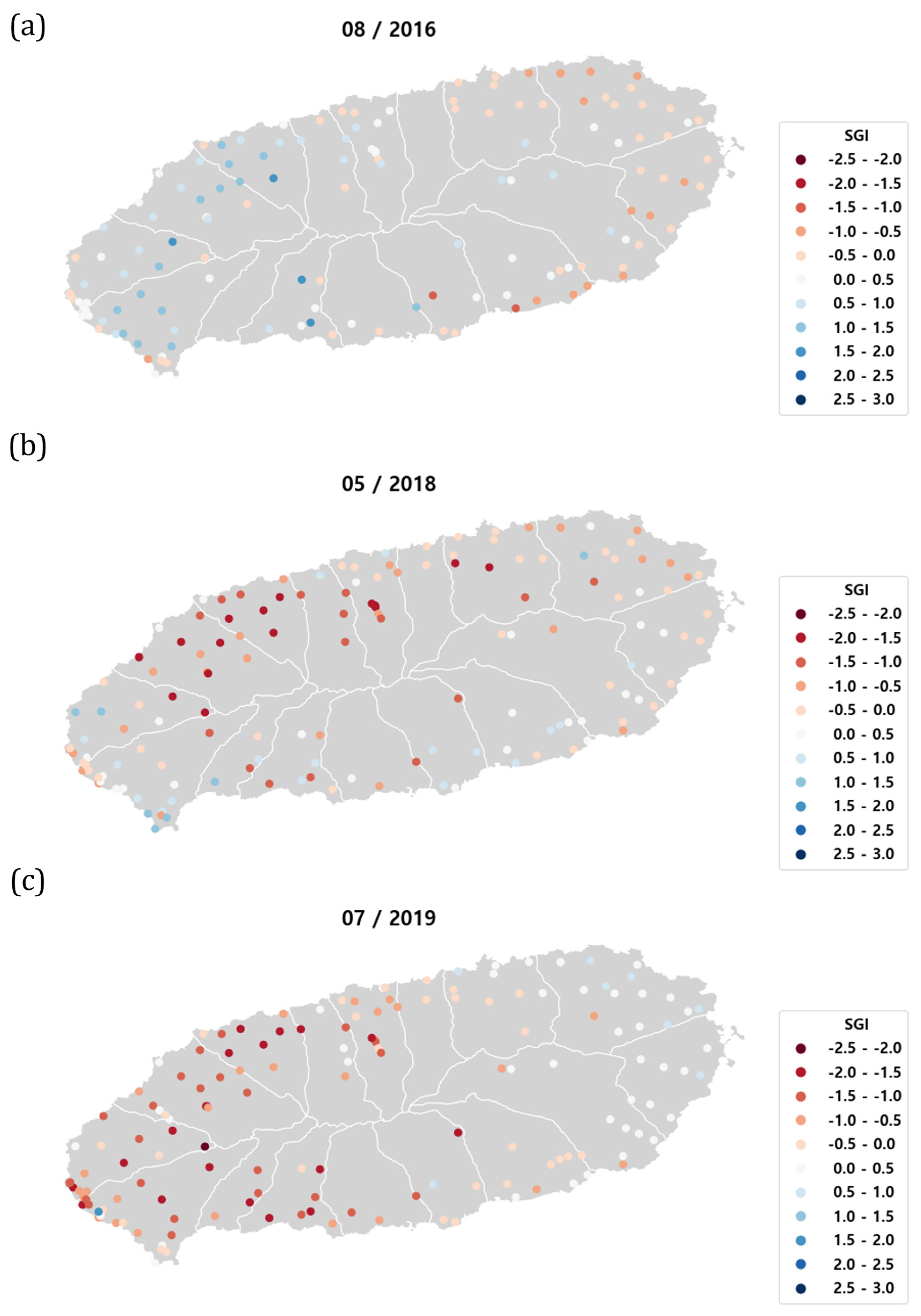
We calculated the monthly average value of daily point-scale SGI values across all observation wells. Figure 12 represents the monthly average point-scale SGI map for the three selected months, showing relatively significant variability across the region. The graph depicts variations in SGI across zones and individual points, which can be attributed in part to differences in precipitation patterns resulting from the topographical effect of Mt. Halla.
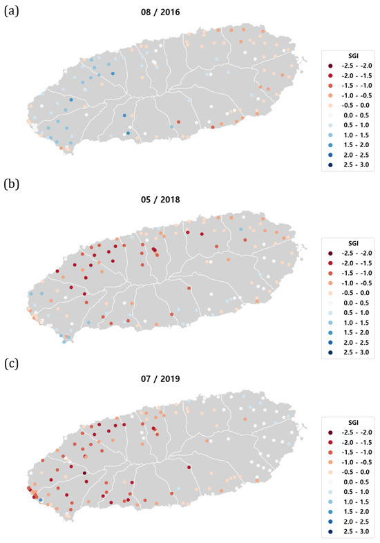
Figure 12.
Monthly SGI predicted map by point: (a) August 2016, (b) May 2018, and (c) July 2019.
In the August 2016 graph (Figure 12a), the western region showed high SGI values while the eastern region showed low SGI values. During this period, precipitation across Jeju Island was below normal due to continuous influence from the North Pacific high pressure and the Chinese mainland high-pressure systems. However, there was a notable disparity in precipitation between the western and eastern regions. The western region including zones 1 to 5 and 13 to 16 experienced precipitation ranging from 76.4 to 172 mm, which amounted to 23 to 61% of the normal levels. In contrast, the eastern region, comprising zones 7 to 12, recorded relatively low precipitation levels of 81.4 to 108.5 mm, accounting for only 17 to 32% of the normal levels. This precipitation discrepancy contributed to the contrasting SGI values across the region.
In the May 2018 graph (Figure 12b), the SGI values were notably lower in the northwestern and eastern regions, while the southern and western regions exhibited relatively high values. The average temperature in May 2018 exceeded normal levels, particularly in the northern and western regions, where temperatures were 1 °C higher than usual. Additionally, May 2018 experienced above-average precipitation, with an increased frequency of rainy days. The influence of the southwest air current, coupled with the topographical effects of Mt. Halla, led to substantial precipitation in the southern and western regions, recording 356.1 mm and 256.7 mm, respectively, along with a higher number of rainy days compared to typical patterns. However, the northern area received less precipitation compared to other regions, notably affecting Jocheon Basin (zone 7), which experienced a precipitation level of only 53% of normal. Additionally, the northern region including the Aewol Basin (Zone 3) is experiencing the most rapid urbanization due to dense tourist facilities and high population density. Urbanization is accompanied by a reduction in natural green spaces and an increase in impervious surfaces. These changes in the land surface ultimately alter the groundwater flow system, leading to increased surface runoff and decreased groundwater recharge. Urban surfaces covered with materials such as concrete and asphalt store a significant amount of heat due to their high thermal inertia [60,61]. Moreover, the lack of vegetation results in rapid surface water runoff, reducing evapotranspiration in urban areas, and consequently decreasing the availability of moisture from locally generated precipitation [62]. Industrial development and population growth increase the demand for commercial and domestic water. The high domestic water demand in the northern region boosts groundwater pumping, impacting the groundwater levels [63]. Therefore, the increase in surface runoff, reduction in precipitation, and heightened groundwater demand due to urbanization likely contribute to the observed low SGI values in the northern region.
In the July 2019 graph (Figure 12c), the SGI values exhibited a distinct contrast between the eastern and western regions of Jeju Island. During this period, the precipitation levels across the island varied significantly between these two regions. Precipitation in the eastern region reached 516.5 mm, nearly double the normal value of 283.2 mm. In contrast, the western region received relatively scant precipitation, recording only 191.3 mm. This marked a significant difference in precipitation levels, with the eastern region receiving approximately 2.7 times more precipitation than the western region.
Referring to Figure 12, the distribution of SGI values from observation wells showed a pattern resembling concentric circles as they approach the coastline of Jeju Island. This phenomenon is opposite to what was observed around Mt. Halla, and can be attributed to Jeju Island’s significant regional variations and topographical effects. The altitude of Jeju Island gradually decreases from the center toward the coast. Consequently, the average annual precipitation in the southern region is about twice that of the western region, and the mountainous areas in the central region receive more than twice the amount of precipitation compared to the coastal areas. The increase in precipitation per unit of elevation is greater in the southern and eastern regions compared to the northern and western regions [52,64]. Additionally, low-altitude coastal areas with high population densities experience significant groundwater extraction due to human activities. Conversely, mountainous regions with steep hydraulic slopes benefit from substantial precipitation recharge, resulting in limited abstraction effects.
5. Summary and Conclusions
This study developed a multi-scale groundwater-based drought prediction model operating at both zone and point scales. Specifically, we constructed a deep learning-based model to forecast SGI values for each sub-watershed (zone), utilizing key hydrometeorological variables such as temperature, precipitation, snowfall, vapor pressure deficit (VPD), wind speed, and preceding SGI values as input factors. Additionally, we applied spatial deviation to downscale the predicted zone-scale values to individual groundwater well values within each zone.
We utilized permutation feature importance to calculate the relative contribution of hydrometeorological variables, thereby assessing their impact on groundwater level fluctuations. Our findings revealed a descending order of importance, with preceding SGI and precipitation exerting the greatest influence, followed by temperature, wind speed, VPD, and snowfall. These findings highlight the critical role of preceding groundwater conditions and precipitation patterns in shaping groundwater level dynamics on Jeju Island.
Both the zone-scale and point-scale SGI prediction models demonstrated remarkable accuracy in forecasting groundwater levels on Jeju Island. The zone-scale model, utilizing LSTM, adeptly captured rapid fluctuations and overall trends in groundwater levels. It achieved high-performance metrics with an average NSE of 0.9671 and RMSE of 0.1519, indicating excellent predictive capabilities. Similarly, the point-scale model, which involved downscaling predictions from the zone-scale model to individual observation wells, demonstrated precise forecasting of the groundwater level fluctuations. This model captured even subtle variations across most observation wells with commendable precision, ensuring reliable predictions at a localized level.
Analysis of the spatial distribution characteristics revealed distinct variations in SGI across different zones, and in many instances, within the same zone among observation wells. These differences are largely attributed to the topographical influence of Mt. Halla. The distribution of SGI is primarily shaped by precipitation patterns, with additional variations potentially influenced by human activities such as agricultural practices.
While our proposed model successfully predicted groundwater level fluctuations using hydrometeorological factors, it is increasingly recognized that climate change and human activities such as urbanization and industrial development significantly influence these fluctuations. Therefore, integrating anthropogenic factors such as population density, groundwater withdrawal rates, and land impermeability into the model alongside meteorological variables is expected to yield more accurate results.
The multi-scale prediction model introduced in this study offers a dual capability to generate zone-scale and point-scale groundwater-based drought predictions efficiently. By providing detailed spatial information on groundwater drought, our model enables accurate prediction and preparedness for the increasingly frequent localized droughts anticipated in the future. Particularly, the predictions derived from our multi-scale model hold significant value across various sectors including agriculture, drinking water provision, tourism, and industries reliant on groundwater resources. Moreover, it provides a foundation for stakeholders and policymakers to formulate sustainable groundwater management strategies for the future, especially in regions where groundwater plays a pivotal role.
Supplementary Materials
The following supporting information can be downloaded at: https://www.mdpi.com/article/10.3390/w16142036/s1, Figure S1: Time series graphs and 1-on-1 scatter plots comparing the observed and predicted SGI of zones in the test period: (a) zone 2, (b) zone 4, (c) zone 5, (d) zone 6, (e) zone 7, (f) zone 8, (g) zone 10, (h) zone 11, (i) zone 12, (j) zone 14, (k) zone 15, and (l) zone 16.
Author Contributions
Conceptualization, D.K. and K.B.; Methodology, D.K. and K.B.; Validation, D.K. and K.B.; Formal analysis, D.K. and K.B.; Investigation, D.K. and K.B.; Resources, K.B.; Data curation, D.K. and K.B.; Writing—original draft, D.K. and K.B.; Writing—review & editing, D.K. and K.B.; Visualization, D.K. and K.B.; Supervision, K.B.; Project administration, K.B.; Funding acquisition, K.B. All authors have read and agreed to the published version of the manuscript.
Funding
This work was supported by a National Research Foundation of Korea (NRF) grant funded by the Korean Government (MSIT) (No. NRF-2022R1F1A1074164 and NRF-2022R1A4A3032838).
Data Availability Statement
The gridded meteorological data used in this study can be obtained through the online data distribution system of the Korea Meteorological Administration: http://www.climate.go.kr/home/CCS/contents_2021/32_2_user_analysis_past.php (accessed on 15 January 2024). The groundwater level data from monitoring wells on Jeju Island can be retrieved through the Jeju Groundwater Data Distribution Platform: https://water.jeju.go.kr (accessed on 1 March 2024).
Conflicts of Interest
The authors declare that they have no known competing financial interests or personal relationships that could have appeared to influence the work reported in this paper.
References
- Alley, W.M.; Healy, R.W.; LaBaugh, J.W.; Reilly, T.E. Flow and storage in groundwater systems. Science 2002, 296, 1985–1990. [Google Scholar] [CrossRef] [PubMed]
- Döll, P.; Hoffmann-Dobrev, H.; Portmann, F.T.; Siebert, S.; Eicker, A.; Rodell, M.; Strassberg, G.; Scanlon, B.R. Impact of water withdrawals from groundwater and surface water on continental water storage variations. J. Geodyn. 2012, 59–60, 143–156. [Google Scholar] [CrossRef]
- Giordano, M. Global Groundwater? Issues and Solutions. Annu. Rev. Environ. Resour. 2009, 34, 153–178. [Google Scholar] [CrossRef]
- Gleeson, T.; VanderSteen, J.; Sophocleous, M.A.; Taniguchi, M.; Alley, W.M.; Allen, D.M.; Zhou, Y. Groundwater sustainability strategies. Nat. Geosci. 2010, 3, 378–379. [Google Scholar] [CrossRef]
- Kemper, K.E. Groundwater—From development to management. Hydrogeol. J. 2004, 12, 3–5. [Google Scholar] [CrossRef]
- Mishra, A.K.; Singh, V.P. A review of drought concepts. J. Hydrol. 2010, 391, 202–216. [Google Scholar] [CrossRef]
- Mustafa, S.M.T.; Moudud Hasan, M.; Saha, A.K.; Rannu, R.P.; Van Uytven, E.; Willems, P.; Huysmans, M. Multi-model approach to quantify groundwater-level prediction uncertainty using an ensemble of global climate models and multiple abstraction scenarios. Hydrol. Earth Syst. Sci. 2019, 23, 2279–2303. [Google Scholar] [CrossRef]
- Slavíková, L.; Malý, V.; Rost, M.; Petružela, L.; Vojáček, O. Impacts of Climate Variables on Residential Water Consumption in the Czech Republic. Water Resour. Manag. 2013, 27, 365–379. [Google Scholar] [CrossRef]
- Taylor, R.G.; Scanlon, B.; Döll, P.; Rodell, M.; Van Beek, R.; Wada, Y.; Longuevergne, L.; Leblanc, M.; Famiglietti, J.S.; Edmunds, M.; et al. Ground water and climate change. Nat. Clim. Chang. 2012, 3, 322–329. [Google Scholar] [CrossRef]
- Wada, Y.; Van Beek, L.P.H.; Van Kempen, C.M.; Reckman, J.W.T.M.; Vasak, S.; Bierkens, M.F.P. Global depletion of groundwater resources. Geophys. Res. Lett. 2010, 37, L20402. [Google Scholar] [CrossRef]
- Van Lanen, H.A.J.; Peters, E. Definition, Effects and Assessment of Groundwater Droughts; Springer: Dordrecht, The Netherlands, 2000; pp. 49–61. [Google Scholar] [CrossRef]
- Shiri, J.; Kisi, O.; Yoon, H.; Lee, K.K.; Hossein Nazemi, A. Predicting groundwater level fluctuations with meteorological effect implications—A comparative study among soft computing techniques. Comput. Geosci. 2013, 56, 32–44. [Google Scholar] [CrossRef]
- Suryanarayana, C.; Sudheer, C.; Mahammood, V.; Panigrahi, B.K. An integrated wavelet-support vector machine for groundwater level prediction in Visakhapatnam, India. Neurocomputing 2014, 145, 324–335. [Google Scholar] [CrossRef]
- Tabari, H.; Nikbakht, J.; Shifteh Some’e, B. Investigation of groundwater level fluctuations in the north of Iran. Environ. Earth Sci. 2011, 66, 231–243. [Google Scholar] [CrossRef]
- Bloomfield, J.P.; Marchant, B.P.; McKenzie, A.A. Changes in groundwater drought associated with anthropogenic warming. Hydrol. Earth Syst. Sci. 2019, 23, 1393–1408. [Google Scholar] [CrossRef]
- Mileham, L.; Taylor, R.G.; Todd, M.; Tindimugaya, C.; Thompson, J. The impact of climate change on groundwater recharge and runoff in a humid, equatorial catchment: Sensitivity of projections to rainfall intensity. Hydrol. Sci. J. 2009, 54, 727–738. [Google Scholar] [CrossRef]
- Konikow, L.F.; Kendy, E. Groundwater depletion: A global problem. Hydrogeol. J. 2005, 13, 317–320. [Google Scholar] [CrossRef]
- Pathak, A.A.; Dodamani, B.M. Trend Analysis of Groundwater Levels and Assessment of Regional Groundwater Drought: Ghataprabha River Basin, India. Nat. Resour. Res. 2019, 28, 631–643. [Google Scholar] [CrossRef]
- Korea Water Resources Corporation Jeju Research Institute. 2018–2022 Jeju Special Self-Governing Province Water Resources Management Comprehensive Plan (Supplement). 2018.
- Chang, F.J.; Chang, L.C.; Huang, C.W.; Kao, I.F. Prediction of monthly regional groundwater levels through hybrid soft-computing techniques. J. Hydrol. 2016, 541, 965–976. [Google Scholar] [CrossRef]
- Rajaee, T.; Ebrahimi, H.; Nourani, V. A review of the artificial intelligence methods in groundwater level modeling. J. Hydrol. 2019, 572, 336–351. [Google Scholar] [CrossRef]
- Wunsch, A.; Liesch, T.; Broda, S. Forecasting groundwater levels using nonlinear autoregressive networks with exogenous input (NARX). J. Hydrol. 2018, 567, 743–758. [Google Scholar] [CrossRef]
- Barzegar, R.; Fijani, E.; Asghari Moghaddam, A.; Tziritis, E. Forecasting of groundwater level fluctuations using ensemble hybrid multi-wavelet neural network-based models. Sci. Total Environ. 2017, 599–600, 20–31. [Google Scholar] [CrossRef] [PubMed]
- Han, J.C.; Huang, Y.; Li, Z.; Zhao, C.; Cheng, G.; Huang, P. Groundwater level prediction using a SOM-aided stepwise cluster inference model. J. Environ. Manag. 2016, 182, 308–321. [Google Scholar] [CrossRef] [PubMed]
- Sahoo, S.; Jha, M.K. Groundwater-level prediction using multiple linear regression and artificial neural network techniques: A comparative assessment. Hydrogeol. J. 2013, 21, 1865–1887. [Google Scholar] [CrossRef]
- Ebrahimi, H.; Rajaee, T. Simulation of groundwater level variations using wavelet combined with neural network, linear regression and support vector machine. Glob. Planet. Change 2017, 148, 181–191. [Google Scholar] [CrossRef]
- Kouziokas, G.N.; Chatzigeorgiou, A.; Perakis, K. Multilayer Feed Forward Models in Groundwater Level Forecasting Using Meteorological Data in Public Management. Water Resour. Manag. 2018, 32, 5041–5052. [Google Scholar] [CrossRef]
- Mukherjee, A.; Ramachandran, P. Prediction of GWL with the help of GRACE TWS for unevenly spaced time series data in India: Analysis of comparative performances of SVR, ANN and LRM. J. Hydrol. 2018, 558, 647–658. [Google Scholar] [CrossRef]
- Yoon, H.; Hyun, Y.; Ha, K.; Lee, K.K.; Kim, G.B. A method to improve the stability and accuracy of ANN- and SVM-based time series models for long-term groundwater level predictions. Comput. Geosci. 2016, 90, 144–155. [Google Scholar] [CrossRef]
- Nourani, V.; Mousavi, S. Spatiotemporal groundwater level modeling using hybrid artificial intelligence-meshless method. J. Hydrol. 2016, 536, 10–25. [Google Scholar] [CrossRef]
- Yu, H.; Wen, X.; Feng, Q.; Deo, R.C.; Si, J.; Wu, M. Comparative Study of Hybrid-Wavelet Artificial Intelligence Models for Monthly Groundwater Depth Forecasting in Extreme Arid Regions, Northwest China. Water Resour. Manag. 2018, 32, 301–323. [Google Scholar] [CrossRef]
- Zhang, J.; Zhu, Y.; Zhang, X.; Ye, M.; Yang, J. Developing a Long Short-Term Memory (LSTM) based model for predicting water table depth in agricultural areas. J. Hydrol. 2018, 561, 918–929. [Google Scholar] [CrossRef]
- Bowes, B.D.; Sadler, J.M.; Morsy, M.M.; Behl, M.; Goodall, J.L. Forecasting groundwater table in a flood prone coastal city with long short-term memory and recurrent neural networks. Water 2019, 11, 1098. [Google Scholar] [CrossRef]
- Kim, M.K.; Han, M.S.; Jang, D.H.; Baek, S.G.; Lee, W.S.; Kim, Y.H.; Kim, S. Production technique of observation grid data of 1 km resolution. J. Clim. Res. 2012, 7, 55–68. [Google Scholar]
- Ko, B.-L.; Park, N.-S.; Choi, Y.-Y. A Characteristics of Groundwater Recharge according to Snow Storage in Mt. Hanla basin. J. Korean Soc. Water Sci. Technol. 2006, 14, 73–84. [Google Scholar]
- Jung, H.; Ha, K.; Koh, D.C.; Kim, Y.; Lee, J. Statistical analysis relating variations in groundwater level to droughts on Jeju Island, Korea. J. Hydrol. Reg. Stud. 2021, 36, 100879. [Google Scholar] [CrossRef]
- Jeju Groundwater Data Distribution Platform. Available online: https://water.jeju.go.kr (accessed on 19 December 2023).
- Bloomfield, J.P.; Marchant, B.P. Analysis of groundwater drought building on the standardised precipitation index approach. Hydrol. Earth Syst. Sci. 2013, 17, 4769–4787. [Google Scholar] [CrossRef]
- Cunnane, C. Statistical Distributions for Flood Frequency Analysis; Operational Hydrology Report (WMO); Report No. 33; WMO: Geneva, Switzerland, 1989; Available online: https://agris.fao.org/agris-search/search.do?recordID=XF9090879 (accessed on 12 May 2024).
- Breiman, L. Random Forests. Mach. Learn. 2001, 45, 5–32. [Google Scholar] [CrossRef]
- Altmann, A.; Toloşi, L.; Sander, O.; Lengauer, T. Permutation importance: A corrected feature importance measure. Bioinformatics 2010, 26, 1340–1347. [Google Scholar] [CrossRef] [PubMed]
- Fernandes, V.J.; de Louw, P.G.; Bartholomeus, R.P.; Ritsema, C.J. Machine learning for faster estimates of groundwater response to artificial aquifer recharge. J. Hydrol. 2024, 637, 131418. [Google Scholar] [CrossRef]
- Huynh, T.M.T.; Ni, C.F.; Su, Y.S.; Nguyen, V.C.N.; Lee, I.H.; Lin, C.P.; Nguyen, H.H. Predicting Heavy Metal Concentrations in Shallow Aquifer Systems Based on Low-Cost Physiochemical Parameters Using Machine Learning Techniques. Int. J. Environ. Res. Public Health 2022, 19, 12180. [Google Scholar] [CrossRef]
- Schauer, H.; Schlaffer, S.; Bueechi, E.; Dorigo, W. Inundation–Desiccation State Prediction for Salt Pans in the Western Pannonian Basin Using Remote Sensing, Groundwater, and Meteorological Data. Remote Sens. 2023, 15, 4659. [Google Scholar] [CrossRef]
- Patra, S.R.; Chu, H.J. Regional groundwater sequential forecasting using global and local LSTM models. J. Hydrol. Reg. Stud. 2023, 47, 101442. [Google Scholar] [CrossRef]
- Shin, M.J.; Moon, S.H.; Kang, K.G.; Moon, D.C.; Koh, H.J. Analysis of groundwater level variations caused by the changes in groundwater withdrawals using long short-term memory network. Hydrology 2020, 7, 64. [Google Scholar] [CrossRef]
- Solgi, R.; Loaiciga, H.A.; Kram, M. Long short-term memory neural network (LSTM-NN) for aquifer level time series forecasting using in-situ piezometric observations. J. Hydrol. 2021, 601, 126800. [Google Scholar] [CrossRef]
- Hochreiter, S.; Schmidhuber, J. Long Short-Term Memory. Neural Comput. 1997, 9, 1735–1780. [Google Scholar] [CrossRef]
- Sherstinsky, A. Fundamentals of recurrent neural network (RNN) and long short-term memory (LSTM) network. Phys. D Nonlinear Phenom. 2020, 404, 132306. [Google Scholar] [CrossRef]
- Krause, P.; Boyle, D.P.; Bäse, F. Comparison of different efficiency criteria for hydrological model assessment. Adv. Geosci. 2005, 5, 89–97. [Google Scholar] [CrossRef]
- Elsner, M.M.; Cuo, L.; Voisin, N.; Deems, J.S.; Hamlet, A.F.; Vano, J.A.; Mickelson, K.E.B.; Lee, S.-Y.; Lettenmaier, D.P. Implications of 21st century climate change for the hydrology of Washington State. Clim. Chang. 2010, 102, 225–260. [Google Scholar] [CrossRef]
- Won, J.H.; Lee, J.Y.; Kim, J.W.; Koh, G.W. Groundwater occurrence on Jeju Island, Korea. Hydrogeol. J. 2006, 14, 532–547. [Google Scholar] [CrossRef]
- Kim, Y.; Lee, K.S.; Koh, D.C.; Lee, D.H.; Lee, S.G.; Park, W.B.; Koh, G.W.; Woo, N.C. Hydrogeochemical and isotopic evidence of groundwater salinization in a coastal aquifer: A case study in Jeju volcanic island, Korea. J. Hydrol. 2003, 270, 282–294. [Google Scholar] [CrossRef]
- Shin, J.; Hwang, S. A Borehole-Based Approach for Seawater Intrusion in Heterogeneous Coastal Aquifers, Eastern Part of Jeju Island, Korea. Water 2020, 12, 609. [Google Scholar] [CrossRef]
- Jeong, J.; Park, J.; Koh, E.; Park, W.; Jeong, J. A Study on the Hydraulic Factors of Groundwater Level Fluctuation by Region in Jeju Island. J. Eng. Geol. 2022, 32, 257–270. [Google Scholar] [CrossRef]
- Nourani, V.; Khodkar, K.; Gebremichael, M. Uncertainty assessment of LSTM based groundwater level predictions. Hydrol. Sci. J. 2022, 67, 773–790. [Google Scholar] [CrossRef]
- Kim, D.; Jang, C.; Choi, J.; Kwak, J. A case study: Groundwater level forecasting of the Gyorae Area in actual practice on Jeju Island using Deep-Learning technique. Water 2023, 15, 972. [Google Scholar] [CrossRef]
- Mukherjee, S.; Mishra, A.; Trenberth, K.E. Climate change and drought: A perspective on drought indices. Curr. Clim. Chang. Rep. 2018, 4, 145–163. [Google Scholar] [CrossRef]
- Park, C.; Chung, I.M. Evaluating the groundwater prediction using LSTM model. J. Korea Water Resour. Assoc. 2020, 53, 273–283. [Google Scholar]
- Fu, P.; Weng, Q. A time series analysis of urbanization induced land use and land cover change and its impact on land surface temperature with Landsat imagery. Remote Sens. Environ. 2016, 175, 205–214. [Google Scholar] [CrossRef]
- Porson, A.; Clark, P.A.; Harman, I.N.; Best, M.J.; Belcher, S.E. Implementation of a new urban energy budget scheme in the MetUM. Part I: Description and idealized simulations. Q. J. R. Meteorol. Soc. 2010, 136, 1514–1529. [Google Scholar] [CrossRef]
- Patra, S.; Sahoo, S.; Mishra, P.; Mahapatra, S.C. Impacts of urbanization on land use/cover changes and its probable implications on local climate and groundwater level. J. Urban Manag. 2018, 7, 70–84. [Google Scholar] [CrossRef]
- Chang, S.W.; Chung, I.M.; Kim, M.G.; Yifru, B.A. Vulnerability assessment considering impact of future groundwater exploitation on coastal groundwater resources in northeastern Jeju Island, South Korea. Environ. Earth Sci. 2020, 79, 498. [Google Scholar] [CrossRef]
- Mair, A.; Hagedorn, B.; Tillery, S.; El-Kadi, A.I.; Westenbroek, S.; Ha, K.; Koh, G.W. Temporal and spatial variability of groundwater recharge on Jeju Island, Korea. J. Hydrol. 2013, 501, 213–226. [Google Scholar] [CrossRef]


Disclaimer/Publisher’s Note: The statements, opinions and data contained in all publications are solely those of the individual author(s) and contributor(s) and not of MDPI and/or the editor(s). MDPI and/or the editor(s) disclaim responsibility for any injury to people or property resulting from any ideas, methods, instructions or products referred to in the content. |
© 2024 by the authors. Licensee MDPI, Basel, Switzerland. This article is an open access article distributed under the terms and conditions of the Creative Commons Attribution (CC BY) license (https://creativecommons.org/licenses/by/4.0/).