Article

Surface Flux Patterns of Nutrient Concentrations and Total Suspended Solids in Western Carpathian Stream within Agricultural, Forest, and Grassland Landscapes

1
Institute of Technology and Life Sciences—National Research Institute, Falenty, Al. Hrabska 3, 05-090 Raszyn, Poland
2
Department of Ecology, Climatology and Air Protection, University of Agriculture in Krakow, Mickiewicza 21, 30-120 Kraków, Poland
*
Author to whom correspondence should be addressed.
Water 2024, 16(14), 2052; https://doi.org/10.3390/w16142052
Submission received: 4 June 2024 / Revised: 9 July 2024 / Accepted: 17 July 2024 / Published: 19 July 2024

Abstract

:
The intricate processes of surface water erosion are vital for ecological systems and river-scale management; yet, understanding them comprehensively remains a challenge. Forested agricultural catchments, especially in the Carpathian region, face significant degradation, potentially leading to inorganic nutrient leaching and total suspended solid (TSS) flux. Continuous rainwater inundation of soils in river valleys exacerbates this issue. Utilizing innovative tools like SWAT+, studies have revealed higher concentrations of inorganic nutrients in main watercourses from flysch catchments, with agricultural use linked to N-NO3 concentrations and pasture use linked to anion P-PO43−. Maintaining detailed records is crucial for researchers comparing data. SWAT+ proves valuable for studying TSS washing out and inorganic nutrient leaching, informing collaborative watershed management policies involving stakeholders from agriculture, conservation, and water management sectors. The insights on nutrient leaching, particularly phosphorus (P) and nitrogen (N), are instrumental for shaping policies targeting nutrient pollution within pasture land use for EU agriculture. These findings can guide policy frameworks focused on sustainable practices, especially for eco-schemes, and encourage collaborative watershed management efforts.

1. Introduction

In recent years, ecological research has increasingly focused on the intricate relationship between land use and mathematical models in soil erosion processes, particularly utilizing the SWAT model [1]. SWAT is valued for its effectiveness in analyzing agricultural practices [2]. Simulations involve continuous rainfall data and long-term datasets, with results validated to effectively model water and nutrient fluxes [3]. Predicting nutrient concentrations enhances the accuracy of nutrient flux estimations. Other models such as EROSION3D for catchments provide insights into water and nutrient balances, guiding conservation management strategies [4]. These investigations underscore various factors influencing the physicochemical quality of surface water, including concentrations of nitrate, phosphate, and sulfate anions [5] as well as sodium, potassium, calcium, and magnesium cations [6]. Agricultural activities emerge as significant contributors to the degradation of physicochemical quality in surface waters [7,8]. To understand river valley geomorphology, researchers employ scientific methodologies to calculate denudation balance based on mechanical degradation of the catchment area [9]. This analysis informs the creation of erosion hazard maps depicting varying denudation intensities. A fundamental objective of water erosion assessment is to evaluate the physicochemical quality of surface water within a catchment [10], necessitating soil protection measures and terrain planning to facilitate proper drainage of excess rainwater and mitigate intense washing in erosion-prone regions. The granular composition of soil significantly influences its suitability for farming [11,12], with cross-slope cultivation proving effective in reducing soil erosion. Moreover, the annual soil loss escalates with steeper slope gradients [13,14], underscoring the importance of controlling surface runoff and water infiltration into the substratum. In Eastern Carpathian catchments, various environmental engineering methods, including technical and ecological solutions like box polders, control devices, blockage traps, and transverse barriers, are employed to manage slopes [15]. Similarly, in mountain catchments, both technical and ecological strategies are sought for designing forest roads that minimize soil flushing. Studies in agricultural areas on the northern slopes of the Western Carpathians highlight slope length as a major factor influencing surface water erosion across different soil and agrotechnical systems. Rainfall intensity directly impacts soil erosion rates [16], while the moisture content of the soil surface layer also plays a crucial role. Valley bottoms, rich in silt, serve as significant accumulation sites due to surface drainage, while grazing pastures within mountainous terrain aid in water detention, mitigating erosion. However, cultivated land on Beskid flysch slopes contributes significantly to soil water erosion by enriching surface-eroded material and soil water [17]. Runoff remains a primary determinant of soil degradation in erosion processes [18], underscoring the critical interplay between land use and hydrological processes.
The CAP 2023-27, which entered into force on 1 January 2023, aligns agriculture with the Farm to Fork strategy’s targets for reduced nutrient pollution. The commission published an indicative list of eco-schemes in January 2021. As part of providing farm advisory services, EU countries will make a Farm Sustainability Tool for nutrients (FaST) available by 2024. One goal is to reduce nutrient losses by at least 50% while ensuring no deterioration in soil fertility, aiming to decrease fertilizer use by at least 20% by 2030 [19].
To address these challenges, advanced modeling techniques such as the SWAT+ model and spatial regression modeling are employed, supported by mathematical formulas in the results. This paper focuses on the establishment and maintenance of landscape features above conditionality and the development of high-biodiversity silvo-pastoral systems which may be used to protect water resources. One gap was the implementation of nitrate-related measures that went beyond conditionality obligations. The innovation of this study included measures to reduce and prevent water and soil pollution from excess nutrient management, particularly in pasture systems, through the creation of nutrient traps. The primary objective of this study was to identify factors influencing the accumulation and distribution of inorganic nutrients and total suspended solids (TSS) upstream and downstream in the establishment and maintenance of silvo-pastoral systems in the catchment. We delineated the following objectives:
(i)
Deployment of the innovative SWAT+ hydrological model in watersheds facing anthropogenic pressures to illustrate stream flow dynamics.
(ii)
Assessment of land use effects on the spatial distribution of inorganic nutrients and total suspended solids (TSS) in surface waters using spatial autoregression.
(iii)
Establishment of the primary pathways for in-stream transportation of selected inorganic nutrient fluxes within the main watercourse and its tributaries.
(iv)
Calculation of hydrodynamic parameters in the stream and subsequent evaluation of their influence on the concentration of inorganic nutrients and TSS in the channel.

2. Materials and Methods
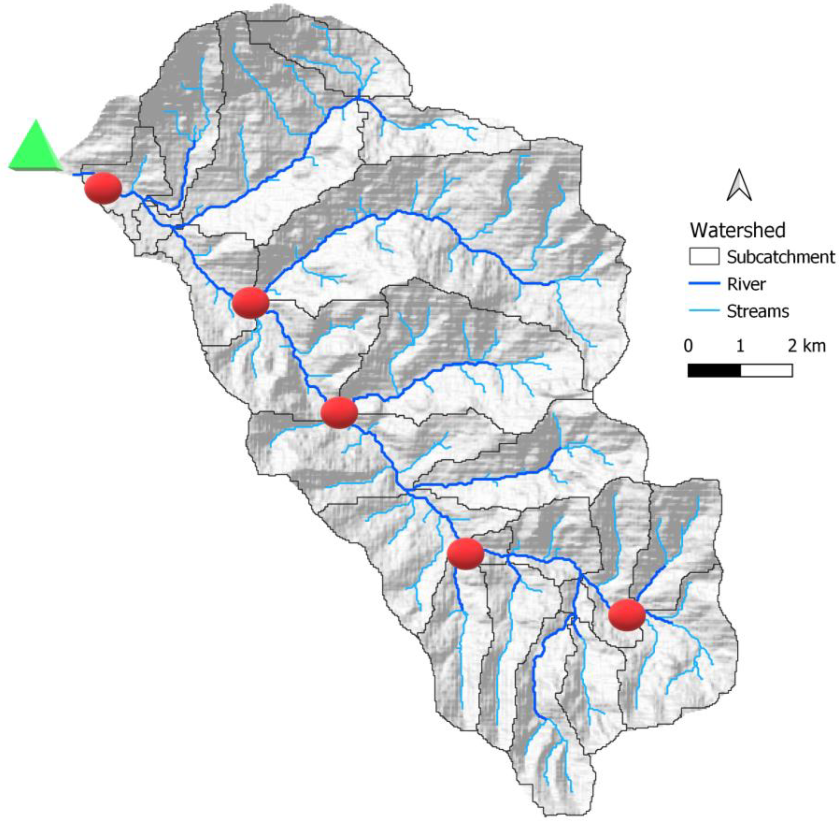
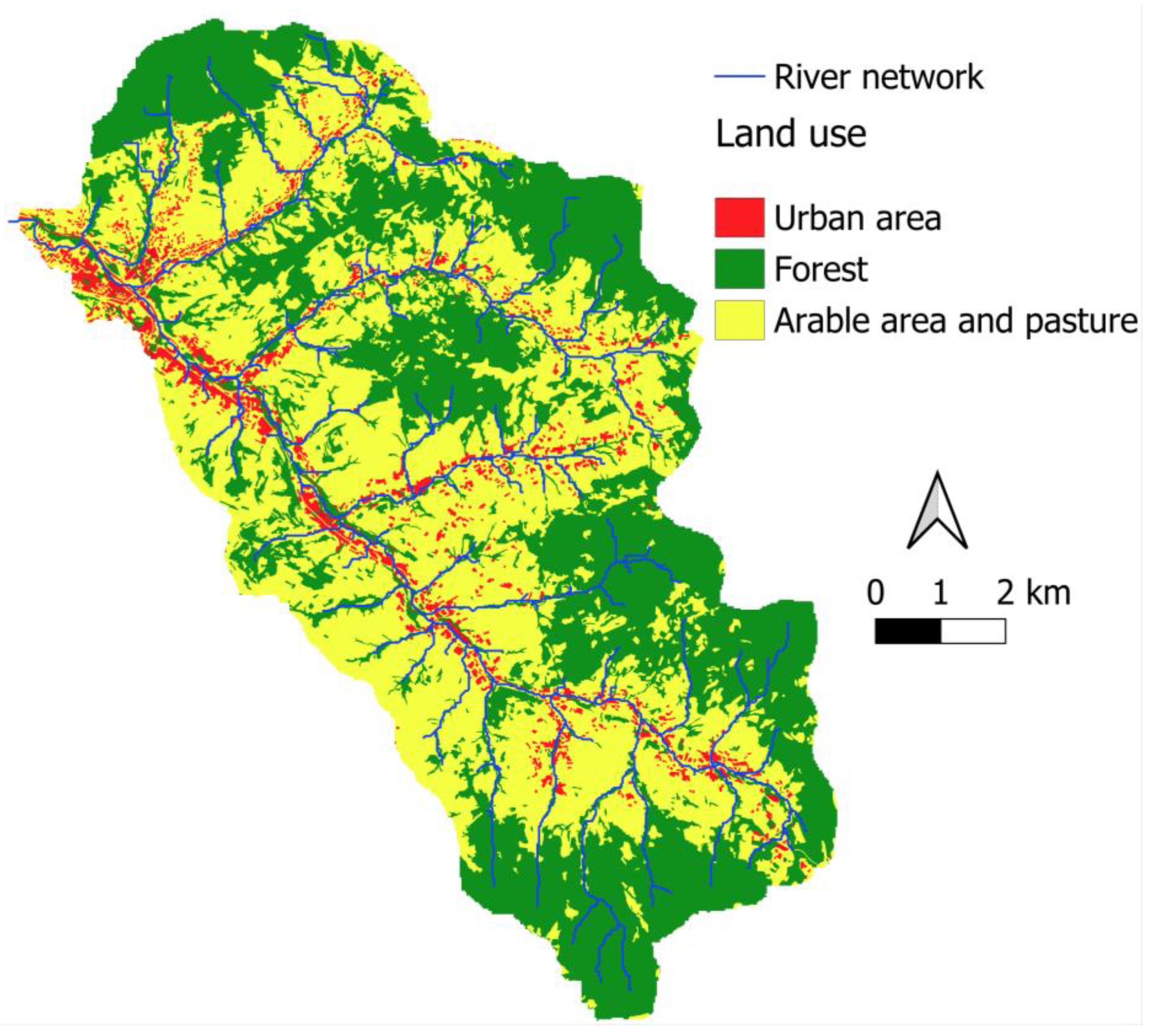
2.1. Research Area

The study area, covering 55 km2, is situated within the Mszanka catchment, a tertiary tributary of the Vistula River and is a part of the Raba River basin in southern Poland (Figure 1). Physico-geographically, it falls under the Carpathian megaregion within the Western Carpathians province [20]. The measurement series was conducted according to the map presented on Figure A1. The terrain is predominantly mountainous and utilized for agriculture and forestry (Figure A2). At lower elevations, European hornbeam forests dominate, while at higher elevations, spruce–fir and fir–juniper forests prevail. Mixed deciduous forests are found in the grazing pastures and permanent grasslands throughout the entire catchment. The map of soil types is located on Figure A4.
The altitude ranges from 371 to 1274 m above sea level. In the Köppen climate classification, the Western Carpathians typically falls under the Dfb climate category. This classification indicates a warm-summer humid continental climate, characterized by average temperatures above 10 °C during the warmest month and at least one month with temperatures below 0 °C. In higher elevation areas, the climate classification may shift to Dfc. The region benefits from abundant water resources primarily due to substantial atmospheric precipitation, with average rainfall ranging from 950 to 1250 mm annually and averaging around 1100 mm. Additionally, temperatures typically range between 6.5 and 8 degrees Celsius. In forested areas, the CN values fall between 71 and 77; in pasture areas, they range from 76 to 82; on arable land, they range from 81 to 91; and in river valleys, the CN value is 98.
The Western Carpathians area traditionally supports pastoral activities. There is now a shift towards sustainable grassland and pasture land use aligned with EU policies, which emphasize improved nutrient management in pastoral systems.

2.2. Physical–Chemical Analyses

Ammonium, nitrate, nitrite, and phosphate were determined by a flow (injection) colorimetric analysis on a computer-controlled FOSS FIAStar 5000 apparatus. NH4+, NO2, NO3, and PO43− were determined and recalculated using a spectrophotometer. NH4+, NO2, NO3, and P-PO43+ Samples from the mountain streams were collected monthly using the bathometric method (containers with a volume of 1 dm3). The concentration of the total suspended solids (TSS) was determined via the gravimetric method (after drying) using tarred filters (with an accuracy of ±0.0005 g). The dry residue (sum of mineral particles from the transported samples) from the collected material was filtered with the filtration method in order to determine the concentration. The total number of water samples was 140 in the period of five years from April to November in each year. A one-month period for sampling is appropriate for water management and grassland use because it captures seasonal variability, balances data sufficiency with resource efficiency, and aligns with regulatory requirements. Monthly sampling is manageable in terms of time, labor, and cost, and it provides enough data to identify trends and inform management decisions, such as irrigation, fertilization, and grazing practices. This frequency also allows for timely detection and mitigation of potential environmental impacts, optimizing resource use and environmental protection.

2.3. Hydrodynamic Measurements

The shear velocity in the stream (u) was calculated using the following formula [21]:
u = h · g · S
where
u—shear velocity (m∙s−1);
h—average water depth (m);
g—gravitational acceleration (m∙s−2);
S—channel bed slope (%).
Hydrodynamic measurements were conducted with a VALEPORT Model 801 Flat EM Flow Meter, which measures the average velocity at intervals of time. The device provides an accuracy of approximately 0.01 m·s−1. In the case of shallow water below 0.3 m, three measurement series were taken. If the water was up to 1 m, it was measured in series. Using the diagrams of velocity distribution above the bottom in a semilogarithmic system, dynamic velocity was calculated, based on the maximum and instantaneous velocities (measured just above the bottom) [22]:
V = a 5.75
where
a—line slope coefficient V = f (h) with the equation y = ax + b (where x—height above the bottom on which the velocity measurement (m∙s−1) was made, b—intercept of the equation) [21]:
D t , y = 0.6 · h · u
where
(Dt, y)—turbulent diffusion coefficient for transverse mixing in the cross-section (m2·s−1);
h—average water depth (m);
u—shear velocity (m·s−1).
The study period coincided with the sampling period described earlier, as both hydrometric and hydrochemical measurements were conducted at identical locations. Flow parameter estimation across the stream was derived from the average of three measurements per cross-section. Measurements were taken at tachymetric points along the stream width. Monthly data series were averaged over the course of one month. Points close to adjacent areas with different land uses were specifically analyzed to determine the influence of these areas on nutrient leaching.

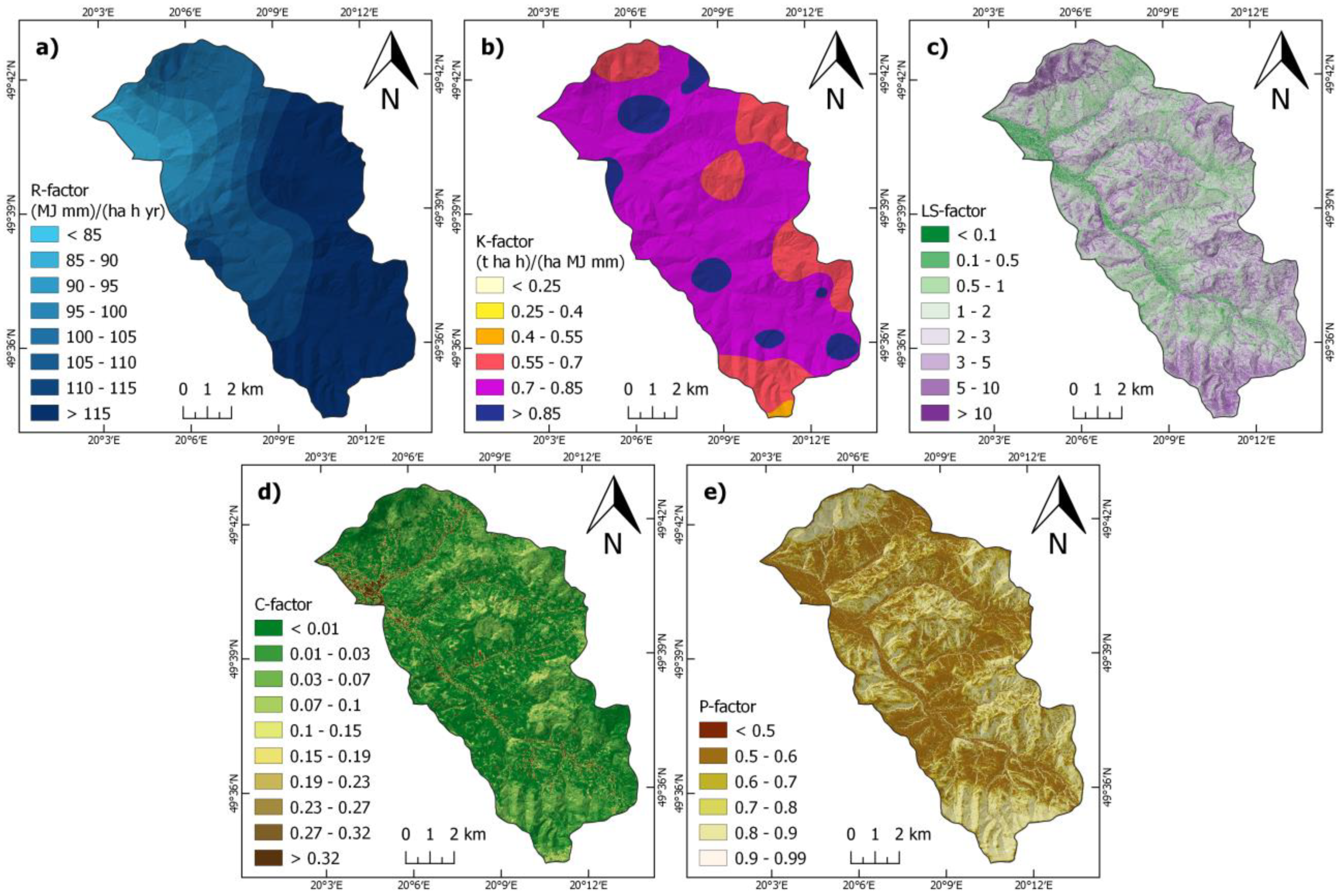
2.4. Hydrological and Soil Erosion Modeling

SWAT+ is a multidimensional (deterministic) physical model capable of calculating various components within a watershed using an extensive set of input parameters. It is designed for small-watershed to river-basin-scale simulations to assess surface water quality. For catchment, we prepared a digital elevation model (DEM) with a resolution of 10 m. For SWAT model input data, we required a DEM, land use, and soil maps. Once the model is prepared in the software, various hydrological processes such as water flow and nutrient flux can be analyzed. SWAT simulates agricultural chemical yields in watersheds to demonstrate the impact of land management practices on water and sediment. We select output data such as nutrient and TSS concentrations to illustrate the erosion outcomes from permanent grasslands, agricultural use, and forests, showcasing the erosive effects on stream water. Using the DEM, we delineated watercourses and subcatchments from raster data. Meteorological data, including daily precipitation, air temperature, solar radiation, and wind speed, were obtained from the Institute of Meteorology and Water Management in Warsaw. The CORINE Land Cover 2018 dataset was used to incorporate land use data into the GIS layers of the model. Subsequently, QGIS version 3.16 was employed to create detailed soil and agricultural maps. All steps involved in creating the model based on input data were followed using QSWAT+, which includes built-in updates added to QGIS, a freely available software. In this study, we utilized subcatchments to analyze input data for water management
The Sequential Uncertainty Fitting (SUFI2) procedure was then applied to calibrate the SWAT+ model using multiannual meteorological data from 1991 to 2020. A SWATplus-CUP with SWAT+ Toolbox was utilized as a calibration parameter for this process. The optimal model variables were selected based on data measured only in the main stream at the five gauge cross-section stations within the study period of 2014–2018. The calibration was conducted for 2014–2016, and validation was performed during 2017–2018. The results were visualized on maps to illustrate the model’s performance. The primary parameter utilized in our study is GE (Kling–Gupta efficiency), which serves as a metric for assessing the performance of hydrological models. This metric is founded on three key components: correlation, bias, and variability.
The KGE metric spans from −∞ to 1, where a value of 1 indicates perfect agreement between the model predictions and the observed data. Additionally, we employed the R2 coefficient of determination to validate the data. Furthermore, we utilized PIAS (Parameter Identification and Sensitivity Analysis), a tool designed for the calibration and analysis of hydrological models. The objective of employing PIAS was to determine the optimal parameter values and to quantify the uncertainty inherent in the model outputs. The calibration and validation processes included the following parameters: TSS, N-NO3, N-NO2, N-NH4+, P-PO43−. The R2 values for simulated and measured values were low and negative at the individual cross-section level. Moreover, it was decided that the values would be verified using R2 for the entire catchment collectively during the study period.
We applied the RUSLE model (Figure A3) to assess erosion across the entire catchment area [23]. During SWAT modeling, we carefully selected the main streams and tributaries for the calibration process. Subsequently, we categorized the catchment into three distinct land uses: forest, arable land, and pasture. Based on an understanding of vegetation succession, the classification of land use was categorized into distinct types. Forests were delineated where tree species dominated the landscape, arable land was designated for agricultural cultivation activities, and pastures were identified as areas utilized for livestock grazing. These categories were chosen for spatial regression analysis focusing on nutrient leaching.

2.5. Spatial Analysis

The relation between the turbulent diffusion index and inorganic nutrients and TSS (physicochemical indices) randomly distributed in the surface water was studied using spatial autoregression (SAR) with a lagged response model [24]:
Y = ρ·Wy + + ε
where
Y—responsive (explained) variable;
Wy—the spatial lag of Y, which is the weighted average of neighboring Y values;
ρ—spatial interaction coefficient (spatial autoregression parameter reflecting the relationship between the variables);
X—a matrix of independent variables;
β—a vector of coefficients associated with the independent variables;
ε—the random component (error of spatial estimation not described by the model; random effect).
We categorized the catchment into three distinct land uses: forest, arable land, and pastures. At the water sampling sites where alterations in land use were observed and physical properties were measured, we applied spatial autoregressive (SAR) models to analyze the spatial dynamics. We also checked for nutrient leaching. We assumed that the points close to adjacent areas are connected with the leaching. Spatial regression in space and time should show the interconnection. Spatial autoregression (SAR) models are statistical techniques used to analyze spatial data, accounting for spatial dependence or autocorrelation. By regressing variables at one location on those at neighboring locations, SAR models capture spatial dependency and enable an examination of how changes in one area affect nearby locations. This nuanced understanding is crucial for studying complex spatial phenomena. In catchment applications, SAR modeling involves several critical stages, including data collection, preprocessing, construction of a spatial weight matrix, model customization, parameter estimation, model assessment, and interpretation. These steps facilitate accurate analyses and uncover relationships between variables and spatial dependencies within the catchment.

3. Results

3.1. Inorganic Nutrients and TSS Concentrations

The concentration of ammonium was relatively consistent across all cross-sections, ranging from 0.81 mg/dm3 to 0.97 mg/dm3. The concentration rises sharply from 0.10 mg/dm3 at cross-section 2 to 0.61 mg/dm3 at cross-section 5. The concentration of nitrate increases significantly from cross-section 1 (0.72 mg/dm3) to cross-section 5 (1.89 mg/dm3). The highest increase was observed between cross-section 4 (0.24 mg/dm3) and cross-section 5 (0.32 mg/dm3). The average flow ranged from 0.68 to 1.96 m3/s depending on the measurement cross-section. The concentration of TSS showed an increase from cross-section 1 to cross-section 5 (Table 1).

3.2. Hydrodynamic Appraisal

For both flysch streams, the calculated transport intensity was found in the water in the part of the catchment used for agriculture. The transverse turbulence diffusion coefficients did not differ. On average, 0.094 m2·s−1 of water was adjacent to arable land in the main stream. Water in both streams that were predominantly surrounded by arable land was mixed with hydrochemical indicators after a distance of 50 m (Table 2).

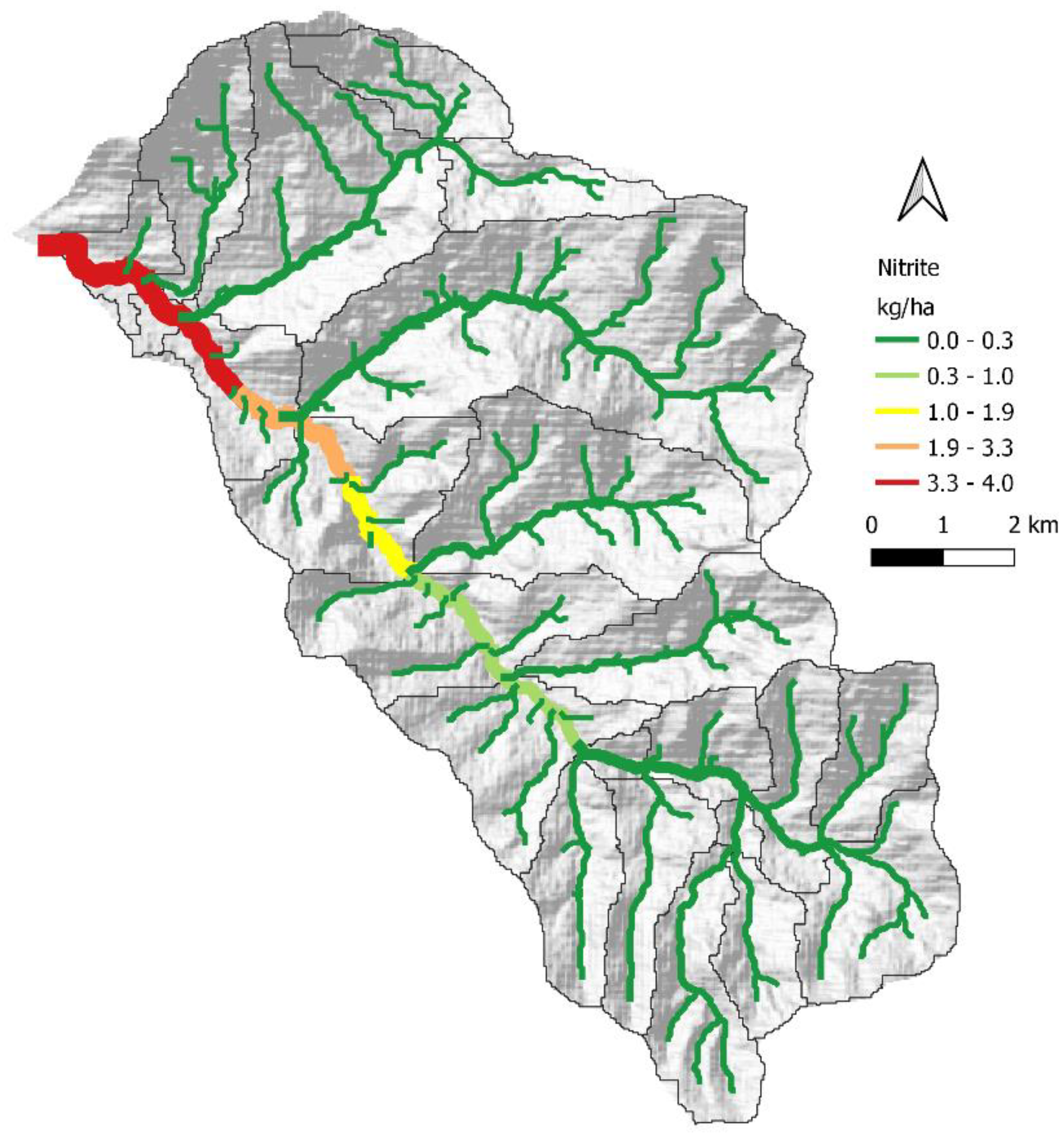
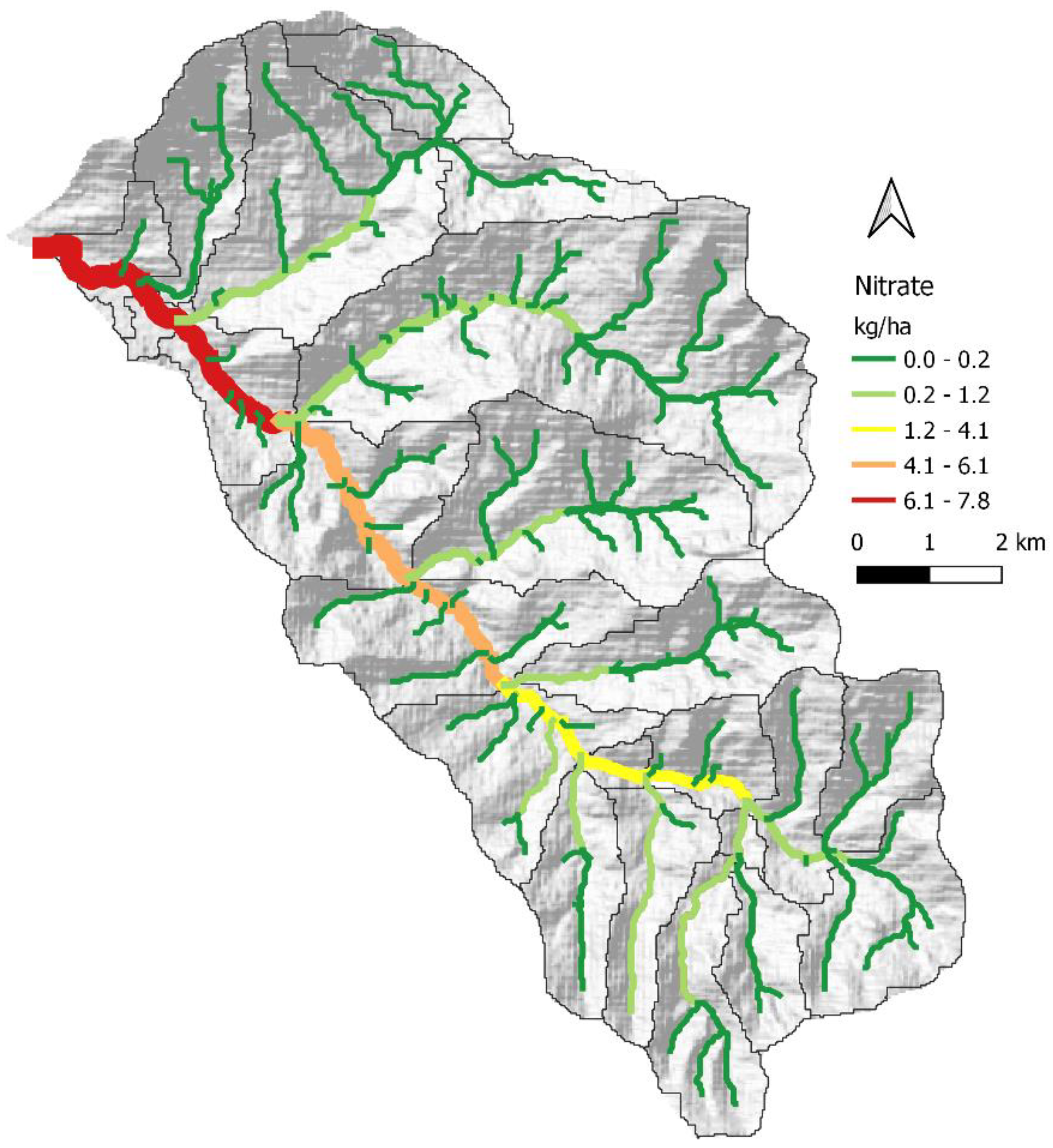
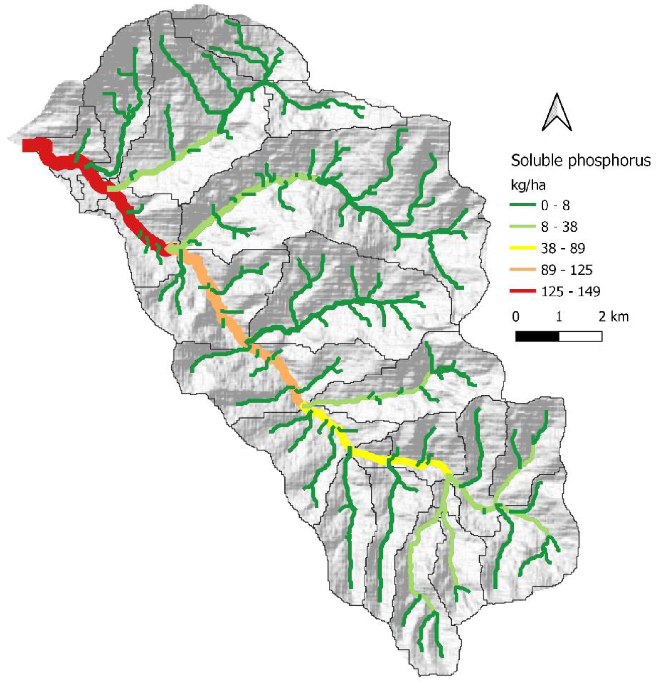
3.3. Spatial In-Stream Inorganic Nutrients and TSS Modeling

Autoregression analysis (SAR) showed the spatial relationship between arable land and selected water quality indicators, especially N-NO3- and TSS for the Mszanka stream (Table 3). SAR showed a statistically significant spatial relationship between permanent grasslands and the water of the stream for P-PO43− and TSS (Table 4). The forested part of the catchment area showed significant spatial relationships to the N-NO3 concentration in the water.
The daily ammonium concentration ranged from 0.1 to 3.6 kg/ha (Figure 2). The nitrite concentration in the main drainage watercourse peaked at 4 kg/ha at the outlet (Figure 3). The nitrate concentration in the main drainage watercourse was also highest at the outlet, with a daily value of 7.8 kg/ha (Figure 4). The phosphorus concentration reached a maximum of 149 kg/ha at the outlet (Figure 4). The TSS was highest in the tributaries, ranging from 410 to 580 kg/ha daily (Figure 5). The RUSLE model showed that mountainous areas had the highest erosion rates, exceeding 50 t/ha/year, while pasture areas had the lowest erosion rates, between 0.5 t/ha/year (Figure 6).
Sequentially, for the waters of the Mszanka stream, phosphorus phosphate ranged from 0.09–0.34 mg·dm−3 (Table 1). Spatial autoregression analysis demonstrated interrelations between P-PO43− concentrations and pastures in the main stream (Table 5).
This is particularly evident on sections with large slopes in the upper part of the subcatchments. In the main drainage watercourse, the modeled phosphate phosphorus values ranged from 125 to 149 kg/ha (Figure 4). The modeled values for the total suspended sediment fluctuated from 0.01 to 580 kg/ha (Figure 5).
Calibration and validation revealed that N-NO3 was the most suitable for catchment; the key parameters were flow and TSS (Table 6).

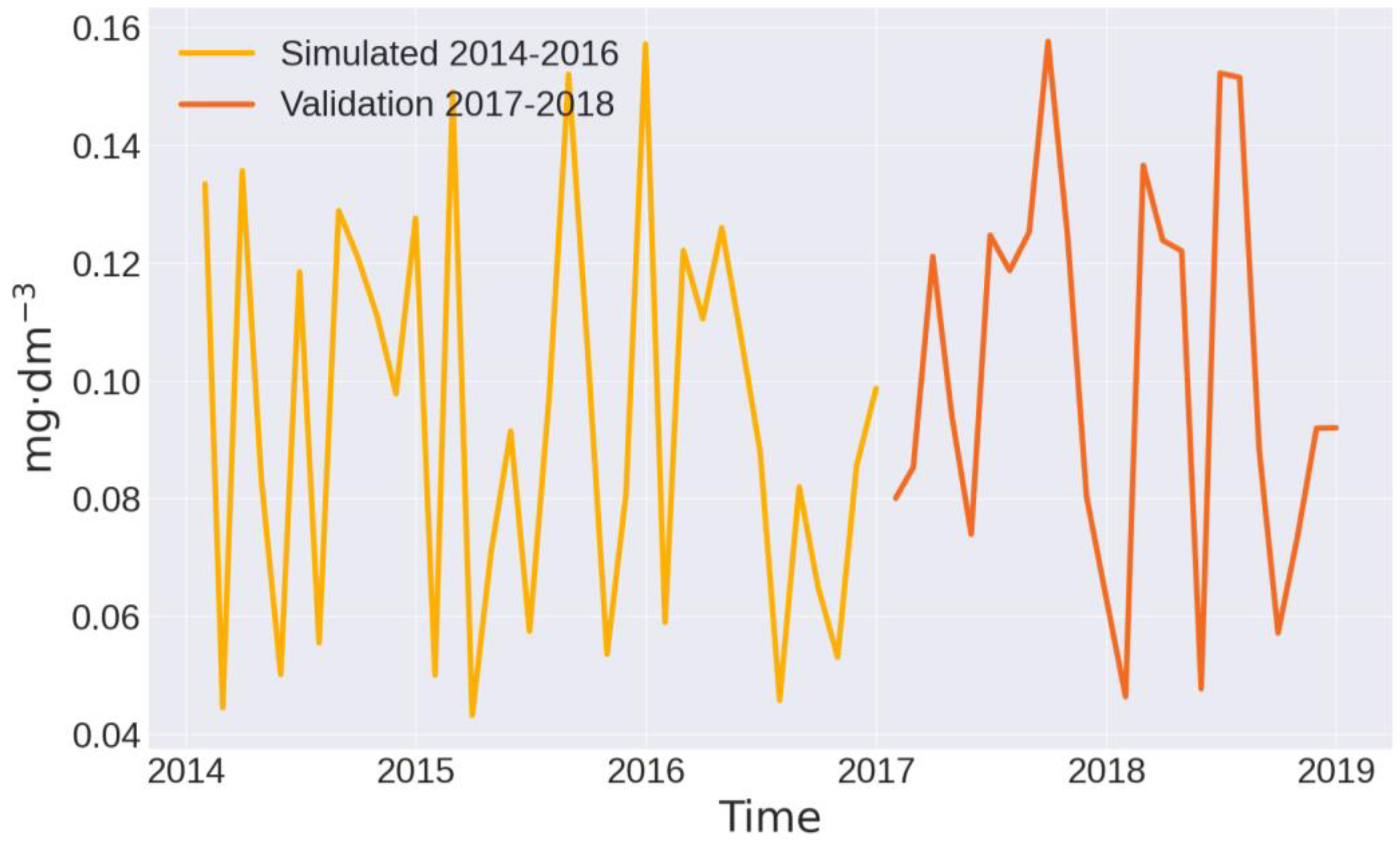
3.4. Model Performance in the Main Stream

The simulated ammonium concentrations closely matched the observed data during both the calibration and validation periods. This indicates that the model accurately captured the spatial and temporal dynamics of ammonium leaching in the catchment area (Figure A5). The nitrite concentrations showed a reasonable match between simulated and observed data, with slight deviations during peak events (Figure A6). Nitrate levels demonstrated good agreement between simulation and observed data, especially during the calibration period. There were minor discrepancies during the validation period, likely due to changing land use practices or climatic variations (Figure A7). Phosphate levels in the simulation were consistent with observed data, though there were occasional overestimations during the validation period (Figure A8). Criteria for selecting input data for nutrient simulation are described in Table 7. The simulated TSS values closely followed the observed data trends, capturing both base flow and peak flow conditions accurately (Figure A9).

4. Discussion

4.1. Examination of Land Use on TSS Leaching and Inorganic Nutrient Concentrations

In recent years, watershed modelers have put increasing emphasis on simulating watershed processes as realistically as possible [25,26]. For the correct diagnosis of agricultural production in the hilly terrain, predictions of erosion losses are crucial [27,28]. By using the catchment area effectively, water quality can be improved [29,30,31]. A large effect is related to the way the adjacent area has been used and developed. In forest areas, in small mountain catchments, land changes are less pronounced [32]. The system of tributaries to the main watercourse dominated by forest land maximizes this effect.
There was an increase in concentrations of nitrite, nitrate, phosphorus, phosphate, and from upstream to downstream cross-sections. The highest discharge was recorded at the outlet of the studied stream (Table 1), indicating that water accumulates more nutrients and suspended solids as it flows downstream. The relatively stable concentration of ammonium across the cross-sections suggests that ammonium levels are not significantly influenced by downstream flow or additional sources of contamination. The substantial increases in nitrate and phosphate concentrations suggest potential agricultural runoff or other nutrient sources entering the water body downstream, contributing to higher nutrient loads. The sharp rise in TSS in the upstream sections, particularly at cross-section 1, may be attributed to increased erosion, runoff, or other sources introducing suspended particles into the stream. The high TSS levels in the upstream areas were confirmed by soil erosion, as shown in Figure 7, which utilized the Revised Universal Soil Loss Equation (RUSLE) model for catchment. In other locations where high surface erosion rates were noted, protective water retention measures and practices, such as the use of vegetative buffer zones, could be observed. This demonstrates that agricultural land use can either increase or decrease soil erosion and loss, emphasizing the importance of choosing methods carefully and highlighting variations in agricultural practices.
Spatial autoregression has revaluated that interrelation. Permanent grasslands limit the supply of weathered material (Table 5). Prognostic models for the Mątny stream catchment area near Gorce and Beskid Wyspowy showed that potato crops were most susceptible to soil erosion [33]. As forests slow soil erosion, they are an important source of protection against water erosion [34]. The methods employed to assess the intensity of water erosion are shaped by contemporary morphogenetic processes. It should be mentioned that, additionally, the physiographic features of the catchment area play a major role in determining soil losses [35].
The leaching effect of inorganic nutrients can be mitigated by enhanced vegetation cover. As evidenced by the findings, areas with permanent grasslands exhibited the lowest levels of inorganic nutrient loss. Furthermore, while the tributaries showed low concentrations of the studied inorganic nutrients, their concentration in the main stream progressively rises. The model’s ability to predict TSS levels suggests its reliability in simulating erosion and sediment transport processes within the catchment (Figure A9).

4.2. Transport of Inorganic Nutrients and TSS Floating in the Watercourse

It is also common to find mechanisms of transport of sedimentary materials related to clastic weathering of the soil [36]. Consequently, in the mountain area, denudation mechanisms may be easily estimated [37] for N-NO3 [38]. Small catchments are subject to slow chemical denudation and a smaller size of rinsed weathered drainage than channel processes, where the sedimentation rate and nitrate flux of fluvial material changes with the flow of water [39]. For the studied stream, it is almost 6.5–7.8 kg/ha (Figure 3). The model effectively captured general trends in nitrite levels, though further refinement may be needed for extreme conditions. This suggests that the model can be used for general predictions but should be cautiously applied for extreme event analysis (Figure A6). The model is robust in predicting nitrate concentrations (Figure A7), making it useful for planning and management decisions aimed at reducing nitrate leaching. Other forms of nitrogen were distributed similarly; the highest flow rate results in greater leaching to the main watercourses (Figure 1 and Figure 2). In the main watercourse, we observed a gradual decrease in TSS concentration the closer to the outlet (Figure 6). This may be due to the hydromorphological parameters and the reduction in the flow velocity, which favors the sedimentation and hydrodynamic process [40]. This study, using the hydrological model, showed that ammoniacal nitrogen is concentrated mainly in the outlet drainage area (Figure 2). The SWAT+ model also demonstrated that nitrate nitrogen (Figure 4) accumulated especially in the main stream. Additionally, we observed similar concentrations of phosphate in the outlet of the main stream (Figure 5). The slight overestimations indicated that while the model is effective, it might benefit from additional calibration to account for specific land management practices that affect phosphate phosphorus leaching (Figure A8).
There should be a method developed to depict the full transport path of clastic material in order to visualize the relationship between the total suspended solid content and the characteristics of surface water quality. The sources of pollution and the scale of the risk of water and surface erosion should be considered. Hazard assessments of transported clastic weathering are needed for surface water protection plans [41] and environmental requirements related to soil conservation [42]. Meanwhile, in the Western Carpathian mountains, such systems are also used for forecasting landslide risks and for applying fertilizers in agricultural areas. With the SWAT+ model, it was observed that leaching in the streams at the catchment’s outlet was highly concentrated, especially by nitrate in the outlet of the main stream (Figure 3). In a subsequent study, the daily concentration of total suspended sediment (TSS) should be compared with the monthly precipitation totals in a given year in order to determine the intensity of erosion. It was also indirectly demonstrated that, regardless of the scale of the flysch catchment, the leaching tendency of inorganic nutrient compounds was maintained. The key factors were the land use of the catchment area and the density of the hydrographic network, especially the flow of the river.

4.3. Applications of SWAT + Model in the Aspect of Precipitation

While the Beskidy streams’ landscape undergoes periodic weathering, the quantity of material discharged and accumulated does not align proportionally with the flow [43]. The erosive impact of rainwater actively degrades soil by forcefully carrying away its material, driven by the intensity of the rainfall [44]. According to Martínez-Mena et al. (2020), soil vulnerability to erosion and surface runoff is contingent upon granulometry, water absorption (water accumulation), permeability, and hydrogeology. Following a severe rainfall event with at least 100 mm/h intensity, a targeted, vigorous surface wash occurs. Interestingly, a mere 20 mm of daily rainfall serves as a threshold, initiating initial soil washing in a small catchment [45]. The extended heavy rains, accumulating a precipitation sum of 50 to 150 mm over several days, intensify both hydrological and geomorphological processes. This, in turn, induces fine-scale surface erosion [43]. A portion of the rainfall infiltrates the ground through percolation as an aqueous solution, while the rest flows along the stream, carrying soil particles with it. As a result, there is a noticeable increase in the accumulation of soluble forms of inorganic nutrients in the main watercourse (Figure 4). Effective calibration parameters and model setup contributed to the accurate prediction of ammonium levels (Figure A5), reflecting the impact of land use and agricultural practices. Roughness of the nitrate runoff loss from intensive farmland determines water storage on the soil surface and may indirectly affect its ability for infiltration and risk of nitrate leaching [46,47]. Rough surfaces increase hydraulic resistance, which allows weathered soil to be carried by rainwater flowing down an incline [48]. A solation mechanism propels aggregates less than 0.05 mm. As the intensity of water erosion increases, the relationship between erosion forces and sediment load changes [49]. A change in the roughness of the soil surface occurs at a precipitation intensity of 0.68 mm∙min−1. Then, soil particles migrate along the slope as the size of splash erosion increases [50,51]. For each catchment, TSS is spatially distributed in tributaries differently. There is no accumulation of TSS concentration in the main watercourse following its outflow. Neither the catchment area nor the density of the hydrographic network contributes to differences in the concentration of TSS. The TSS fluxes are triggered by this process. Similarly, the forested part of catchments influences the TSS leaching process (Figure 5). In a scenario where no changes in land use are implemented, a study of the Grajcarek stream, located in the Lesser Pieniny mountains in the Polish Carpathians, uncovered an average annual loss of topsoil (average upland sediment yield) amounting to 14.3 Mg∙ha−1. The maximum upland sediment yield in this scenario peaked at 94.6 Mg∙ha−1. Notably, there was a significant accumulation of soil material in the lower part of the catchment, resulting in an average in-stream sediment change of 13.27 Mg∙ha−1 per year [52]. This suggests that management in rich-relief flysch catchments should be geared towards the forest. Accordingly, the studied river valleys do not possess the capacity of retaining inorganic nutrient forms, while in the case of TSS, this may result in earlier sedimentation in the river channel [53]. One of the primary mechanisms influencing this process is the erosion of soil particles. The state of water quality in the catchment is crucial for understanding implications for land and agricultural water management [54,55,56,57,58,59]. In this study, a QSWAT+ model was developed to thoroughly analyze the distribution of phosphorus and nitrogen concentrations in mountain streams, particularly within agricultural areas. The integration of both passive and active output data has proven crucial in addressing knowledge gaps within the surface water sector. Incorporating remote sensing data is highly recommended for researchers, as it significantly enhances our ability to achieve a nuanced and comprehensive understanding of the obtained results, extending to other water bodies such as rivers, lakes, reservoirs, and wetlands.

5. Conclusions

The interplay of nutrient management is crucial for accurately understanding the physical characteristics of watersheds and has significant implications for agricultural management. This research utilizes an extensively refined version of the SWAT+ model and associated techniques to capture variations in river discharge, sediment yield, and nutrient flow. In the agricultural arable section of the watershed, we noted a higher leaching of inorganic compounds compared to areas occupied by pastures and forests. These objectives collectively seek to enhance our understanding of inorganic nutrient dynamics and the dispersion of total suspended solids (TSS) within a pasture-dominated catchment influenced by water erosion. This understanding will contribute to strategies aimed at reducing nitrogen and phosphorus levels in the historically intensely exploited agricultural areas of the Western Carpathians, underscoring the significant influence of human activity on water quality dynamics. The hydrological model can assist in maintaining appropriate vegetative cover and implementing management strategies for pasture lands to mitigate fluctuations in inorganic nutrient concentrations and TSS. Surprisingly, TSS concentrations in waterways were minimally affected by anthropogenic land use compared to inorganic nutrients. Instead, areas with high TSS tend to accumulate sediment, suggesting lower susceptibility to leaching in the vegetated parts of the catchments, such as pasture and forest zones. Data from pasture land use support these findings, emphasizing the need for thorough maintenance of vegetation in this agricultural system. Future studies should explore other nutrient forms and pollutants across diverse landscapes and agricultural systems, especially in mountainous regions. Findings from cross-sectional turbulence coefficient analysis reveal heightened TSS and inorganic nutrient fluxes in the main streams studied. Noteworthy is the observation that watershed areas tend to accumulate TSS in various subcatchments, displaying lower susceptibility to leaching. Conversely, in river-based scale analyses, surface runoff emerges as the predominant influencer of inorganic nutrient concentrations. For researchers aiming to make comparisons among datasets, maintaining comprehensive records of data types, processing methodologies, and resultant findings from this application is recommended. Future studies are encouraged to consider other nutrient forms (e.g., organic) or pollutants on a broader spatial scale, particularly in mountainous regions.

Author Contributions

Conceptualization, W.H.; methodology, W.H. and D.B.; software, W.H.; validation, W.H.; formal analysis D.B. All authors have read and agreed to the published version of the manuscript.

Funding

This research was funded by the Ministry of Science and Higher Education for University of Agriculture in Krakow in 2024 year.

Data Availability Statement

Data are available on request.

Conflicts of Interest

The authors declare no conflicts of interest.

Appendix A

Figure A1. The location of monitored cross-sections in the stream network. Cross-sections with control stations are marked with red dots. The green triangle indicates the location of the meteorological observation post for measurement.
Water 16 02052 g0a1
Figure A2. Land use of studied catchment.
Water 16 02052 g0a2
Figure A3. Parameters of RUSLE model. R is the rainfall-runoff erosivity factor, K is the soil erodibility factor, LS is the slope length and the slope steepness factor, C is the land cover and management factor, P is the soil conservation or prevention practices factor.
Water 16 02052 g0a3
Figure A4. Soil type map for investigate catchment.
Water 16 02052 g0a4
Figure A5. Simulated and validated data for N-NH4 in the main stream.
Water 16 02052 g0a5
Figure A6. Simulated and validated data for N-NO2 in the main stream.
Water 16 02052 g0a6
Figure A7. Simulated and validated data for N-NO3 in the main stream.
Water 16 02052 g0a7
Figure A8. Simulated and validated data for P-PO43− in the main stream.
Water 16 02052 g0a8
Figure A9. Simulated and validated data for TSS in the main stream.
Water 16 02052 g0a9

References

  1. Centanni, M.; Ricci, G.F.; De Girolamo, A.M.; Gentile, F. Modeling pesticides and ecotoxicological risk assessment in an intermittent river using SWAT. Sci. Rep. 2024, 14, 6389. [Google Scholar] [CrossRef]
  2. Bärlund, I.; Kirkkala, T.; Malve, O.; Kämäri, J. Assessing SWAT model performance in the evaluation of management actions for the implementation of the Water Framework Directive in a Finnish catchment. Environ. Model. Softw. 2007, 22, 719–724. [Google Scholar] [CrossRef]
  3. Malagó, A.; Bouraoui, F.; Vigiak, O.; Grizzetti, B.; Pastori, M. Modelling water and nutrient fluxes in the Danube River Basin with SWAT. Sci. Total Environ. 2017, 603, 196–218. [Google Scholar] [CrossRef]
  4. Németová, Z.; Kohnová, S. Mathematical modeling of soil erosion processes using physically-based and empirical models: Case study of Slovakia and central Poland. Acta Hydrol. Slovaca 2021, 22, 147–155. [Google Scholar] [CrossRef]
  5. Akan, C.J.; Abbagambo, M.T.; Chellube, Z.M.; Abdulrahman, F.I. Assessment of Pollutants in Water and Sediment Samples in Lake Chad. Baga, North Eastern Nigeria. J. Environ. Prot. 2012, 3, 1428–1441. [Google Scholar] [CrossRef]
  6. Purandara, B.K.; Varadarajan, N.; Venkatesh, B.; Choubey, V.K. Surface Water Quality Evaluation and Modeling of Ghataprabha River, Karnataka, India. Environ. Monit. Assess. 2012, 184, 1371–1378. [Google Scholar] [CrossRef]
  7. Bedla, D.; Misztal, A. Changeability of Chemistry of Small Water Reservoirs with Diversified Use Structure of the Adjoining Areas. Rocz. Ochr. Srodowiska 2014, 16, 421–439. [Google Scholar]
  8. Halecki, W.; Kowalik, T.; Bogdał, A. Multiannual Assessment of the Risk of Surface Water Erosion and Metal Accumulation Indices in the Flysch Stream Using the MARS Model in the Polish Outer Western Carpathians. Sustainability 2019, 11, 7189. [Google Scholar] [CrossRef]
  9. da Silva, A.M. Rainfall erosivity map of Brazil. Catena 2004, 57, 251–259. [Google Scholar] [CrossRef]
  10. Robson, B. State of the Art in Modelling of Phosphorus in Aquatic Systems: Review, Criticisms and Commentary. Environ. Model Softw. 2014, 61, 339–359. [Google Scholar] [CrossRef]
  11. Brocca, L.; Moramarco, T.; Melone, F.; Wagner, W.; Hasenauer, S.; Hahn, S. Assimilation of surface and root-zone ASCAT soil moisture products into rainfall-runoff modelling. IEEE Trans. Geosci. Remote Sens. 2012, 50, 2542–2555. [Google Scholar] [CrossRef]
  12. Seneviratne, S.I.; Corti, T.; Davin, E.L.; Hirschi, M.; Jaeger, E.B.; Lehner, I.; Orlowsky, B. Investigating Soil Moisture-Climate Interactions in a Changing Climate: A Review. Earth-Sci. Rev. 2010, 99, 125–161. [Google Scholar] [CrossRef]
  13. Kowalczyk, A.; Twardy, S. Wielkość erozji wodnej obliczona metodą USLE. Woda-Sr.-Obsz. Wiej. 2012, 12, 83–92. [Google Scholar]
  14. Vermeulen, H.R.; Nieuwenhuis, J.D. Kinetic Energy Rainfall Relationship for Central Cebu, Philippines for Soil Erosion. J. Hydrol. 2005, 300, 20–32. [Google Scholar]
  15. Mostowik, K.; Krzyczman, D.; Płaczkowska, E.; Rzonca, B.; Siwek, J.; Wacławczyk, P. Spring recharge and groundwater flow patterns in flysch aquifer in the Połonina Wetlińska Massif in the Carpathian Mountains. J. Mt. Sci. 2021, 18, 819–833. [Google Scholar] [CrossRef]
  16. Obi, M.E.; Salako, F.K. Rainfall Parameters Influencing Erosivity in Southeastern Nigeria. Catena 1995, 24, 275–287. [Google Scholar] [CrossRef]
  17. Gil, E.; Kijowska-Strugała, M.; Demczuk, P. Soil erosion dynamics on a cultivated slope in the Western Polish Carpathians based on over 30 years of plot studies. Catena 2021, 207, 105682. [Google Scholar] [CrossRef]
  18. Zhao, Z.; Zhou, Y.; Wang, X.; Wang, Z.; Bai, Y. Water Quality Evolution Mechanism Modeling and Health Risk Assessment Based on Stochastic Hybrid Dynamic Systems. Expert Syst. Appl. 2022, 191, 116404. [Google Scholar] [CrossRef]
  19. Moreno, J.; Campagnolo, L.; Boitier, B.; Nikas, A.; Koasidis, K.; Gambhir, A.; Vielle, M. The Impacts of Decarbonization Pathways on Sustainable Development Goals in the European Union. Commun. Earth Environ. 2024, 5, 136. [Google Scholar] [CrossRef]
  20. Kondracki, J. Geografia Regionalna Polski; Wydawnictwo Naukowe PWN: Wydawnictwo Naukowe PWN, 2011. [Google Scholar]
  21. Loga, M. Wody Pod Presją—Praktyczny Kurs Oceny Presji Obiektów Gospodarki Komunalnej na Wody Powierzchniowe; Praca Zbiorowa: Warszawa, Poland, 2016; ISBN 978-83-937934-4-0. [Google Scholar]
  22. Gordon, N.D.; McMahon, T.A.; Finlayson, B.L.; Gippel, C.J.; Nathan, R.J. Stream Hydrology: An Introduction for Ecologists; John Wiley and Sons: Hoboken, NJ, USA, 2004. [Google Scholar]
  23. Weslati, O.; Serbaji, M.M. Spatial Assessment of Soil Erosion by Water Using RUSLE Model, Remote Sensing and GIS: A Case Study of Mellegue Watershed, Algeria–Tunisia. Environ. Monit. Assess. 2024, 196, 14. [Google Scholar] [CrossRef] [PubMed]
  24. Rangel, T.F.L.V.B.; Diniz-Filho, J.A.F.; Bini, L.M. SAM: A Comprehensive Application for Spatial Analysis in Macroecology. Ecography 2010, 33, 46–50. [Google Scholar] [CrossRef]
  25. Nasirzadehdizaji, R.; Akyüz, D.E. Application of SWAT Hydrological Model to Assess the Impacts of Land Use Change on Sediment Loads. Int. J. Agric. Environ. Food Sci. 2022, 6, 108–120. [Google Scholar] [CrossRef]
  26. Senent-Aparicio, J.; George, C.; Srinivasan, R. Introducing a New Post-Processing Tool for the SWAT+ Model to Evaluate Environmental Flows. Environ. Model Softw. 2021, 136, 104944. [Google Scholar] [CrossRef]
  27. Basha, G.; Ouarda, T.B.M.J.; Marpu, P.R. Long-term projections of temperature, precipitation and soil moisture using non-stationary oscillation processes over the UAE region. Int. J. Climatol. 2015, 35, 4606–4618. [Google Scholar] [CrossRef]
  28. Smoroń, S.; Kowalczyk, A.; Kostuch, M. Użytkowanie Gruntów Zlewni Szreniawy w Kontekście Ochrony Gleby i Wody w Latach 1995–2005. Woda-Sr.-Obsz. Wiej. 2009, 9, 167–179. [Google Scholar]
  29. Abeysingha, N.S.; Singh, M.; Sehgal, V.K.; Khanna, M.; Pathak, H.; Jayakody, P.; Srinivasan, R. Assessment of water yield and evapotranspiration over 1985 to 2010 in the Gomti River basin in India using the SWAT model. Curr. Sci. 2015, 108, 2202–2212. [Google Scholar]
  30. Bedla, D.; Król, K. The impact of land use on water quality in rural pond on the example of the pond Zelków. Acta Sci. Polonorum. Form. Circumiectus 2014, 13, 25. [Google Scholar] [CrossRef]
  31. Luis, A.T.; Teixeira, P.; Almeida, S.F.; Matos, J.X.; da Silva, E.F. Environmental impact of mining activities in the Lousal area (Portugal): Chemical and diatom characterization of metal contaminated stream sediments and surface water of Corona stream. Sci. Total Environ. 2011, 409, 4312–4325. [Google Scholar] [CrossRef]
  32. Woo, S.Y.; Kim, S.J.; Lee, J.W.; Kim, S.H.; Kim, Y.W. Evaluating the Impact of Interbasin Water Transfer on Water Quality in the Recipient River Basin with SWAT. Sci. Total Environ. 2021, 776, 145984. [Google Scholar] [CrossRef]
  33. Halecki, W.; Kruk, E.; Ryczek, M. Evaluation of water erosion at a mountain catchment in Poland using the G2 model. Catena 2018, 164, 116–124. [Google Scholar] [CrossRef]
  34. Stępniewski, K.; Demczuk, P.; Rodzik, J.; Siwek, K. Związki Między Opadem Deszczu a Spływem Powierzchniowym i Spłukiwaniem Gleby na Poletkach Doświadczalnych o Różnym Użytkowaniu (Guciów—Roztocze Środkowe). Pract. Stud. Geogr. 2010, 45, 229–241. [Google Scholar]
  35. Halecki, W.; Kruk, E.; Ryczek, M. Estimations of nitrate nitrogen, total phosphorus flux and suspended sediment concentration (SSC) as indicators of surface-erosion processes using an ANN (Artificial Neural Network) based on geomorphological parameters in mountainous catchments. Ecol. Indic. 2018, 91C, 461–469. [Google Scholar] [CrossRef]
  36. Łach, J. Rola Gwałtownych Ulew i Powodzi w Modelowaniu Rzeźby Kotliny Kłodzkiej oraz Zachodnich Pasm Górskich Sudetów Wschodnich; Instytut Geografii i Rozwoju Regionalnego UW: Wrocław, Poland, 2012. [Google Scholar]
  37. Baryła, A. 2004. Erozyjność deszczy w rejonie Puczniewa. Przeg. Nauk. Inżynierii Kształtowania Sr. 2004, 13, 48–54. [Google Scholar]
  38. Wu, S.; Tetzlaff, D.; Goldhammer, T.; Soulsby, C. Hydroclimatic Variability and Riparian Wetland Restoration Control the Hydrology and Nutrient Fluxes in a Lowland Agricultural Catchment. J. Hydrol. 2021, 603, 126904. [Google Scholar] [CrossRef]
  39. Richards, G.; Gilmore, T.E.; Mittelstet, A.R.; Messer, T.L.; Snow, D.D. Baseflow Nitrate Dynamics within Nested Watersheds of an Agricultural Stream in Nebraska, USA. Agric. Ecosyst. Environ. 2021, 308, 107223. [Google Scholar] [CrossRef]
  40. Wu, S.; Tetzlaff, D.; Yang, X.; Soulsby, C. Disentangling the Influence of Landscape Characteristics, Hydroclimatic Variability and Land Management on Surface Water NO3-N Dynamics: Spatially Distributed Modeling Over 30 yr in a Lowland Mixed Land Use Catchment. Water Resour. Res. 2022, 58, e2021WR030566. [Google Scholar] [CrossRef]
  41. Haritash, A.K.; Gaur, S.; Garg, S. Assessment of water quality and suitability analysis of River Ganga in Rishikesh, India. Appl. Water Sci. 2016, 6, 383–392. [Google Scholar] [CrossRef]
  42. Barbayiannis, N.; Panayotopoulos, K.; Psaltopoulos, D.; Skuras, D. The influence of policy on soil conservation: A case study from Greece. Land Degrad. Dev. 2011, 22, 47–57. [Google Scholar] [CrossRef]
  43. Starkel, L. Geomorphic Hazards in the Polish Flysch Carpathians. Stud. Geomorphol. Carpatho-Balc. 2006, 40, 7–19. [Google Scholar]
  44. Meusburger, K.; Steel, A.; Panagos, P.; Montanarella, L.; Alewell, C. Spatial and temporal variability of rainfall erosivity factor for Switzerland. Hydrol. Earth Syst. Sci. 2012, 16, 167–177. [Google Scholar] [CrossRef]
  45. Kruk, E. Influence of daily precipitation on yield of eroded soil in mountain basin using the MUSLE model. Acta Sci. Pol. Form. Circumiectus 2017, 16, 147–158. [Google Scholar] [CrossRef]
  46. Lin, B.; Chen, X.; Yao, H.; Chen, Y.; Liu, M.; Gao, L.; James, A. Analyses of landuse change impacts on catchment runoff using different time indicators based on SWAT model. Ecol. Indic. 2015, 58, 55–63. [Google Scholar] [CrossRef]
  47. Wang, R.; Liu, Z.; Yao, Z.; Lei, Y. Modeling the Risk of Nitrate Leaching and Nitrate Runoff Loss from Intensive Farmland in the Baiyangdian Basin of the North China Plain. Environ. Earth Sci. 2014, 10, 3143–3157. [Google Scholar] [CrossRef]
  48. Zheng, Z.; He, S. Change of Soil Surface Roughness of Splash Erosion Process. In Research on Soil Erosion; Godone, D., Stanchi, S., Eds.; IntechOpen: London, UK, 2012. [Google Scholar]
  49. Hao, H.X.; Wang, J.G.; Guo, Z.L.; Hua, L. Water erosion processes and dynamic changes of sediment size distribution under the combined effects of rainfall and overland flow. Catena 2019, 173, 494–504. [Google Scholar] [CrossRef]
  50. Liao, Y.; Yuan, Z.; Zhuo, M.; Huang, B.; Nie, X.; Xie, Z.; Tang, C.; Li, D. Coupling effects of erosion and surface roughness on colluvial deposits under continuous rainfall. Soil Tillage Res. 2019, 191, 98–107. [Google Scholar] [CrossRef]
  51. Dabral, P.P.; Baithuri, A.; Pandey, A. Soil erosion assessment in a hilly catchment of North Eastern India using USLE, GIS and remote sensing. Water Resour. Manag. 2008, 22, 1783–1798. [Google Scholar] [CrossRef]
  52. Kowalczyk, A.W.; Grabowska-Polanowska, B.; Garbowski, T.; Kopacz, M.; Lach, S.; Mazur, R. A Multicriteria Approach to Different Land Use Scenarios in the Western Carpathians with the SWAT Model. J. Water Land Dev. 2023, 57, 130–139. [Google Scholar] [CrossRef]
  53. Martínez-Mena, M.; Carrillo-López, E.; Boix-Fayos, C.; Almagro, M.; Franco, N.G.; Díaz-Pereira, E.; De Vente, J. Long-term effectiveness of sustainable land management practices to control runoff, soil erosion, and nutrient loss and the role of rainfall intensity in Mediterranean rainfed agroecosystems. Catena 2020, 187, 104352. [Google Scholar] [CrossRef]
  54. Starkel, L. Złożoność Czasowa i Przestrzenna Opadów Ekstremalnych—Ich Efekty Geomorfologiczne i Drogi Przeciwdziałania Im. Landf. Anal. 2011, 15, 65–80. [Google Scholar]
  55. Kanownik, W. Impact of mountainous areas management system upon biogenes content in surface waters. Electron. J. Pol. Agric. Univ. 2005, 8, 11. [Google Scholar]
  56. Frąk, M.; Baryła, A. Assessment of the state of water quality of the Dzierzgoń Lake using chemical and biological indicators. Ann. Wars. Univ.—SGGW. Land Reclam. 2012, 44, 111–119. [Google Scholar]
  57. Gao, X.; Wu, P.; Zhao, X.; Wang, J.; Shi, Y. Effects of land use on soil moisture. Variations in a semi-arid catchment: Implications for land and agricultural water management. Land Degrad. Dev. 2014, 25, 163–172. [Google Scholar] [CrossRef]
  58. Chiwa, M. Long-term changes in atmospheric nitrogen deposition and stream water nitrate leaching from forested watersheds in western Japan. Environ. Pollut. 2021, 287, 117634. [Google Scholar] [CrossRef] [PubMed]
  59. Janicka, E.; Kanclerz, J.; Agaj, T.; Policht-Latawiec, A. Variability of concentrations of phosphorus forms under the conditions of weir renovation–The Głuszynka river-lake system case study. J. Water Land Dev. 2024, 6, 183–189. [Google Scholar] [CrossRef]
Figure 1. Location of the analyzed catchment.
Water 16 02052 g001
Figure 2. Ammonium concentration in the main drainage watercourse.
Water 16 02052 g002
Figure 3. Nitrite concentration in the main drainage watercourse.
Water 16 02052 g003
Figure 4. Nitrate concentration in the main drainage watercourse.
Water 16 02052 g004
Figure 5. Soluble phosphorus concentration in the main drainage watercourse.
Water 16 02052 g005
Figure 6. TSS concentration in the main drainage watercourse.
Water 16 02052 g006
Figure 7. RUSLE model for catchment under pasture land use.
Water 16 02052 g007
Table 1. Mean values for nutrient concentrations, total suspended solids, and discharge in the catchment from source to outlet.
Cross-SectionN-NH4+N-NO2N-NO3P-PO43−TSSDischarge
mg/dm3 m3/s
10.880.090.720.1112.540.68–0.91
20.970.100.810.155.750.75–1.01
30.810.391.290.192.71 1.22–1.44
40.920.481.580.244.561.42–1.98
50.950.611.890.322.241.96–2.34
Table 2. Fluvial transport indices averaged over the research period in the main stream. These data show the average measurements from the five monitored cross-sections as illustrated in Figure A1.
Hydrodynamic Gauges Arable LandsPastureForests
Transport intensitym3·s−12.930.770.47
Transverse turbulence diffusion coefficientm2·s−10.0940.0570.065
Complete vertical or transverse mixingm62.2951.1945.13
Table 3. A spatial autoregression model for nutrient concentration and total suspended sediment in watercourses flowing through arable land.
VariablesSAR CoefficientStandard CoefficientStandard Errortp
Intercept3.462-3.3452.232.50
N-NO3−0.8530.8230.83−4.060.030 *
N-NO2−2.503−0.3671.34−8.250.932
N-NH4+0.090.0770.020.360.582
P-PO43−−0.431.141.673.970.342
TSS−0.3240.0340.010.030.024 *
Note(s): * p < 0.05.
Table 4. A spatial autoregression model for nutrient concentration and total suspended sediment in watercourses flowing through pastures.
VariablesSAR CoefficientStandard CoefficientStandard Errortp
Intercept1.039-2.4021.4325.450
N-NO3−0.3230.8230.831−4.0100.332
N-NO2−2.422−0.6321.314−8.3040.635
N-NH4+0.2940.0270.5340.6700.672
P-PO43−−0.4321.2031.3673.9710.023 *
TSS−0.3240.0340.0130.9330.023 *
Note(s): * p < 0.05.
Table 5. A spatial autoregression model for nutrient concentration and total suspended sediment in watercourses flowing through forests.
VariablesSAR CoefficientStandard CoefficientStandard Errortp
Intercept1.034-3.3452.311.023
N-NO3−0.0340.9020.8434.0360.023 *
N-NO2−2.503−0.2240.344−3.250.292
N-NH4+0.090.9320.5642.360.476
P-PO43−−0.431.140.6431.9470.368
TSS−0.3240.0340.4870.4320.766
Note(s): * p < 0.05.
Table 6. SWAT+ models’ performance was evaluated through calibration for the period 2014–2016 and validation for 2017–2018 for the studied main stream.
KGE R2 PBIAS (%)
Associated VariableCalibrationValidationCalibrationValidationCalibrationValidation
N-NO30.450.350.350.364.24−1.36
N-NO20.760.520.260.271.351.46
N-NH4+0.570.660.270.361.363.74
P-PO43−0.540.320.360.37−1.35−1.40
Flow0.760.610.560.56−4.43−2.24
TSS0.730.650.670.712.422.25
Note(s): Kling–Gupta efficiency (KGE); PBIAS (percent bias).
Table 7. Criteria for selecting input data for nutrient simulation.
ParameterDescriptionUnitSource
Weather data
PrecipitationMonthly rainfall datamm/dayLocal weather station
TemperatureMonthly maximum and minimum temperatures°CLocal weather station
Solar radiationMonthly solar radiationMJ/m/dayLocal weather station
Relative humidityMonthly relative humidity%Local weather station
Wind speedMonthly wind speedm/sLocal weather station
Land use and management
Land useLand use classification-Satellite imagery
Crop managementCrop types and planting and harvesting dates-Agricultural records
Tillage practicesTillage types and schedules-Agricultural records
Fertilizer applicationFertilizer types, application rates, and scheduleskg/haAgricultural records
Soil data
Soil textureSoil texture classification-Head Office of Geodesy and Cartography in Poland
Hydrological data
StreamflowMonthly streamflowm/sRiver gauging stations
Disclaimer/Publisher’s Note: The statements, opinions and data contained in all publications are solely those of the individual author(s) and contributor(s) and not of MDPI and/or the editor(s). MDPI and/or the editor(s) disclaim responsibility for any injury to people or property resulting from any ideas, methods, instructions or products referred to in the content.

