Meteorological Drought Analysis and Regional Frequency Analysis in the Kızılırmak Basin: Creating a Framework for Sustainable Water Resources Management

Abstract

Drought research is needed to understand the complex nature of drought phenomena and to develop effective management and mitigation strategies accordingly. This study presents a comprehensive regional frequency analysis (RFA) of 12-month meteorological droughts in the Kızılırmak Basin of Turkey using the L-moments approach. For this purpose, monthly precipitation data from 1960 to 2020 obtained from 22 meteorological stations in the basin are used. In the drought analysis, the Standard Precipitation Index (SPI), Z-Score Index (ZSI), China-Z Index (CZI) and Modified China-Z Index (MCZI), which are widely used precipitation-based indices in the literature, are employed. Here, the main objectives of this study are (i) to determine homogeneous regions based on drought, (ii) to identify the best-fit regional frequency distributions, (iii) to estimate the maximum drought intensities for return periods ranging from 5 to 1000 years, and (iv) to obtain drought maps for the selected return periods. The homogeneity test results show that the basin consists of a single homogeneous region according to the drought indices considered here. The best-fit regional frequency distributions for the selected drought indices are identified using L-moment ratio diagrams and ZDIST goodness-of-fit tests. According to the results, the best-fit regional distributions are the Pearson-Type 3 (PE3) for the SPI and ZSI, generalized extreme value (GEV) for the CZI, and generalized logistic distribution (GLO) for the MCZI. The drought maps obtained here can be utilized as a useful tool for estimating the probability of drought at any location across the basin, even without enough data for hydrological research.

1. Introduction

Drought is a natural disaster that occurs due to “water shortage” or “water scarcity”, a common point in all the definitions, such as the occurrence of precipitation significantly below normal levels in a region over a certain period or water being below the required level. It can be seen in different regions of the world, depending on the environmental and meteorological conditions. Its consequences can significantly affect agricultural sectors, the ecological environment, social life, human activities, and, therefore, economic well-being, such as the ones that occurred in the 1980s in sub-Saharan and eastern Africa that caused mass migration, starvation, famine, and the death of millions of people [1,2,3,4,5,6,7,8,9,10]. Bryant [11] classified natural disaster events in 1991 according to various characteristics, such as the severity, duration, frequency, area extent, loss of life, long-term impact, economic size, and social vulnerability. The study emphasized that drought is the most severe meteorological catastrophe due to its long-lasting, repetitive, unpredictable, and extended impact [12]. Furthermore, studies have shown that drought events are expected to increase markedly in the 21st century. Correspondingly, early warning systems for drought monitoring, water resources development, and basin management are urgently needed to prevent disasters or minimize their possible effects [13,14,15,16,17].

The magnitude of the effect of drought events, which is characterized by the frequency, severity and duration, can be evaluated according to the amount of the decrease in water resources, the size of the affected area and the temperature of the dry period [18]. The existence of more than one parameter that may cause drought to emerge has expanded the scope and definition of drought [19]. In the literature, drought disaster is handled in four different ways, as meteorological, agricultural, hydrological, and socioeconomic [20]. Among them, meteorological drought is an extreme climatic event caused by decreased precipitation. Long periods of low precipitation are required for meteorological drought effects, and meteorological drought leads to the other three types of droughts. Although meteorological drought is the first type to occur, its catastrophic effects are lower than those of the different kinds of drought [17,21,22].

Drought is a climatic event that can be seen worldwide, but its characteristics may differ from region to region or from basin to basin, and its effects can be felt more, especially in arid and semi-arid climatic areas [23]. Multiple climatic variables, for example, heat waves, cold spells, storms, evaporation, and low relative humidity, that can cause drought events also expand the impacts of drought and increase its severity [24]. Due to the complexity and severity of drought, it is tough to identify and evaluate drought characteristics [21,25]. Drought indices are used, which provide a quantitative method to determine the beginning and end of drought events, monitor their change over time, and evaluate the level of drought severity. The drought index was calculated using various input parameters, depending on different climatic variables, such as the precipitation, temperature, stream flow, water level of reservoirs and lakes, groundwater levels, soil moisture, and crop yield [3,21,26,27,28,29,30,31,32,33,34,35,36,37,38,39,40]. All the drought indices have weaknesses and strengths, so it is often difficult for researchers to decide which provides better results. The literature contains many studies on the advantages and limits of different drought indices [12,41]. The present study focuses on meteorological droughts caused by a lack of precipitation in a region for a certain period. In this study, precipitation-based indices are used that can be used on multiple time scales and represent changes in drought characteristics. These indices are the Standardized Precipitation Index (SPI), Z-Score Index (ZSI), China-Z Index (CZI), and Modified China-Z Index (MCZI), which are broadly accepted in the literature as well [26,42,43,44,45,46,47,48,49,50,51,52,53,54,55,56].

The lack of hydrological data used in drought analysis or insufficient records makes it difficult to implement timely preparation, control, planning, and mitigation measures for this natural phenomenon [57,58]. There are numerous statistical analysis techniques available to deal with these issues. The L-moments method, proposed by Hosking [59], is a popular technique for solving problems associated with parameter estimation, regionalization and distribution definition [59,60]. This method is a linear combination of probability-weighted moments and provides more powerful parameter estimates than conventional moments, as they are more robust against outliers in the dataset [12,59,61,62,63]. One key advantages of this approach is the aggregation of summary statistical values from different stations within a homogeneous region, which increases the reliability of magnitude–frequency estimates, even in areas with insufficient hydrological data [59,61,64,65,66]. In addition, regional frequency analysis (RFA) can overcome the limitations of statistical estimation, such as the absence of long records or the presence of limited records, and can yield more accurate quantitative forecasting results compared to in situ analysis [67].

The literature provides information on investigating hydrological events such as drought by applying RFA methods. Lee and Maeng [68] examined the design of drought precipitation with an L-moment approach for consecutive periods using minimum monthly precipitation data in Korea. The comparative analysis revealed that generalized extreme values and generalized Pareto distributions provide the best results in terms of optimum rainfall drought design. Núñez et al. [69] applied RFA based on L-moments to predict and map the meteorological drought frequency in north–central Chile. The study highlighted the significance of a sub-regional homogeneity test and the benefit of adapting the three-parameter Gaucho distribution for arid regions. Zhang et al. [70] analyzed the regional drought frequency in China, and the study area was divided into five homogeneous regions in terms of the SPEI. Topçu and Seçkin [71] aimed to apply RFA with L-moments to the precipitation values of the driest months determined by the SPI (12-month) method in the Seyhan Basin, Turkey. They found that, the most appropriate distribution for this series is the generalized normal distribution. Kaluba et al. [70] determined that meteorological droughts in Zambia fit a generalized extreme value distribution in all the homogeneous sub-basins using the L-moments method. Ghadami et al. [72] used the extreme drought severity–duration probability index (SD) and determined that a two-parameter log-normal distribution was appropriate for four homogeneous subregions of Iran. Parvizi et al. [24] used the meteorological, agricultural and hydrological droughts of the Karkheh Basin in Iran and divided the basin into four homogeneous subregions and determined that the most appropriate distribution function for each region was the Pearson Type-III. Alam et al. [73] investigated the drought situation in six major drought zones of India using a log-linear modeling approach with the SPEI on a 12-month time scale. In the study, the drought class transition probabilities, average residence time, and average transition times between drought classes and drought severity classes were estimated 1, 2, or 3 months in advance.

Based on the literature scanned in the Web of Sciences database, it was seen that 138 research articles containing the keywords “L-moments and drought” were published. The VOSviewer algorithm for the relationships between the keywords is shown in Appendix A. This issue is significant for RFA, climate change and regionalization. When the countries in which these studies were conducted were examined, it was seen that 27 studies were conducted for Iran, 24 studies were conducted for China, 19 studies for the USA, 11 studies for Canada, 9 studies were conducted for Turkey, and a few studies were conducted for other countries. In addition, it is seen that the studies on drought analysis using the L-moments method are quite limited. Therefore, the subject discussed is original and will bring innovation to the literature.

In Turkey, where the long-term mean annual precipitation is approximately 645 mm, drought events were frequently experienced throughout the country, depending on the atmospheric conditions, climatic conditions, and physical geography factors. Some areas of Centre Anatolia around Tuz Lake experience arid conditions, with an annual precipitation of 300 mm, in contrast to the semi-arid climate features that characterize the country’s central and southeast regions [19,74]. The Kızılırmak Basin, situated in the semi-arid climate region of Turkey, was chosen as the study area and drought analysis was carried out using different methods to examine the development and characteristics of meteorological droughts over time.

This study aimed (1) to investigate the characteristics of meteorological droughts occurring in the Kızılırmak Basin using different drought indices, (2) to evaluate the performance of the drought indices, and (3) to investigate meteorological drought in terms of the drought severity based on RFA. In addition, the procedure in this study also aimed to determine the drought for some specific drought events in areas with data scarcity. Meteorological droughts were investigated using the SPI, ZSI, CZI, and MCZI drought indices and RFA. The drought indices were calculated at a 12-month time scale by using long-term monthly average precipitation data obtained from 22 meteorological stations. RFA was applied using the L-moments method, using the maximum drought severity values obtained for each year for four different indices at a 12-month time scale. The remainder of the article is structured as follows. The study area, the SPI, ZSI, CZI, and MCZI drought indices and the L-moments method are briefly introduced in Section 2. The application is presented in Section 3. The evaluation and presentation of the model results are detailed in Section 4. Finally, the article is summarized in Section 5 by reiterating the conclusions.

2. Materials and Methods

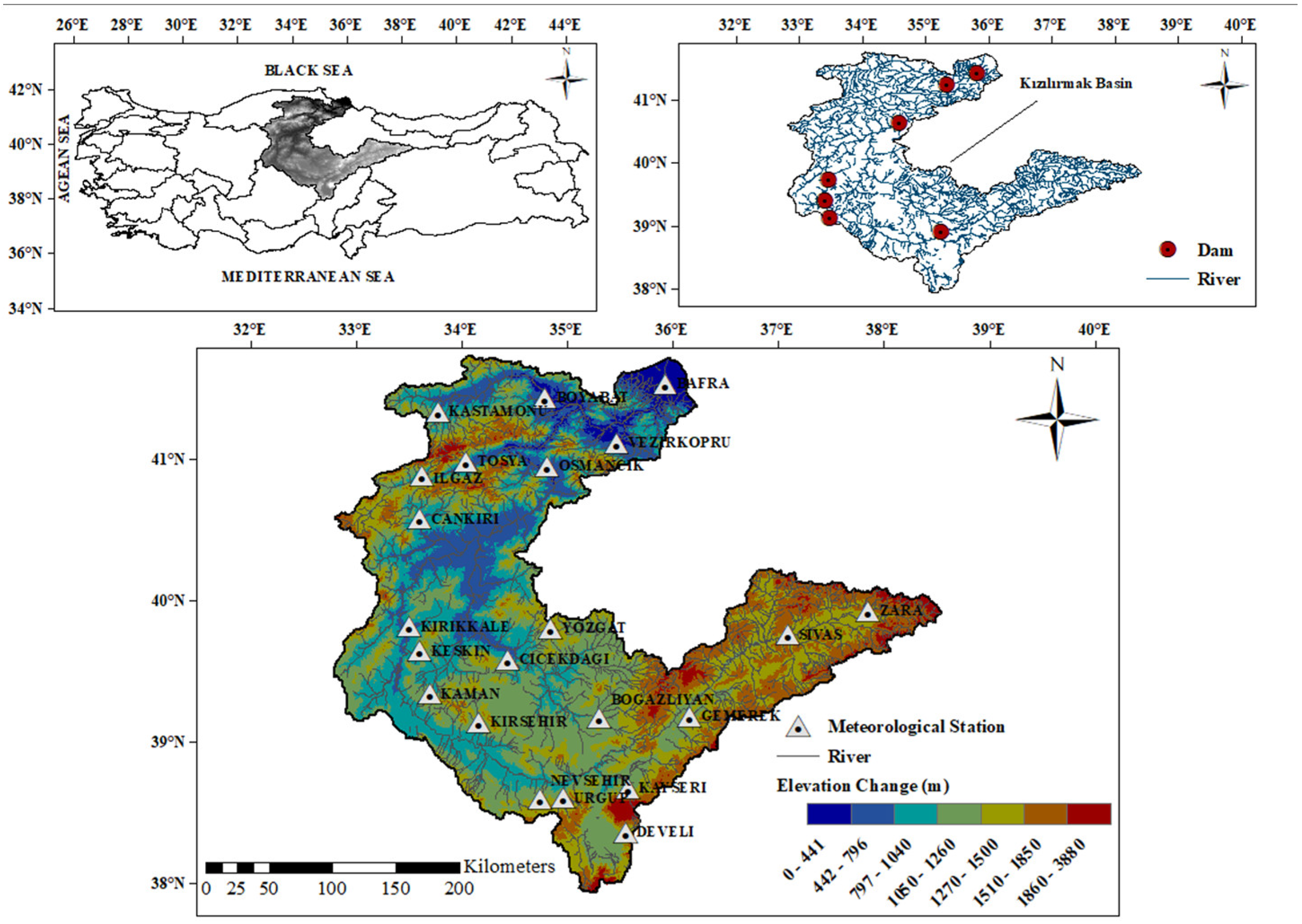
2.1. The Study Area

The study area is geographically located at 37°56′–41°44′ N latitudes and 32°48′–38°24′ E longitudes, with a land surface area of 82,082 km², which equates to about 10% of the surface area of Turkey (Figure 1). One of the nation’s primary water resources is the 1151 km long Kızılırmak River, which has an annual average flow rate of 184 m³/s at its Black Sea discharge. The Kızılırmak Basin showcases a diverse topography, featuring expansive plateaus, verdant meadows, and towering highlands. The basin’s altitude fluctuates between sea level and 3880 m above it, gradually decreasing from its upstream regions. The Kızılırmak Basin is an extensive area where we can see different topographical, geographical, and climatic features along the basin. The Upper Kızılırmak Region has a high and mountainous plateau feature and is the basin’s hilliest region. This region of the basin, which consists of high peaks, is bordered by mountainous areas from the north and south. Meadows and plateaus are mostly encountered in the Middle Kızılırmak Region of the basin. In this basin region, volcanic-origin mountains draw attention, and there are vast plains hills. The northern Anatolian and Kure Mountain ranges, located to the west of the Lower Kızılırmak Region, constitute the basin’s border with the Western Black Sea Basin. These mountain ranges act as a barrier against humid air masses from coastal regions, and because of this, they significantly affect the basin’s climate. A typical dry climate is dominant in a large part of the basin, and the Black Sea climate characteristics and effects are observed in the northern part of the basin. According to the results of previous analyses of the basin, agricultural lands, fertile forest lands, and degraded forest lands constitute the most significant land uses in the basin. Approximately 73% of the basin, 5,960,665 ha of the general area, consists of agricultural lands, and 7% comprises pasture areas used for livestock. The basin’s most widely produced agricultural products are cereals and legumes, such as sugar beet, potatoes, melons, and watermelons [75].

The mean temperature is around 10.5 °C, and the average annual precipitation is about 450 mm. The mean annual precipitation in the basin also varies yearly; while the minimum was 315 mm in 2013, the maximum was 606 mm in 2010. At the same time, differences in the precipitation data of the stations are observed because of the effect of the distance from the sea and the high elevation range in the basin. While the mean annual precipitation is 760 mm at Bafra meteorology station (103 m altitude), it decreases to 342 mm at Çiçekdağı meteorology station (900 m altitude). The spring months of April and May in the basin experience the most precipitation, while July and August in the summer experience the least. The monthly precipitation data between 1960 and 2020 were obtained from the General Directorate of Meteorology (MGM) of Turkey.

2.2. Precipitation Drought Indices

In this study, the SPI, ZSI, CZI, and MCZI methods were applied to the monthly total precipitation data observed from 1960 to 2020 at 22 stations in the Kızılırmak Basin. The results are classified in

Table 1. The classification of droughts for the SPI, ZSI, CZI, and MCZI [76].

SPI/ZSI/CZI/MCZI Values	Drought Category
≥2	Extreme Wet
1.5 to 1.99	Severe Wet
1.0 to 1.49	Moderate Wet
0.99 to −0.99	Near Normal
−1.0 to −1.49	Moderate Drought
−1.5 to −1.99	Severe Drought
≤−2.0	Extreme Drought

, and it was determined which intensity–time drought was observed at which observation station. The L-moments method was used to localize the results and obtain the rotation periods, and spatial visualization was carried out with the IDW method. The methods are listed in the following headings.

2.2.1. Standardized Precipitation Index (SPI)

The SPI is one of the most preferred drought indices and is well known, especially when studying meteorological droughts [77,78]. Historical long-term precipitation data are used to determine drought with the SPI method. This method determines the probability distribution function that best fits the observed rainfall data. The SPI values are computed following the computation of the cumulative probability values using the identified probability distribution function [79]. Since precipitation data can often fit the gamma distribution, the SPI values are calculated using a probability density function of the gamma distribution (Equation (1)) [80].

$$\mathrm{g}(\mathrm{x})={\displaystyle \frac{1}{{\mathrm{\beta }}^{\mathrm{\alpha }}\mathrm{T}(\mathrm{\alpha })}}{\mathrm{x}}^{(\mathrm{\alpha }-1)}{\mathrm{e}}^{{\displaystyle \frac{-\mathrm{x}}{\mathrm{\beta }}}}\hspace{0.33em}\hspace{1em}\hspace{0.33em}\hspace{0.33em}(\mathrm{x}>0)$$

(1)

In Equation (1), T (a) represents the α gamma function and x (mm) represents the precipitation amount (x > 0); α is a shape parameter (α > 0); and β is taken as the scale parameter (β > 0). The α and β parameters of the gamma distribution are calculated by the relations provided in Equations (2) to (4), depending on the number of sample data.

$$\mathrm{A}=\ln (\overline{\mathrm{x}})-{\displaystyle \frac{{\displaystyle \sum \ln (\mathrm{x})}}{\mathrm{n}}}$$

(2)

In Equation (2), $\overline{x}$ indicates the average of the precipitation data and n indicates the number of data.

$$\mathrm{\alpha }={\displaystyle \frac{1}{4\mathrm{A}}}\left(1+\sqrt{1+{\displaystyle \frac{4\mathrm{A}}{3}}}\right)$$

(3)

$$\mathrm{\beta }={\displaystyle \frac{\overline{\mathrm{x}}}{\mathrm{\alpha }}}$$

(4)

By finding the α and β parameters, the cumulative probability value of the precipitation value in any month is converted into the standard normal Z variable expressing the SPI values. Please review [81] for detailed information about the method. Accordingly, there are statistical data that we need when applying the SPI method. These are the arithmetic mean and standard deviation of the precipitation series observed during the study period. The SPI equation depending on these data is shown in Equation (5).

$$\mathrm{S}\mathrm{P}{\mathrm{I}}_{\mathrm{i}}={\displaystyle \frac{{\mathrm{P}}_{\mathrm{i}}-\overline{\mathrm{P}}}{{\mathrm{\sigma }}_{\mathrm{P}}}}$$

(5)

Here, ${\mathrm{P}}_{\mathrm{i}}$ represents the precipitation of any time, $\overline{\mathrm{P}}$ is the arithmetic average of the series and ${\mathrm{\sigma }}_{\mathrm{P}}$ represents the standard deviation of the series. The obtained drought data indicate the situation of the drought in that period according to the value ranges in Table 1.

2.2.2. Z-Score Index (ZSI)

The ZSI differs from the SPI as it does not require data adjustment to fit the gamma or Pearson type III distribution. The ZSI represents how many standard deviations a precipitation value is above or below the average [82]. The following equation can be used to compute the ZSI [80].

$$\mathrm{Z}\mathrm{S}\mathrm{I}={\displaystyle \frac{{\mathrm{P}}_{\mathrm{i}}-\overline{\mathrm{P}}}{\mathrm{S}\mathrm{D}}}$$

(6)

In this equation, the ZSI stands for the standardized variable precipitation score, $P_i$ is the average of precipitation, $\overline{\mathrm{P}}$ is the mean total precipitation, and SD is the standard deviation. The results are evaluated as in Table 1.

2.2.3. China-Z Index (CZI)

Since 1995, the Chinese National Climate Center has utilized variations of the CZI to monitor the drought conditions across the country [42,45,49]. The China-Z Index is related to the Wilson–Hilferty cube root transformation [83]. If precipitation follows the Pearson type III distribution, the CZI can be calculated using the following formula.

$$\mathrm{C}\mathrm{Z}{\mathrm{I}}_{\mathrm{i}\mathrm{j}}={\displaystyle \frac{6}{{\mathrm{C}}_{\mathrm{s}\mathrm{i}}}}\times {\left({\displaystyle \frac{{\mathrm{C}}_{\mathrm{s}\mathrm{i}}}{2}}\times {\mathrm{\varphi }}_{\mathrm{i}\mathrm{j}}+1\right)}^{1/3}-{\displaystyle \frac{6}{{\mathrm{C}}_{\mathrm{s}\mathrm{i}}}}+{\displaystyle \frac{{\mathrm{C}}_{\mathrm{s}\mathrm{i}}}{6}}$$

(7)

where i is the time scale of interest and j is the current month; CZI_ij means the CZI’s amount of the current month (j) for period i; C_si is the coefficient of skewness; and φ_ij is the standardized variation [80]. The CZI data found are evaluated and categorized according to Table 1.

2.2.4. Modified China-Z Index (MCZI)

The MCZI is calculated in the same way as the CZI, only the precipitation median is used instead of the average of precipitation data [84]. The values found after applying the MCZI method are classified according to the value ranges provided in Table 1 for the determining of drought.

2.3. Regional Frequency Analysis (RFA) and L-Moment Statistics

RFA aims to create a homogeneous region from the selected stations [85]. With regionalization, it is accepted that the frequency distribution in all the stations is the same. In the equation Qi (F) = μi q (F), F represents the probability of not being exceeded, μi represents the mean at station i, and q (F) represents the regional growth factor that is the same for each station. After obtaining the q (F) value due to RFA, the Qi (F) value of the hydrological variable at the station it belongs to can be obtained for the F recurrence by multiplying this value with the average of the desired station. In a region where there are N stations, the Qi (F) value of the hydrological variable at the station it belongs to can be obtained for the F recurrence by multiplying the average of the i station [86]. RFA consists of several stages listed in the following subheadings. Since the L-moments and L-moment ratios are used in all of these stages, this version of the indicator flood method is called the regional L-moment method [87].

2.3.1. L-Moments and L-Coefficients

Hosking developed the L-moments approach [59,88]. L-moments are commonly employed to solve parameter estimation, regionalization, and distribution identification issues. In this study, the probability-weighted moments method developed by Greenwood et al. [89] is used, and the following equation defines the linear functions of L-moments:

$$\mathrm{\beta }={\displaystyle \underset{0}{\overset{1}{\int }}\mathrm{x}(\mathrm{F})}{\mathrm{F}}^{\mathrm{j}}\mathrm{d}\mathrm{F}$$

(8)

Here, F = F(x), the cumulative distribution function (CDF) of the random variable x; x = x(F), the inverse of the CDF, defined as a variable function; and βj is the jth probability-weighted moment. As can be seen from Equation (8), when j = 0, the 0th probability-weighted moment is equal to the overall mean of the distribution. Linear moments are defined as linear combinations of moments defined using Equation (8) as follows.

$${\mathrm{\lambda }}_1={\mathrm{\beta }}_0$$

(9)

$${\mathrm{\lambda }}_2=2{\mathrm{\beta }}_1-{\mathrm{\beta }}_0$$

(10)

$${\mathrm{\lambda }}_3=6{\mathrm{\beta }}_2-6{\mathrm{\beta }}_1+{\mathrm{\beta }}_0$$

(11)

$${\mathrm{\lambda }}_4=20{\mathrm{\beta }}_3-30{\mathrm{\beta }}_2+12{\mathrm{\beta }}_1-{\mathrm{\beta }}_0$$

(12)

Here, λj is the jth L-moment of the distribution. By proportioning the L-moments, the L-coefficients of the distribution are defined as follows.

$$\mathrm{\tau }\equiv \mathrm{L}-\mathrm{C}\mathrm{o}\mathrm{e}\mathrm{f}\mathrm{f}\mathrm{i}\mathrm{c}\mathrm{i}\mathrm{e}\mathrm{n}\mathrm{t} \mathrm{o}\mathrm{f} \mathrm{v}\mathrm{a}\mathrm{r}\mathrm{i}\mathrm{a}\mathrm{t}\mathrm{i}\mathrm{o}\mathrm{n}={\displaystyle \raisebox{1ex}{${\mathrm{\lambda }}_2$}\!\left/ \!\raisebox{-1ex}{${\mathrm{\lambda }}_1$}\right.}$$

(13)

$${\mathrm{\tau }}_3\equiv \mathrm{L}-\mathrm{S}\mathrm{k}\mathrm{e}\mathrm{w}\mathrm{n}\mathrm{e}\mathrm{s}\mathrm{s} \mathrm{c}\mathrm{o}\mathrm{e}\mathrm{f}\mathrm{f}\mathrm{i}\mathrm{c}\mathrm{i}\mathrm{e}\mathrm{n}\mathrm{t}={\displaystyle \raisebox{1ex}{${\mathrm{\lambda }}_3$}\!\left/ \!\raisebox{-1ex}{${\mathrm{\lambda }}_2$}\right.}$$

(14)

$${\mathrm{\tau }}_4\equiv \mathrm{L}-\mathrm{K}\mathrm{u}\mathrm{r}\mathrm{t}\mathrm{o}\mathrm{s}\mathrm{i}\mathrm{s} \mathrm{c}\mathrm{o}\mathrm{e}\mathrm{f}\mathrm{f}\mathrm{i}\mathrm{c}\mathrm{i}\mathrm{e}\mathrm{n}\mathrm{t}={\displaystyle \raisebox{1ex}{${\mathrm{\lambda }}_4$}\!\left/ \!\raisebox{-1ex}{${\mathrm{\lambda }}_2$}\right.}$$

(15)

It is explained by Hosking and Wallis [60] that the L–coefficient of variation τ functions as the conventional coefficient of variation (standard deviation/µ); in other words, it quantitatively reflects the narrowness or breadth of the probability density function. The basis of the regionalization study performed by the L-moments method is based on the L-moments ratios calculated from the observed series at each station. Among the sample probability distributions, with the Z^DIST fitness test, the one that is closest to the theoretical relation between the L-kurtosis and L-skewness coefficients is chosen as the most suitable distribution for the region. Any mean recurring value at any point in the homogeneous region is obtained by multiplying the value provided by the standardized frequency curve. This curve is defined with the mean value estimated at that point. The following equation calculates the minimum drought index with the regionalized drought frequency analysis recurrence period.

$${\mathrm{I}}_{\mathrm{T}}=\mathrm{x}(\mathrm{F})\mathsf{\mu }$$

(16)

In this equation, I_T is the drought index value with a recurrence period of T years at that geographic point; F is the probability of the T-year mean recurrent drought index small stay (not exceeded) associated with the mean recurrence period by the expression F = 1 − 1/T, x(F), the inverse (variable function) of the cumulative function of the probability distribution found suitable for the standard drought index value whose average is equal to one (μ = 1); and μ is the average of the minimum drought indexes at that geographic point [87,90,91].

2.3.2. Non-Compliance Criterion According to L-Moments Method

The discordancy criterion is used to identify stations that may be too far from the mean of the congruent stations in the homogeneous assumed region. A non-conforming station is excluded from the regionalization analyses based on the L-moments in the homogeneous region. The following formula expresses the discordancy criterion [90,92].

$${\mathrm{D}}_{\mathrm{i}}={\displaystyle \frac{1}{3}}\mathrm{N}{({\mathrm{u}}_{\mathrm{i}}-\overline{\mathrm{u}})}^{\mathrm{T}}{\mathrm{A}}_{\mathrm{H}}^{-1}({\mathrm{u}}_{\mathrm{i}}-\overline{\mathrm{u}})$$

(17)

Here, the matrix form of the coefficients u_i, L-variation, L-kurtosis, L-skewness; T_i is the transpose of the matrix; $\overline{\mathsf{\mu }}$ is the unweighted group mean; A_H is the matrix and cross product of the sum of its squares and D_i is the discordancy measure for station i. D_i is defined by the number of stations in the area. If the calculated D_i value is greater than the critical D_i value, that station is indicated to be irregular [93]. The number of stations’ critical values are shown in

Table 2. Critical values for the discordancy measure.

Number of Stations	Critical Value	Number of Stations	Critical Value
5	1.333	11	2.632
6	1.648	12	2.757
7	1.917	13	2.869
8	2.140	14	2.971
9	2.329	≥15	3
10	2.491

.

2.3.3. Homogenization Test

The region’s homogeneity is assessed using homogeneity measurements to determine whether the selected region is homogeneous after the discordancy test. Homogeneity metrics are based on simulating 500 homogenous regions with population parameters equal to the regional average sample l-moment ratios [93]. The L-moments-based homogeneity test H_k statistics are provided by Equation (18).

$${\mathrm{H}}_{\mathrm{K}}={\displaystyle \frac{({\mathrm{V}}_{\mathrm{K}}-{\mathrm{\mu }}_{\mathrm{v}})}{{\mathrm{\tau }}_{\mathrm{v}}}}$$

(18)

In this equation, three different H_k are defined with k = 1, 2, 3, of which H₁ is more determinant, as it depends on Hosking [59], experiences and on the L-variation coefficient. Therefore, H₁ becomes more important. Here, V_k is the weighted standard deviation of the kth L-coefficient, while μ_v and σ_v are the mean and standard deviation of the V_k values obtained from 500 synthetic series. If the value of the homogeneity statistic is less than 1 (H_k < 1), the region is considered to be strictly homogeneous, probably heterogeneous when 1 ≤ H ≤ 2, and certainly heterogeneous when H ≥ 2 [87].

2.3.4. Choosing ZDIST Goodness-of-Fit Tests

The best fit in the RFA indicates a single probability distribution for data obtained from stations in the selected homogenous region. The goodness-of-fit test is used to select the most appropriate regional frequency distribution (Z^DIST) [93,94]. Equations (19)–(21) are used to compute the Z^DIST statistics by comparing the following equations.

$${\mathrm{\beta }}_4={\mathrm{N}}_{\mathrm{S}\mathrm{I}\mathrm{M}}^{-1}.{\displaystyle \sum _{\mathrm{m}=1}^{{\mathrm{N}}_{\mathrm{S}\mathrm{I}\mathrm{M}}}{\mathrm{\tau }}_4^{\mathrm{m}}-}{\mathrm{\tau }}_4^{\mathrm{R}}$$

(19)

$${\mathrm{\sigma }}_4={\left.\left\{{({\mathrm{N}}_{\mathrm{S}\mathrm{I}\mathrm{M}}-1)}^{-1}.\right.\left[{\displaystyle \sum _{\mathrm{m}=1}^{{\mathrm{N}}_{\mathrm{S}\mathrm{I}\mathrm{M}}}({\mathrm{\tau }}_4^{\mathrm{m}}-}{\mathrm{\tau }}_4^{\mathrm{R}}{)}^2-{\mathrm{N}}_{\mathrm{S}\mathrm{I}\mathrm{M}}.{\mathrm{\beta }}_4^2\right]\right\}}^{0.5}$$

(20)

$${\mathrm{Z}}^{\mathrm{D}\mathrm{I}\mathrm{S}\mathrm{T}}={\displaystyle \frac{\left({\mathrm{\tau }}_4^{\mathrm{D}\mathrm{I}\mathrm{S}\mathrm{T}}-{\mathrm{\tau }}_4^{\mathrm{R}}+{\mathrm{\beta }}_4\right)}{{\mathrm{\sigma }}_4}}$$

(21)

In these equations, ${\mathsf{\tau }}_4^R$ and ${\mathsf{\tau }}_4^m$ are the regional L-Basque coefficients determined from the recorded series and the m simulation; β₄ is the correction term for the bias in the estimation of the regional mean L-squared coefficient determined from the recorded series; σ4 is the standard deviation of the regional mean L-Basque coefficient determined from the recorded series; and ${\mathsf{\tau }}_4^{DIST}$ is the theoretical L-squared coefficient of the candidate probability distribution. Nsim denotes the number of simulations (synthetic series) carried out by the Kappa distribution [94]. The N_sim 500 is used in this study, which is recommended by Hosking and Wallis (1997) [62]. The software (Version 3.04) presented by Hosking was employed and Z^DIST statistics values of the generalized logistic (GLO), Pearson type III (PE3), generalized extreme value (GEV), generalized normal (GNO) and generalized Pareto (GPA) distributions were determined [95,96].

2.3.5. Inverse Distance-Weighted Interpolation Method (IDW)

The IDW method is one of the most popular non-geostatistical methods in the literature [97]. This method uses interpolation to compute the cell values of unknown points based on the values of known sample points. It uses local interpolation since it only creates estimates from surrounding spots. The method is based on the notion that local points have a higher weight on the interpolated surface than remote points [98,99]. A mathematical expression called Shepard’s method is used in IDW interpolation [100]. The general equations for the method are given below.

$$\mathrm{F}\left(\mathrm{x},\mathrm{y}\right)=\sum _{\mathrm{i}=1}^{\mathrm{n}}{\mathrm{w}}_{\mathrm{i}}\ast {\mathrm{f}}_{\mathrm{i}}$$

(22)

$${\mathrm{w}}_{\mathrm{i}}={\mathrm{h}}_{\mathrm{i}}^{-\mathrm{p}}/\sum _{\mathrm{i}=1}^{\mathrm{n}}{\mathrm{h}}_{\mathrm{i}}^{-\mathrm{p}}$$

(23)

In the equations, p refers to the exponent known as the force parameter, h_i is the spatial distance between the sample points and the interpolated points, w_i is the sum of the weight values, which should be 1, and f_i refers to the known height values. This IDW method has been applied in ArcGIS 10.8 software, Geographical Information Systems software, and the maps prepared are included in the application section. The specific purpose of using the IDW interpolation technique in the study is to achieve a better and more practical performance in predicting precipitation in the study area compared to methods such as Kriging and spline, as reported in the literature [101,102]. The IDW method has been employed to obtain more accurate predictions in intermediate regions based on the characteristics of the dataset and the analysis requirements [103]. Unlike the Kriging method, the IDW method is not a complex and time-consuming method because it does not require estimating the variogram model [104]. Due to these advantages of the IDW method, it has been widely used in recent years [105,106,107,108,109,110]. The relationship between the materials and methods used in this study and the workflow chart of the study are set out below (Figure 2).

3. Results

Before the drought analysis and regionalization study with the L-moments method, the descriptive statistics of the data were examined, and the results are summarized with the location information and Köppen climate type [111] in

Table 3. Statistical parameters of the Kızılırmak Basin data.

Station Name (Altitude, m)	Period	Latitude (°N)	Longitude (°E)	Köppen Climate Type *	Range	Mean	SD	Kurtosis	Skewness	Coefficient of Variation
					(0-mm)	(mm)	(mm)	(mm)	(mm)	(%)
Bafra (103)	1960–2020	41.55	35.92	Csa	343.90	63.29	44.98	3.33	1.40	71.07
Boğazlıyan (1070)	1960–2020	39.19	35.25	Csb	159.90	30.29	25.46	1.61	1.12	84.03
Boyabat (350)	1960–2020	41.46	34.79	Cfb	241.50	34.48	28.44	6.47	1.91	82.48
Çankırı (755)	1960–2020	40.61	33.61	Cfa	149.80	34.63	27.48	1.31	1.13	79.34
Çiçekdağı (900)	1972–2020	39.61	34.42	BSk	171.10	28.51	23.79	2.46	1.19	83.47
Develi (1204)	1960–2020	38.37	35.47	Csa	159.60	30.23	26.28	1.10	1.02	86.95
Gemerek (1182)	1960–2020	39.19	36.08	Csb	160.00	32.98	27.06	1.50	1.07	82.04
Ilgaz (885)	1960–2020	40.92	33.63	Cfb	216.60	40.00	31.22	3.06	1.34	78.06
Kaman (1075)	1960–2020	39.37	33.71	Csb	246.20	38.51	33.43	2.80	1.25	86.80
Kastamonu (800)	1960–2020	41.37	33.78	Cfb	278.70	41.77	32.57	5.62	1.80	77.99
Kayseri (1094)	1960–2020	38.69	35.50	Csa	164.70	32.45	25.82	0.93	0.92	79.58
Keskin (1140)	1960–2020	39.67	33.61	Csb	145.90	33.68	27.49	0.80	1.02	81.61
Kırıkkale (751)	1960–2020	39.84	33.52	BSk	172.70	31.95	27.37	1.68	1.16	85.65
Kırşehir (1007)	1960–2020	39.16	34.16	Csa	161.40	31.94	26.83	1.18	1.03	84.01
Nevşehir (1260)	1960–2020	38.62	34.70	Csb	148.80	34.54	27.73	0.43	0.82	80.28
Osmancık (419)	1976–2020	40.98	34.80	BSk	139.00	33.04	25.00	0.78	0.98	75.65
Sivas (1294)	1960–2020	39.74	37.00	Dsb	154.80	36.49	28.15	0.61	0.84	77.13
Tosya (870)	1960–2020	41.01	34.04	Cfb	157.20	39.17	28.40	1.04	0.99	72.49
Ürgüp (1068)	1964–2020	38.62	34.91	Csb	138.30	30.19	25.26	1.01	0.99	83.68
Vezirköprü (378)	1960–2020	41.14	35.45	Cfb	172.00	47.81	30.03	0.73	0.77	62.81
Yozgat (1301)	1960–2020	39.82	34.82	Csb	192.30	48.74	38.64	0.44	0.86	79.27
Zara (1338)	1960–2020	39.89	37.75	Dsb	171.40	43.35	33.65	0.63	0.90	77.64

Notes: * Csa: climate with mild winters and very hot and dry summers; Csb: climate with mild winters, warm summers and dry climate; Cfb: climate with warm winters and summers, rainy in all seasons; Cfa: severe winter, rainy in all seasons, hot in summer; BSk: semi-arid steppe climate (cold) Dsb: winter is severe, summer is dry and cool.

. As Table 3 shows, the kurtosis coefficient for all the stations is greater than zero, indicating a platykurtic characteristic, which means the distributions are flatter compared to a normal distribution. The Nevşehir (1260) and Yozgat (1301) stations have the lowest kurtosis coefficients, indicating that their data distributions are flatter and contain fewer outliers. In contrast, the Boyabat (350) and Kastamonu (800) stations have the highest kurtosis values, suggesting that their data distributions are more peaked and contain more outliers. In evaluating the skewness coefficient results, the skewness coefficients of all the stations provide close results. In addition, the skewness coefficients of all the stations are greater than zero, indicating a right-skewed distribution. This means that the data distributions are asymmetrical, with a longer tail on the right side. The coefficient of variation refers to the data distribution around the arithmetic mean. Table 3 shows that the coefficient of variation of the data of the Kızılırmak Basin stations varies between 62.81% and 86.95%. Since the Develi (1204) station has the highest coefficient of variation, its probability density function indicates the greatest variability among the stations. Conversely, the Vezirköprü (378) station, with the lowest coefficient of variation, shows values that are more homogeneously distributed around the arithmetic mean. According to the descriptive statistics of the stations, it seems that the stations in the Kızılırmak Basin are compatible. Aktürk et al. [112] determined the most appropriate probability distribution for the selected meteorological stations in the Kızılırmak Basin at the 0.1, 0.05 and 0.01 significance levels according to the Kolmogorov–Smirnov and χ2 (chi-square) statistics. Here, they found that the Pearson type III probability distribution is the most suitable distribution for monthly total precipitation data.

3.1. Drought Indices Results

The droughts examined on a 12-month time scale for each station and drought class, the average drought severity and average drought duration, the longest duration of the examined droughts as well as their start–end times, the maximum drought severity (

Table 4. Maximum drought severity at each station in the Kızılırmak Basin according to the SPI, MCZI, CZI and SPI results at a 12-month time scale.

Station Name	Maximum Drought Severity (for SPI)		Maximum Drought Severity (for MCZI)		Maximum Drought Severity (for CZI)		Maximum Drought Severity (for ZSI)
	Severity	Time	Severity	Time	Severity	Time	Severity	Time
		(Year/Month)		(Year/Month)		(Year/Month)		(Year/Month)
Bafra	−3.46	2014/8	−3.49	2014/5	−2.83	2014/3	−2.83	2014/8
Boğazlıyan	−3.37	2017/5	−3.72	2017/6	−3.7	2017/5	−2.58	2017/5
Boyabat	−2.67	2017/9	−6.87	2017/9	−7.92	2017/9	−2.03	2017/9
Çankırı	−3.07	2007/10	−6.5	1986/8	−2.75	1986/8	−2.5	2007/10
Çiçekdağı	−2.6	2014/1	−3.23	2012/7	−2.46	2014/2	−2.22	2014/1
Develi	−4.41	2014/4	−2.86	2014/5	−2.91	2014/5	−3.36	2014/4
Gemerek	−2.47	2001/10	−4.44	2001/10	−3.52	2001/10	−2.17	1995/3
Ilgaz	−2.22	1962/7	−4.73	1962/7	−5.69	1962/8	−1.68	1962/7
Kaman	−2.69	2020/12	−5.98	2005/1	−2.92	2005/1	−2.3	2020/12
Kastamonu	−2.4	1994/9	−5.8	1994/8	−2.49	1964/5	−2.07	1994/9
Kayseri	−2.87	2016/11	−7.2	2016/6	−3.15	2016/6	−2.36	2016/11
Keskin	−2.93	2017/5	−8.55	2017/3	−3.14	2017/3	−2.46	2017/9
Kırıkkale	−3.02	2007/10	−2.8	2008/6	−2.43	2007/10	−2.52	2007/10
Kırşehir	−2.51	1974/8	−2.59	1995/2	−2.33	1995/2	−2.19	1974/8
Osmancık	−2.7	2014/2	−3.88	2014/3	−2.74	2014/3	−2.23	2014/2
Sivas	−2.76	1973/10	−2.84	2014/5	−2.38	2014/5	−2.42	1973/10
Tosya	−2.83	2020/12	−2.57	2020/12	−2.7	2020/12	−2.41	2020/12
Ürgüp	−3.33	2012/9	−2.95	2014/5	−2.88	2014/5	−2.71	2012/9
Vezirköprü	−3.89	2014/4	−2.83	2014/5	−2.7	2014/4	−3.18	2014/4
Yozgat	−3.24	2001/10	−2.87	1974/6	−2.47	1974/6	−2.79	2001/10
Zara	−3.68	2014/5	−4.17	2012/11	−3.23	2012/11	−3.02	2014/5

), and the years when extreme droughts occurred are detailed in Appendix B. According to the SPI, ZSI, and CZI results, the total drought events were mainly experienced at the Kırşehir (1007) station, and according to the MCZI results, at the Sivas (1294) station. When the average drought duration is examined, it is observed that the average duration ranged between 5.11 and 2.93 for the SPI results, 5.5 and 2.88 for the ZSI results, and 5.5 and 2.90 for the CZI results. The maximum average drought duration for the three indices was obtained at the Zara (1338) station, and the minimum was obtained at the Keskin (1140) station. However, according to the MCZI results, the average drought duration varies between 4.91 and 2.52. The maximum average drought duration was obtained at the Boğazlıyan (1070) and Boyabat (350) stations, and the minimum was obtained at the Keskin (1140) station. However, according to the MCZI results, the average drought duration varied between 4.91 and 2.52. The maximum value was obtained at the Boğazlıyan (1070) and Boyabat (350) stations, and the minimum value was obtained at the Keskin (1140) station. In the study area, the longest experienced drought period was 31 months, from April 2012 to October 2014 at the Ürgüp (1068) station, and the index results for each station showed approximate values. At the same time, when the average drought severity is evaluated, the index results for each station show close values. For example, the average drought severity for the Tosya (870) station in the north of the basin was found to be −1.52 according to the SPI values and −1.49 for the MCZI. For the Zara (1338) station located in the east of the basin, it was found to be −1.60 according to the ZSI values and −1.59 for the CZI. The results showed slight differences in the maximum drought severity for each index, but extremely severe drought events were experienced at all the stations in the basin. In particular, for many stations, the maximum drought severity obtained by the MCZI method was higher than the values calculated by the other methods. Thus, for the Kaman (1075) station, the maximum severity was found to be −2.69 (December 2020) with the SPI method, −2.30 (December 2020) with the ZSI method, −2.92 (January 2005) with the CZI method, and −5.98 (March 2014) with the MCZI method. When years with extremely severe drought events (major drought events) and when long-term drought events are evaluated together, the four different indices’ results revealed that these droughts mainly occurred in the 2000s. The selected study area is also affected by the most severe and widespread drought events in Turkey [19,113,114,115]. One of the most important results of the drought analysis in this study is that the MCZI method is not suitable to be used in some stations (Keskin (1140), Kayseri (1094), Boyabat (350), Çankırı (755), Kaman (1075), Kastamonu (800), Ilgaz (885), Gemerek (1182), Zara (1338)) because it provides extraordinary results compared to other index results. In addition to the high results obtained with the MCZI method at the Ilgaz (885) and Boyabat (350) stations, the CZI results for only these two stations among all the stations studied in the basin also differed from the other index results. Therefore, besides the MCZI method, the CZI method is unsuitable for use at the Boyabat (350) and Ilgaz (885) stations.

One of the notable findings of this study is the observed increase in the drought severity values for the Zara station (1338), located in the Upper Kızılırmak basin, starting from the 2000s. Additionally, extreme drought occurrences were found to only occur during this period. The annual average precipitation in the Upper Kızılırmak Basin varies depending on the elevation and the influence of moisture-laden air masses within the basin. The region has a parallel increase with the elevation, with the annual average precipitation being 396 mm in Gemerek at an elevation of 1182 m, 438 mm in Sivas at 1294 m, and 520 mm in Zara at 1338 m. The relatively high precipitation at the Zara station is attributed to the tendency of air masses originating from the Black Sea to traverse the mountainous terrain to the north of the basin and reach the basin [116]. However, in Zara, which has a semi-arid climate condition, decreasing trends in the annual and spring precipitation and increasing temperatures have been observed starting from the 2000s [117]. Therefore, this situation has led to more severe and effective fluctuations in the precipitation and temperature in the region due to global climate change, resulting in severe and extreme drought conditions.

3.2. Regionalization with L-Moments Method

3.2.1. Calculation of L-Coefficients, Non-Compliance Criterion and Homogeneity

Monthly precipitation data from 22 meteorological stations in the Kızılırmak Basin up to 2020 were used to calculate the annual maximum drought severity values for four drought indices at a 12-month time scale. The basis of the regionalization study performed by the L-moments method is based on the L-moments ratios calculated from the observed series at all the stations in the region. For this reason, at the beginning of the study, the L-moments ratios, which are defined as the L-variation, L-skewness, and L-kurtosis coefficients of the SPI, MCZI, CZI, and ZSI values of the 22 meteorology stations, were calculated. A discordancy test was carried out using these ratios for the regionalization study. So, firstly, the discordancy test was performed for each of the SPI, MCZI, CZI and ZSI values of the 22 meteorology stations and the results of the discordancy test are shown in

Table 5. Summary of discordancy and homogeneity test results for the SPI, MCZI, CZI, and ZSI indices.

Indices	Discordant Stations	D Statistics	H1	H2	H3
SPI	17648 Ilgaz	3.27	−1.35	−1.50	−0.96
MCZI	17648 Ilgaz	3.90	0.02	0.87	3.38 *
CZI	17648 Ilgaz, 17620 Boyabat	4.73, 5.10	−1.25	−1.68	−1.57
ZSI	17648 Ilgaz, 1122 Vezirköprü	3.49, 3.19	−2.24	−2.01	−0.75

Notes: * Not homogeneous.

. As can be seen in Table 5, only the Ilgaz (885) station for the SPI and MCZI, Ilgaz (885) and Boyabat (350) stations for the CZI, and Ilgaz (885) and Vezirköprü (378) stations for the ZSI were determined to be discordant and removed from the study area. The Ilgaz (885) station was found to be discordant in all four of the SPI, MCZI, CZI, and ZSI drought indices.

Secondly, in the regionalization study, the homogeneity test was performed for each of the SPI, MCZI, CZI, and ZSI; the homogeneity test results are shown in Table 5. As can be seen in Table 5, it has been determined that the Kızılırmak Basin is a single homogeneous region because the H1 and H2 values found for the SPI, MCZI, CZI, and ZSI values are less than one. Except for the MCZI, the H3 value of the other three indices is less than one, and according to the H3 value, it has been determined that the Kızılırmak Basin is a single homogeneous region.

3.2.2. Choosing ZDIST Goodness-of-Fit Tests

After the discordance and homogeneity test stages, graphical methods were applied to determine the most appropriate probability distribution [118,119,120]. Graphical methods visually determine the proper distribution by using the points of the “L-skewness (t3)↔L-Kurtosis (t₄^R)” coefficients of each station and the mean point of these point values. In addition, Figure 3 is drawn to visually show the appropriate distribution of the SPI, MCZI, CZI, and ZSI. In Figure 3, for the SPI, MCZI, CZI, and ZSI values, the “t₄↔t₃” points calculated from the data of the stations with the “τ₄↔τ₃” curves of each station and the mean point of these point values are provided. As can be seen from these figures, it is interpreted that if the mean of the t₄↔t₃ points of the series (each station) is closer to the τ₄↔τ₃ curve of the distribution, that distribution is the most appropriate distribution. This way, it is determined visually that the most appropriate distribution for the MCZI values is the GLO distribution. However, it is determined that the appropriate distribution for the SPI and ZSI values is the PE3 and GNO distributions. The appropriate distribution for the CZI values is PE3, GNO, and GEV distributions, and it is impossible to determine the most suitable distribution visually.

The regional L-variation (t₂^R), L-skewness (t₃^R), and L-kurtosis (t₄^R) coefficients were calculated by averaging the point coefficients with the weight coefficients obtained by dividing the length of the single series by the total series length. Based on the fact that there is a general main distribution and that the three-parameter potential distributions are its special forms, synthetic series were derived with the four-parameter Kappa distribution, whose parameter values were determined using the regional L-coefficients [87,121]. After 500 synthetic series simulations were performed, the Z^DIST statistics were calculated for all the candidate distributions. In

Table 6. Goodness-of-fit measures for the SPI, MCZI, CZI, and ZSI indices.

Indices	GLO	GEV	GNO	PE3	GPA
SPI	5.64	−1.07	0.52	0.45 *	−13.35
MCZI	1.63 *	−3.23	−2.650	−3.00	−12.77
CZI	6.00	−0.77 *	1.05	1.01	−12.87
ZSI	5.15	−1.63	0.51	0.38 *	−13.31

Notes: * absolute Z-statistic value that is less than 1.64 and closest to zero.

, the Z^DIST statistics values for the GLO, GEV, GNO, PE3 and GPA distributions are available.

Hosking and Wallis [87] and Peel et al. [118] point out that visual inspection of the L-moment ratio diagram should not be the only criterion when choosing the optimal distribution. For this reason, they argue that acceptable distributions should include a measure of goodness-of-fit testing to define them. For a probability distribution to represent a homogeneous region, its Z^DIST statistic must be in the range −1.64 < Z^DIST < +1.64. Among the distributions satisfying this condition, the one with the smallest absolute value of Z^DIST statistics is the most appropriate. Therefore, distributions with the smallest absolute value for Z^DIST statistics were chosen at the beginning. As seen in Table 6, the Z^DIST statistic for the MCZI is the most appropriate distribution, with the smallest value of 1.63 compared to the others. Since the Z^DIST statistics are smaller than for the other distributions, the PE3 distribution is the most appropriate for the SPI and ZSI. In contrast, the GEV distribution is the most appropriate for the CZI index.

Table 7. Regional parameters of all the distributions for the SPI, MCZI, CZI, and ZSI indices.

Indices	GLO			GEV			GNO			PE3			GPA
	Location	Scale	Shape	Location	Scale	Shape	Location	Scale	Shape	Location	Scale	Shape	Location	Scale	Shape
SPI	0.98	0.625	−0.019	0.594	1.084	0.249	0.978	1.108	−0.04	1	1.109	0.119	0.978	1.108	−0.04
MCZI	0.907	0.674	−0.084	0.421	0.96	−0.026	0.897	1.193	−0.171	1	1.218	−0.512	0.897	1.193	−0.171
CZI	1.003	0.608	0.003	0.625	1.077	0.29	1.004	1.078	0.007	1	1.078	−0.02	1.004	1.078	0.007
ZSI	1.038	0.562	0.041	0.685	1.033	0.359	1.042	0.997	0.084	1	1.002	−0.253	1.042	0.997	0.084

presents the regional parameters of all the distributions of the SPI, MCZI, CZI, and ZSI values calculated using the regional L-coefficients.

Table 8. Regional standard quantile of the severity of the SPI, MCZI, CZI, and ZSI drought indices in Kızılırmak Basin.

Indices	Return Periods (Years)	5	10	25	50	100	200	500	1000
SPI	PE3	1.926	2.434	2.986	3.348	3.676	3.98	4.352	4.616
MCZI	GLO	1.897	2.532	3.36	4.006	4.682	5.393	6.396	7.205
CZI	GEV	1.935	2.406	2.871	3.142	3.362	3.541	3.729	3.84
ZSI	PE3	1.853	2.254	2.664	2.919	3.143	3.343	3.578	3.739

presents the standard quantile estimates for a single homogeneous region. The standard quantile estimates for the four drought indices have very high values. The standard quantile estimates initially yielded similar results for the four drought indices. However, with the increase in the return period, it was observed that the standard quantile values of the MCZI increased more rapidly than the standard quantile values of the SPI, CZI, and ZSI. The rapid increase in the standard quantile values of the MCZI is because the MCZI provides higher results than the other indices at many stations in the basin. In addition, as can be seen in Table 8, extreme drought values were observed in all the indices after ten years.

The standard quantile function x(F) obtained from the appropriate distribution and the “flood index”, which is the mean of the annual series of flood peaks at “μ” at the relevant geographical point, were used to calculate the flood peak size with an average T-year recurrence period at any location [121]. This study calculated the standard quantile function for each index, as shown in Table 8. At the same time, many data, such as the latitude, longitude, and maximum temperature, were used to represent the average values of the drought severity for each drought index. However, no function that could represent the average of the drought severity values of the four drought indices could be obtained. For this reason, maps were obtained by using the IDW method to determine the probability of drought severity at any point in the basin where there are insufficient data [61,67,70]. The data to be used in the formation of probability maps of the drought severity values were calculated for each station by multiplying the average of the drought values of each station with the standard quantile function values one by one. Figure 4, Figure 5, Figure 6 and Figure 7 show the maps obtained by the IDW method using these drought severity values. In addition, the IDW method is arranged according to the one/standard deviation legend range in order to follow the intermediate values and highlight the peak values on the maps.

The primary purpose of the maps in Figure 4, Figure 5, Figure 6 and Figure 7 was to determine the future drought situation of any point. Thus, the legend values were taken differently from the classical value range of drought when drawing the maps. In this way, the maps in the figures can examine the changing effects of drought from north to south and east to west. The drought maps were created using the IDW method in ArcGIS 10.8, and the drought severity values for each pixel were obtained. Figure 4, Figure 5, Figure 6 and Figure 7 show the spatial distribution of the drought severity values for the eight fixed return periods (5, 10, 25, 50, 100, 200, 500, and 1000 years) that were obtained from the SPI-12, ZSI-12, CZI-12, and MCZI-12 analysis results in this study for the entire basin. In Figure 4, the drought increases further in the transition from east to west. While less drought is observed in the northern and southern ends, it is observed that there is more drought in the inner parts. It is thought that the reason for the low drought in the northern parts is the rainfall in the Black Sea, and the reason for the low drought in the southern parts is the rains that occur right behind the Taurus Mountains. Additionally, in the SPI index, more drought is observed in the Yozgat (1301) and Sivas (1294) stations and their surroundings. Figure 5 shows maps similar to the SPI index for the ZSI index. It is seen that drought increases as we move from north to south. As in the SPI index, it is seen that the drought increases further from east to west in the ZSI index. Figure 6 shows that the CZI and ZSI indices provide opposite results. Unlike the ZSI index, in the CZI index, a lot of drought is observed in the Boyabat (1070) and Ilgaz (885) stations, while less drought is observed in the Sivas (1294) station. This is because the observed precipitation data for the Boyabat (1070) and Ilgaz (885) stations are more skewed than those for the Sivas (1294) station. Figure 7 shows that while the Kayseri (1094) and Sivas (1294) stations are the driest regions in the MCZI index, the Vezirköprü (378), Osmancık (419) and Zara (1338) stations have less drought around them. In the SPI, ZSI and MCZI indices, the surroundings of the Sivas (1294) station appear to be drier. The Zara (1338) station and its surroundings appear less arid in the SPI, CZI and MCZI indices.

The percentages of the areal extent of the drought severity values for this return periods were shown in Figure 8. In Figure 8, fixed intervals are arranged for readers to understand the region’s drought severity values better. The maps and the graphs of the four drought indices show that as expected, the amount of drought severity increases with the increasing return period. In natural events (drought, flood, earthquake, etc.), the severity increases as the recurrence time increases [122].

3.3. Inverse Distance Weighted Interpolation Method (IDW)

In the 5-year return period, the SPI results show 18% of the basin has moderate drought and 82% severe drought; the ZSI results show 59% moderate drought and 41% severe drought; the CZI results indicate 9% moderate drought, 87% severe drought, and 3% extreme drought at the Ilgaz (885) and Boyabat (350) stations in the north; and the MCZI results show 15% moderate drought and 95% severe drought. For the 50-year return period, the SPI shows extreme droughts across the entire basin, and the ZSI shows 98% extreme droughts. During the 25-year return period, the CZI and MCZI results indicate that extreme droughts dominate the entire basin. To make this study applicable, regression analysis was performed using the longitude, latitude, altitude and frequency values as independent variables. The t values of the latitude, longitude, and frequency turned out to be greater than the critical t (t_crit) and the altitude was discarded simply because its t value was smaller than t_crit. In this study, linear regression equations in which the latitude, longitude, and frequency values were obtained using IDW maps of each drought index. The regression equations developed for each drought index are shown in

Table 9. Summary of the validation regression for means of the SPI, MCZI, CZI and ZSI indices developed using the IDW map data for each frequency (mean drought severity = a × (Lo) + b × (La) + c × (q).

Indices	Regression Coefficients		t Value of Coefficient
SPI	a	−0.0388	−75.46
	b	−0.0477	−105.98
	c	9.7022	−801.86
MCZI	a	−0.0867	−73.59
	b	−0.0373	−36.21
	c	17.7712	−641.75
CZI	a	0.0575	−160.08
	b	−0.1258	−399.89
	c	7.6086	−899.95
ZSI	a	−0.0143	−15.99
	b	0.075	−63.11
	c	−24.1560	−79.03

Notes: a: coefficient of longitude; b: coefficient of latitude; c: coefficient of frequency.

. Thus, by using the equations in Table 9, the value of the drought severity for the desired return period can be estimated with the help of the latitude and longitude information of any point in the Kızılırmak Basin. In addition, although the mountains in the region extending parallel to the sea are a barrier against humid air masses, the findings are satisfactory.

4. Discussion

In this study, regionalization was carried out by applying the L-moments method to different drought index values in the Kızılırmak Basin. The difference between this study and the literature is that, except for the SPI [112], the meteorological drought analysis is performed with the ZSI, MCZI, and CZI methods, which have not been applied to the Kızılırmak Basin before. Also, a year’s maximum drought severity value is used for the four different drought indices calculated at a 12-month time scale. In addition, for the first time for these indices, regionalization was performed in the selected study area using the L-moments method.

The MCZI values for the study area were unusual in many stations. As the monthly differences between the mean and median values increased in the stations, extraordinary values were observed. For this reason, it is not recommended to use the MCZI for this study area. In addition, Mahmoudi et al. [123] stated that the MCZI index did not show an acceptable performance in relation to drought monitoring in Iran. The study in [123] supported the results obtained with the MCZI in this study.

The discordancy criterion was used regionally as a standard practice to identify stations whose sample statistics were rare among most of the stations. As suggested by Hosking and Wallis [87], the stations with Di > 3 were considered inaccurate and excluded from the analysis. The discordancy criterion is a function of the number of stations in a region. Therefore, regions with more stations have a more excellent Di value. Thus, the Di value is higher in areas with more stations. As the number of stations decreases, the Di value also decreases. Although it could be more informative in regions with fewer than three stations, the discordancy criterion is still recommended.

Kaluba et al. [61] divided the Czech Republic region into three homogeneous sub-regions due to the discordant of several stations according to the discordancy criterion. In addition, in the studies conducted by [24,61,70,124], the results of the homogeneity and discordancy criteria were taken into account, and the researchers divided the study areas into homogeneous sub-regions. Although some stations failed the discordancy criteria in this study, the Kızılırmak Basin represents the only homogeneous region according to the homogeneity criteria. For this reason, as in the study conducted by Topçu and Seçkin [71], the analyses were continued by removing the discordant stations without dividing the Kızılırmak Basin into homogeneous sub-regions.

However, the discordancy test performed in this study resulted in 20 stations in a single homogeneous region for four different indices. According to Saf [125], the small number of stations in the homogeneous region indicates that using graphical methods using the L-moment ratios to select the most appropriate regional frequency distribution among the competing probability distributions is problematic. The results of the graphical method obtained in the study by Li et al. [67] support the study by Saf [123]. However, three different distributions have conflicted with the graphical method in determining the most appropriate distribution for the SPI, ZSI, MCZI, and CZI. Even at more than 20 stations, it took a lot of work to determine the most appropriate distribution with the graphic method.

The GNO and PE3 distributions for the SPI and ZSI in the Kızılırmak basin are acceptable since they are in good agreement and the Z^DIST values are close to zero. On the other hand, the PE3 distribution has the lowest Z^DIST value compared to the GNO due to its competitive nature. As in many studies, this competitive nature of the PE3 distribution was also found in the SPI and ZSI in this study [24,61,70,71,87]. Kaluba et al. [67] stated that the GEV distribution is the most appropriate distribution for the seasonality index in a temperate region [61]. Similarly, Li et al. noted this situation in a monsoon climate. This study determined that the GEV distribution was the most appropriate in the CZI index of the basin, which has continental climate characteristics. In the study of regionalization of drought indices with L-moments, only Li et al. in the literature found that the GLO distribution was the most appropriate and in only one of the four sub-homogeneities [67]. In this study, the GLO distribution was determined to be the most appropriate distribution for the MCZI, a weak index. Strnad et al. [124] have applied RFA to the SPEI index values of the Czech Republic region, which has a temperate climate. As a result of the study, they stated that the GPA distribution showed good performance. They also emphasized that the GPA distribution reduces the uncertainty in the shape parameter and quantiles estimates. However, the distribution of the GPA could not show itself in the Kızılırmak Basin, which has continental climate characteristics.

In the studies of many researchers, various equations have been developed using the multiple regression method meteorological variables and L-moments ratios to calculate the average precipitation and drought severity values [69,121,126,127]. In this study, however, the regression equation could not be developed because there was no strong correlation between the meteorological variables, the spatial characteristics of the stations, the basin characteristics, and the average drought severity values. Strnad et al. [124] stated in their study that the relationship of the average drought severity values with the characteristics of the area under investigation and the other parameters of the analysis is uncertain. For this reason, instead of the regression equation as in the studies of [61,67,70], the average values of the drought severity of all the stations were multiplied by the standard quantile and maps were obtained by the IDW method for all the return periods from 5 to 1000 years. The most different aspect of this study from other studies is that the IDW maps of each drought index were converted into linear regression equations. In addition, Sajjadi et al. have proposed that the inverse distance-weighting (IDW) method is more suitable for estimating particulate matter than Kriging-based methods [128]. Munyati and Sinthumule [108] have demonstrated that the IDW method is more appropriate for dispersed areas. Achite et al. [110] have stated that the IDW method is the most successful interpolation method for rainfall data. Tayyab et al. [103] have indicated that the IDW method remains the best method for interpolating groundwater quality data in cases where the observed data are sparse and randomly distributed. Consistent with the literature, the IDW method has yielded highly satisfactory results in interpolating the SPI, ZSI, CZI, and MCZI indices [104,129].

The hidden and complex relationships of climatic events with each other cannot be reflected by univariate frequency analysis. In univariate frequency analysis, the marginal distribution of a single variable is determined, allowing for the characteristics of that variable to be reflected. Therefore, multivariate analysis was needed to explain the structure of the dependence between variables [130]. Generally, in multivariate analyses, the marginal distributions of each variable are different from each other [131]. For this reason, the copula approach was developed to take into account the dependence and difference of variables [132]. In this study, the SPI, MCZI, CZI and ZSI drought indices generated only from precipitation data were calculated and a second variable feature was not utilized. Drought analysis was performed by paying attention to only the characteristics of the precipitation data and the maximum drought events that could occur according to various recurrence periods were determined.

5. Conclusions

A statistical model was developed with the L-moments-based index flood model by using the 12-month time scale SPI, MCZI, CZI, and ZSI values obtained from the monthly precipitation data of 22 stations in the Kızılırmak Basin for the period 1960–2020. The main conclusions that can be drawn from the regional drought frequency analysis of the Kızılırmak Basin are as follows:

• One of the most important results of the drought analysis in this study is that the MCZI method is not suitable for the basin.
• According to the results of the four different indices, the basin experienced its longest and most severe periods of drought events predominantly in the 2000s.
• Despite their proximity and similar rainfall data statistics, the Sivas (1294) and Zara (1338) stations show significant differences in terms of the drought duration and severity.
• The Ilgaz station was found to be a discordant station for the four different drought indices. In addition, the Boyabat (350) station for the CZI and the Vezirköprü (378) station for the ZSI were found to be discordant. The homogeneity test was thought to not reflect the truth without removing the discordant stations.
• In the study conducted using the different drought indices, it was determined that a large region such as the Kızılırmak Basin would be defined as a single homogeneous region. A single homogeneous region has led to more practical and effective results.
• Hosking’s goodness-of-fit method was used to select the appropriate probability distribution function for estimating the drought severity of the SPI, MCZI, CZI, and ZSI drought indices at various recurrence periods. The PE3 distribution for the SPI and ZSI, GEV distribution for the CZI, and GLO distribution for the MCZI were determined to be the most appropriate distributions.
• It is unclear to what extent the average drought severity depends on the meteorological variables, station spatial characteristics, basin characteristics, and other parameters.
• Especially, these thresholds are thought to provide important information for the region in terms of reducing the effects of drought in drought forecasting, risk analysis and management studies.
• These thresholds are thought to provide vital information for the region in terms of reducing the effects of drought in drought forecasting, risk analysis, and management studies.
• Using equations derived from the IDW maps, estimating the probability of drought in any part of the basin would be more practical without sufficient data for hydrological studies.
• When drought determination is required for some specific drought events in non-measured areas, the procedure presented in this study will provide better estimates than the other available methods. With this procedure, it will not be necessary to have a long-term station data series to develop a drought-monitoring network, as with an in situ approach.

Such studies are necessary for other drought indices and regions of Turkey and to renew the planning in accordance with these results. In future studies, regionalization studies with L-moments should be carried out for the Kızılırmak Basin and other basins of Turkey, using two or three variable data, taking into account copula functions.

References

1. Sheffield, J.; Goteti, G.; Wood, E.F. Development of a 50-Year High-Resolution Global Dataset of Meteorological Forcings for Land Surface Modeling. J. Clim. 2006, 19, 3088–3111. [Google Scholar] [CrossRef]
2. Kasei, R.; Diekkrüger, B.; Leemhuis, C. Drought Frequency in the Volta Basin of West Africa. Sustain. Sci. 2010, 5, 89–97. [Google Scholar] [CrossRef]
3. Tayfur, G. Discrepancy Precipitation Index for Monitoring Meteorological Drought. J. Hydrol. 2021, 597, 126174. [Google Scholar] [CrossRef]
4. Corlett, R.T. The Impacts of Droughts in Tropical Forests. Trends Plant Sci. 2016, 21, 584–593. [Google Scholar] [CrossRef] [PubMed]
5. Kuwayama, Y.; Thompson, A.; Bernknopf, R.; Zaitchik, B.; Vail, P. Estimating the Impact of Drought on Agriculture Using the U.S. Drought Monitor. Am. J. Agric. Econ. 2019, 101, 193–210. [Google Scholar] [CrossRef]
6. Hoque, M.A.A.; Pradhan, B.; Ahmed, N. Assessing Drought Vulnerability Using Geospatial Techniques in Northwestern Part of Bangladesh. Sci. Total Environ. 2020, 705, 135957. [Google Scholar] [CrossRef] [PubMed]
7. Meza, I.; Siebert, S.; Döll, P.; Kusche, J.; Herbert, C.; Rezaei, E.E.; Nouri, H.; Gerdener, H.; Popat, E.; Frischen, J.; et al. Global-Scale Drought Risk Assessment for Agricultural Systems. Nat. Hazards Earth Syst. Sci. 2020, 20, 695–712. [Google Scholar] [CrossRef]
8. Elhoussaoui, A.; Zaagane, M.; Benaabidate, L. Comparison of Various Drought Indices for Assessing Drought Status of the Northern Mekerra Watershed, Northwest of Algeria. Arab. J. Geosci. 2021, 14, 915. [Google Scholar] [CrossRef]
9. Savari, M.; Eskandari Damaneh, H.; Eskandari Damaneh, H. Drought Vulnerability Assessment: Solution for Risk Alleviation and Drought Management among Iranian Farmers. Int. J. Disaster Risk Reduct. 2022, 67, 102654. [Google Scholar] [CrossRef]
10. Niaz, R.; Almazah, M.M.A.; Al-Duais, F.S.; Iqbal, N.; Khan, D.M.; Hussain, I. Spatiotemporal Analysis of Meteorological Drought Variability in a Homogeneous Region Using Standardized Drought Indices. Geomat. Nat. Hazards Risk 2022, 13, 1457–1481. [Google Scholar] [CrossRef]
11. Bryant, E.A. Natural Hazards; Cambridge University Press: Cambridge, UK, 1991. [Google Scholar]
12. Eslamian, S.; Hassanzadeh, H.; Abedi-Koupai, J.; Gheysari, M. Application of L-Moments for Regional Frequency Analysis of Monthly Drought Indexes. J. Hydrol. Eng. 2012, 17, 32–42. [Google Scholar] [CrossRef]
13. Cook, B.I.; Smerdon, J.E.; Seager, R.; Coats, S. Global Warming and 21st Century Drying. Clim. Dyn. 2014, 43, 2607–2627. [Google Scholar] [CrossRef]
14. Sheffield, J.; Wood, E.F. Projected Changes in Drought Occurrence under Future Global Warming from Multi-Model, Multi-Scenario, IPCC AR4 Simulations. Clim. Dyn. 2008, 31, 79–105. [Google Scholar] [CrossRef]
15. Huang, J.; Yu, H.; Guan, X.; Wang, G.; Guo, R. Accelerated Dryland Expansion under Climate Change. Nat. Clim. Chang. 2016, 6, 166–171. [Google Scholar] [CrossRef]
16. Guo, S. The Meteorological Disaster Risk Assessment Based on the Diffusion Mechanism. J. Risk Anal. Cris. Response 2012, 2, 124–130. [Google Scholar] [CrossRef]
17. Pei, Z.; Fang, S.; Wang, L.; Yang, W. Comparative Analysis of Drought Indicated by the SPI and SPEI at Various Timescales in Inner Mongolia, China. Water 2020, 12, 1925. [Google Scholar] [CrossRef]
18. Wilhite, D.A.; Buchanan-Smith, M. Drought as a Natural Hazard: Understanding the Natural and Social Context. In Drought and Water Crises: Science, Technology, and Management Issues; Wilhite, D.A., Ed.; CRC Press: Boca Raton, FL, USA, 2005. [Google Scholar]
19. Komuscu, A.U. An Analysis of Recent Drought Conditions in Turkey in Relation to Circulation Patterns. Drought Netw. News 2001, 1–3. [Google Scholar]
20. Wilhite, D.A.; Glantz, M.H. Understanding: The Drought Phenomenon: The Role of Definitions. Water Int. 1985, 10, 111–120. [Google Scholar] [CrossRef]
21. Wang, L.; Yu, H.; Yang, M.; Yang, R.; Gao, R.; Wang, Y. A Drought Index: The Standardized Precipitation Evapotranspiration Runoff Index. J. Hydrol. 2019, 571, 651–668. [Google Scholar] [CrossRef]
22. Zhang, A.; Jia, G. Monitoring Meteorological Drought in Semiarid Regions Using Multi-Sensor Microwave Remote Sensing Data. Remote Sens. Environ. 2013, 134, 12–23. [Google Scholar] [CrossRef]
23. Kamali, B.; Kouchi, D.H.; Yang, H.; Abbaspour, K.C. Multilevel Drought Hazard Assessment under Climate Change Scenarios in Semi-Arid Regions-a Case Study of the Karkheh River Basin in Iran. Water 2017, 9, 241. [Google Scholar] [CrossRef]
24. Parvizi, S.; Eslamian, S.; Gheysari, M.; Gohari, A.; Kopai, S.S. Regional Frequency Analysis of Drought Severity and Duration in Karkheh River Basin, Iran Using Univariate L-Moments Method. Environ. Monit. Assess. 2022, 194, 336. [Google Scholar] [CrossRef]
25. Tirivarombo, S.; Osupile, D.; Eliasson, P. Drought Monitoring and Analysis: Standardised Precipitation Evapotranspiration Index (SPEI) and Standardised Precipitation Index (SPI). Phys. Chem. Earth Parts A B C 2018, 106, 1–10. [Google Scholar] [CrossRef]
26. Morid, S.; Smakhtin, V.; Moghaddasi, M. Comparison of Seven Meteorological Indices for Drought Monitoring in Iran. Int. J. Climatol. 2006, 26, 971–985. [Google Scholar] [CrossRef]
27. Nalbantis, I. Evaluation of a Hydrological Drought Index. Eur. Water 2008, 2324, 67–77. [Google Scholar]
28. Vicente-Serrano, S.M.; Beguería, S.; López-Moreno, J.I. A Multiscalar Drought Index Sensitive to Global Warming: The Standardized Precipitation Evapotranspiration Index. J. Clim. 2010, 23, 1696–1718. [Google Scholar] [CrossRef]
29. Arun Kumar, K.C.; Reddy, G.P.O.; Masilamani, P.; Turkar, S.Y.; Sandeep, P. Integrated Drought Monitoring Index: A Tool to Monitor Agricultural Drought by Using Time-Series Datasets of Space-Based Earth Observation Satellites. Adv. Space Res. 2021, 67, 298–315. [Google Scholar] [CrossRef]
30. Taylor, K.E. Some Spatial Characteristics of Drought Duration in the United States. J. Clim. Appl. Meteorol. 1983, 22, 1356–1366. [Google Scholar] [CrossRef]
31. Yao, Z.; Ding, Y. Climate Statistics; Meteorological Press: Beijing, China, 1990. (In Chinese) [Google Scholar]
32. Hollinger, S.E.; Isard, S.A.; Welford, M.R. A New Soil Moisture Drought Index for Predicting Crop Yields. In Proceedings of the Preprints, Eighth Conference on Applied Climatology, Anaheim, CA, USA, 17–22 January 1993; pp. 187–190. [Google Scholar]
33. Palmer, W.C. Meteorological Drought. Office of Climatology Research Paper No. 45; Weather Bureau: Washington, DC, USA, 1965. [Google Scholar]
34. Van-Rooy, M. A Rainfall Anomaly Index (RAI), Independent of the Time and Space. Notos 1965, 14, 43–48. [Google Scholar]
35. Gibbs, W.J.; Maher, J.V. Rainfall Deciles as Drought Indicators; Bureau of Meteorology: Melbourne, Australia, 1967; Volume 48. [Google Scholar]
36. Palmer, W.C. Keeping Track of Crop Moisture Conditions, Nationwide: The New Crop Moisture Index. Weatherwise 1968, 21, 156–161. [Google Scholar] [CrossRef]
37. Shafer, B.A.; Dezman, L.E. Development of a Surface Water Supply Index (SWSI) to Assess the Severity of Drought Conditions in Snowpack Runoff Areas (Colorado). In Proceedings of the Western Snow Conference; Colorado State University: Fort Collins, CO, USA, 1982; pp. 164–175. [Google Scholar]
38. Guttman, N.B. A Sensıtıvıty Analysıs of the Palmer Hydrologıc Drought Index. J. Am. Water Resour. Assoc. 1991, 27, 797–807. [Google Scholar] [CrossRef]
39. Liu, W.T.; Kogan, F.N. Monitoring Regional Drought Using the Vegetation Condition Index. Int. J. Remote Sens. 1996, 17, 2761–2782. [Google Scholar] [CrossRef]
40. Byun, H.R.; Wilhite, D.A. Objective Quantification of Drought Severity and Duration. J. Clim. 1999, 12, 2747–2756. [Google Scholar] [CrossRef]
41. Mishra, A.K.; Singh, V.P. A Review of Drought Concepts. J. Hydrol. 2010, 391, 202–216. [Google Scholar] [CrossRef]
42. Dogan, S.; Berktay, A.; Singh, V.P. Comparison of Multi-Monthly Rainfall-Based Drought Severity Indices, with Application to Semi-Arid Konya Closed Basin, Turkey. J. Hydrol. 2012, 470–471, 255–268. [Google Scholar] [CrossRef]
43. Citakoglu, H.; Coşkun, Ö. Comparison of Hybrid Machine Learning Methods for the Prediction of Short-Term Meteorological Droughts of Sakarya Meteorological Station in Turkey. Environ. Sci. Pollut. Res. 2022, 29, 75487–75511. [Google Scholar] [CrossRef] [PubMed]
44. Coşkun, Ö.; Citakoglu, H. Prediction of the Standardized Precipitation Index Based on the Long Short-Term Memory and Empirical Mode Decomposition-Extreme Learning Machine Models: The Case of Sakarya, Türkiye. Phys. Chem. Earth Parts A B C 2023, 131, 103418. [Google Scholar] [CrossRef]
45. Wu, H.; Hayes, M.; Weiss, A.; Hu, Q. An Evaluation of the Standardized Precipitation Index, the China-Z Index and the Statistical Z-Score. Int. J. Clim. 2001, 21, 745–758. [Google Scholar] [CrossRef]
46. Dikici, M. Drought Analysis for the Seyhan Basin with Vegetation Indices and Comparison with Meteorological Different Indices. Sustainability 2022, 14, 4464. [Google Scholar] [CrossRef]
47. Zare, M.; Azam, S.; Sauchyn, D.; Basu, S. Assessment of Meteorological and Agricultural Drought Indices under Climate Change Scenarios in the South Saskatchewan River Basin, Canada. Sustainability 2023, 15, 5907. [Google Scholar] [CrossRef]
48. Sidiqi, M.; Kasiviswanathan, K.S.; Scheytt, T.; Devaraj, S. Assessment of Meteorological Drought under the Climate Change in the Kabul River Basin, Afghanistan. Atmosphere 2023, 14, 570. [Google Scholar] [CrossRef]
49. Jain, V.K.; Pandey, R.P.; Jain, M.K.; Byun, H.R. Comparison of Drought Indices for Appraisal of Drought Characteristics in the Ken River Basin. Weather Clim. Extrem. 2015, 8, 1–11. [Google Scholar] [CrossRef]
50. Zarei, A.; Asadi, E.; Ebrahimi, A.; Jafary, M.; Malekian, A.; Tahmoures, M.; Alizadeh, E. Comparison of Meteorological Indices for Spatio-Temporal Analysis of Drought in Chahrmahal-Bakhtiyari Province in Iran. Hrvat. Meteoroloski Cas. 2017, 52, 13–26. [Google Scholar]
51. Khan, M.I.; Liu, D.; Fu, Q.; Faiz, M.A. Detecting the Persistence of Drying Trends under Changing Climate Conditions Using Four Meteorological Drought Indices. Meteorol. Appl. 2018, 25, 184–194. [Google Scholar] [CrossRef]
52. Eman Ahmed Hassan El-Sayed Generation of Rainfall Intensity Duration Frequency Curves For Ungauged Sites. Nile Basin Water Sci. Eng. J. 2011, 4, 112–124.
53. Payab, A.H.; Türker, U. Comparison of Standardized Meteorological Indices for Drought Monitoring at Northern Part of Cyprus. Environ. Earth Sci. 2019, 78, 309. [Google Scholar] [CrossRef]
54. Şener, E.; Şener, Ş. SPI ve CZI Kuraklık İndislerinin CBS Tabanlı Zamansal ve Konumsal Karşılaştırması: Burdur Gölü Havzası Örneği. Doğal Afetler Ve Çevre Derg. 2021, 90, 41–58. [Google Scholar] [CrossRef]
55. Yuce, M.I.; Esit, M. Drought Monitoring in Ceyhan Basin, Turkey. J. Appl. Water Eng. Res. 2021, 9, 293–314. [Google Scholar] [CrossRef]
56. Alami, M.M.; Tayfur, G. Meteorological Drought Analysis for Helmand River Basin, Afghanistan. Tek. Dergi Tech. J. Turk. Chamb. Civ. Eng. 2022, 33, 12223–12242. [Google Scholar] [CrossRef]
57. Khalil, B.; Awadallah, A.G.; Adamowski, J.; Elsayed, A. A Novel Record-Extension Technique for Water Quality Variables Based on L-Moments. Water. Air. Soil Pollut. 2016, 227, 179. [Google Scholar] [CrossRef]
58. Alley, W.M.; Burns, A.W. Mixed-Station Extension of Monthly Streamflow Records. J. Hydraul. Eng. 1983, 109, 1272–1284. [Google Scholar] [CrossRef]
59. Hosking, J.R.M. L-Moments: Analysis and Estimation of Distributions Using Linear Combinations of Order Statistics. J. R. Stat. Soc. Ser. B 1990, 52, 105–124. [Google Scholar] [CrossRef]
60. Hosking, J.R.M.; Wallis, J.R. The Value of Historical Data in Flood Frequency Analysis. Water Resour. Res. 1986, 22, 1606–1612. [Google Scholar] [CrossRef]
61. Kaluba, P.; Verbist, K.M.J.; Cornelis, W.M.; Van Ranst, E. Spatial Mapping of Drought in Zambia Using Regional Frequency Analysis. Hydrol. Sci. J. 2017, 62, 1825–1839. [Google Scholar] [CrossRef]
62. Hosking, J.R.M.; Wallis, J.R. Regional Frequency Analysis; Cambridge University Press: Cambridge, UK, 1997; ISBN 9780521430456. [Google Scholar]
63. Vogel, R.M.; Thomas, W.O.; McMahon, T.A. Flood-Flow Frequency Model Selection in Southwestern United States. J. Water Resour. Plan. Manag. 1993, 119, 353–366. [Google Scholar] [CrossRef]
64. Hosking, J.R.M.; Wallis, J.R. Some Statistics Useful in Regional Frequency Analysis. Water Resour. Res. 1993, 29, 271–281. [Google Scholar] [CrossRef]
65. Mengistu, T.D.; Feyissa, T.A.; Chung, I.-M.; Chang, S.W.; Yesuf, M.B.; Alemayehu, E. Regional Flood Frequency Analysis for Sustainable Water Resources Management of Genale–Dawa River Basin, Ethiopia. Water 2022, 14, 637. [Google Scholar] [CrossRef]
66. Chang, C.-H.; Rahmad, R.; Wu, S.-J.; Hsu, C.-T. Spatial Frequency Analysis by Adopting Regional Analysis with Radar Rainfall in Taiwan. Water 2022, 14, 2710. [Google Scholar] [CrossRef]
67. Li, M.; Liu, M.; Cao, F.; Wang, G.; Chai, X.; Zhang, L. Application of L-Moment Method for Regional Frequency Analysis of Meteorological Drought across the Loess Plateau, China. PLoS ONE 2022, 17, e0273975. [Google Scholar] [CrossRef]
68. Lee, S.H.; Maeng, S.J. Estimation of Drought Rainfall Using L-Moments. Irrig. Drain. 2005, 54, 279–294. [Google Scholar] [CrossRef]
69. Núñez, J.H.; Verbist, K.; Wallis, J.R.; Schaefer, M.G.; Morales, L.; Cornelis, W.M. Regional Frequency Analysis for Mapping Drought Events in North-Central Chile. J. Hydrol. 2011, 405, 352–366. [Google Scholar] [CrossRef]
70. Zhang, Q.; Qi, T.; Singh, V.P.; Chen, Y.D.; Xiao, M. Regional Frequency Analysis of Droughts in China: A Multivariate Perspective. Water Resour. Manag. 2015, 29, 1767–1787. [Google Scholar] [CrossRef]
71. Topçu, E.; Seçkin, N. Drought Analysis of the Seyhan Basin by Using Standardized Precipitation Index (Spı) and l-Moments. Tarım Bilim. Derg. 2016, 22, 196–215. [Google Scholar] [CrossRef]
72. Ghadami, M.; Raziei, T.; Amini, M.; Modarres, R. Regionalization of Drought Severity–Duration Index across Iran. Nat. Hazards 2020, 103, 2813–2827. [Google Scholar] [CrossRef]
73. Alam, N.M.; Sharma, G.C.; Moreira, E.; Jana, C.; Mishra, P.K.; Sharma, N.K.; Mandal, D. Evaluation of Drought Using SPEI Drought Class Transitions and Log-Linear Models for Different Agro-Ecological Regions of India. Phys. Chem. Earth 2017, 100, 31–43. [Google Scholar] [CrossRef]
74. Sönmez, F.K.; Kömüscü, A.Ü.; Erkan, A.; Turgu, E. An Analysis of Spatial and Temporal Dimension of Drought Vulnerability in Turkey Using the Standardized Precipitation Index. Nat. Hazards 2005, 35, 243–264. [Google Scholar] [CrossRef]
75. Yildiz, O. Spatiotemporal Analysis of Historical Droughts in the Central Anatolia, Turkey. Gazi Univ. J. Sci. 2014, 27, 1177–1184. [Google Scholar]
76. Mckee, T.B.; Doesken, N.J.; Kleist, J. The Relationship of Drought Frequency and Duration to Time Scales. In Proceedings of the 8th Conference on Applied Climatology, Anaheim, CA, USA, 17–22 January 1993; pp. 179–184. [Google Scholar]
77. Aktürk, G.; Yıldız, O. Investigating the Effect of Precipitation Deficits on Hydrological Systems in Dam Basins with Different Geographical Characteristics in the Marmara Region Using the SPI Method. In Proceedings of the 13th International Congress on Advances in Civil Engineering, Izmir, Turkey, 12–14 September 2018; pp. 1–11. [Google Scholar]
78. Hayes, M.J.; Svoboda, M.D.; Wilhite, D.A.; Vanyarkho, O.V. Monitoring the 1996 Drought Using the Standardized Precipitation Index. Bull. Am. Meteorol. Soc. 1999, 80, 429–438. [Google Scholar] [CrossRef]
79. Çetin, B.; Kumanlioğlu, A. Meteorological and Hydrological Drought Analysis Of Medar Basin. Dokuz Eylül Univ. Fac. Eng. J. Sci. Eng. 2023, 25, 167–180. [Google Scholar] [CrossRef]
80. Salehnia, N.; Alizadeh, A.; Sanaeinejad, H.; Bannayan, M.; Zarrin, A.; Hoogenboom, G. Estimation of Meteorological Drought Indices Based on AgMERRA Precipitation Data and Station-Observed Precipitation Data. J. Arid. Land 2017, 9, 797–809. [Google Scholar] [CrossRef]
81. Kumanlioglu, A.; Fıstıkoğlu, O. Meteorological Drought Analysis of Upper Gediz Basin Precipitations. Dokuz Eylül Univ. Fac. Eng. J. Sci. Eng. 2019, 21, 509–523. [Google Scholar] [CrossRef]
82. Katipoğlu, O.M.; Acar, R.; Şengül, S. Comparison of Meteorological Indices for Drought Monitoring and Evaluating: A Case Study from Euphrates Basin, Turkey. J. Water Clim. Chang. 2020, 11, 29–43. [Google Scholar] [CrossRef]
83. Wilson, E.B.; Hilferty, M.M. The Distribution of Chi-Square. Proc. Natl. Acad. Sci. USA 1931, 17, 684–688. [Google Scholar] [CrossRef] [PubMed]
84. Singh, U.; Agarwal, P.; Sharma, P.K. Meteorological Drought Analysis with Different Indices for the Betwa River Basin, India. Theor. Appl. Climatol. 2022, 148, 1741–1754. [Google Scholar] [CrossRef]
85. Dodangeh, S.; Sattari, M.T.; Seçkin, N. Regional Frequency Analysis of Minimum Flow by L-Moments Method. Tarim Bilim. Derg. 2011, 17, 43–58. [Google Scholar] [CrossRef]
86. Şorman, Ü. Bölgesel Frekans Analizindeki Son Gelişmeler ve Batı. İMO Tek. Dergi 2004, 212, 3155–3169. [Google Scholar]
87. Hosking, J.R.M.; Wallis, J.R. Regional Frequency Analysis: An Approach Based on L-Moments; Cambridge University Press: New York, NY, USA, 1997; ISBN 9780521019408. [Google Scholar]
88. Hosking, J.R.M. The Theory of Probability Weighted Moments; IBM Research Division: New York, NY, USA, 1986. [Google Scholar]
89. Greenwood, J.A.; Landwehr, J.M.; Matalas, N.C.; Wallis, J.R. Probability Weighted Moments: Definition and Relation to Parameters of Several Distributions Expressable in Inverse Form. Water Resour. Res. 1979, 15, 1049–1054. [Google Scholar] [CrossRef]
90. Çıtakoğlu, H.; Demir, V.; Haktanir, T. Regional Frequency Analysis Of Annual Flood Peaks Of Natural Streams Discharging To The Black Sea By The L-Moments Method. Ömer Halisdemir Üniversitesi Mühendislik Bilim. Derg. 2017, 6, 571–580. [Google Scholar] [CrossRef]
91. Dalrymple, T. Flood-Frequency Analyses, Manual of Hydrology: Part 3; Water Supply Paper 1543-A; U.S. Geological Survey: Washington, DC, USA, 1960. [Google Scholar]
92. Çıtakoğlu, H.; Güney, M. Regionalization of Open Surface Evaporation Values of Turkey by L-Moments Method. Niğde Ömer Halisdemir Üniversitesi Mühendislik Bilim. Derg. 2017, 6, 546–559. [Google Scholar] [CrossRef]
93. Yürekli, K.; Erdoğan, M.; Demir, S. Regional Frequency Analysis of 6 Hours Maximum Rainfall over the Upper Euphrates–Tigris Basins, Turkey. J. Agric. Fac. Gaziosmanpasa Univ. 2019, 36, 236–242. [Google Scholar] [CrossRef]
94. Çıtakoğlu, H.; Gemici, B.; Demir, A. Regionalization and Mapping of Dissolved Oxygen Concentration of Sakarya Basin By L-Moments Method. J. Eng. Sci. Des. 2021, 9, 495–510. [Google Scholar] [CrossRef]
95. L-Moments URL. Available online: http://lib.stat.cmu.edu/general/lmoments (accessed on 7 June 2023).
96. Lmom Cran-Lmom. Available online: https://cran.r-project.org/web/packages/lmom/lmom.pdf (accessed on 7 June 2023).
97. Yılmaz, C.B.; Bodu, H.; Yüce, E.S.; Demir, V.; Sevimli, M.F. Estimation of Turkey’s Long-Term Average Temperature (°C) with Three Different Interpolation Methods. Geomatik 2021, 8, 9–17. [Google Scholar] [CrossRef]
98. Yılmaz, M.; Kuru, B. The Comparison of the Interpolation Methods for Local Geoid Determination at Macro and Micro Scale. Geomatik 2019, 4, 41–48. [Google Scholar] [CrossRef]
99. Hastaoğlu, K.Ö.; Göğsu, S.; Gül, Y. Determining the Relationship between the Slope and Directional Distribution of the UAV Point Cloud and the Accuracy of Various IDW Interpolation. Int. J. Eng. Geosci. 2021, 7, 161–173. [Google Scholar] [CrossRef]
100. Shepard, D. A Two-Dimensional Interpolation Function for Irregularly-Spaced Data. In Proceedings of the 1968 23rd ACM National Conference, New York, NY, USA, 27–29 August 1968; ACM Press: New York, NY, USA, 1968; pp. 517–524. [Google Scholar]
101. Yenipınar, E.; Kayhan, M.M.; Çubukçu, E.A.; Demir, V.; Sevimli, M.F. Turkey’s Long-Term Estimating Precipitation with IDW and Kriging Methods. Turk. J. Remote Sens. 2021, 3, 47–52. [Google Scholar] [CrossRef]
102. Yıldırım, M.; Aktürk, G. Investigation of Area Distribution of Precipitation Values In Central Anatolia Region and Estimation with Different Interpolation Methods. In Proceedings of the Isarc, 1st International Engineering and Architecture Congress Istanbul, İstanbul, Türkiye, 16–17 January 2021; pp. 247–258. [Google Scholar]
103. Choi, K.; Chong, K. Modified Inverse Distance Weighting Interpolation for Particulate Matter Estimation and Mapping. Atmosphere 2022, 13, 846. [Google Scholar] [CrossRef]
104. Tayyab, M.; Aslam, R.A.; Farooq, U.; Ali, S.; Khan, S.N.; Iqbal, M.; Khan, M.I.; Saddique, N. Comparative Study of Geospatial Techniques for Interpolating Groundwater Quality Data in Agricultural Areas of Punjab, Pakistan. Water 2023, 16, 139. [Google Scholar] [CrossRef]
105. Jalili Pirani, F.; Modarres, R. Geostatistical and Deterministic Methods for Rainfall Interpolation in the Zayandeh Rud Basin, Iran. Hydrol. Sci. J. 2020, 65, 2678–2692. [Google Scholar] [CrossRef]
106. Liu, Z.; Xu, B.; Cheng, B.; Hu, X. Interpolation Parameters in Inverse Distance-Weighted Interpolation Algorithm on DEM Interpolation Error. J. Sens. 2021, 2021, 9842439. [Google Scholar] [CrossRef]
107. Khouni, I.; Louhichi, G.; Ghrabi, A. Use of GIS Based Inverse Distance Weighted Interpolation to Assess Surface Water Quality: Case of Wadi El Bey, Tunisia. Environ. Technol. Innov. 2021, 24, 101892. [Google Scholar] [CrossRef]
108. Munyati, C.; Sinthumule, N.I. Comparative Suitability of Ordinary Kriging and Inverse Distance Weighted Interpolation for Indicating Intactness Gradients on Threatened Savannah Woodland and Forest Stands. Environ. Sustain. Indic. 2021, 12, 100151. [Google Scholar] [CrossRef]
109. Ohlert, P.L.; Bach, M.; Breuer, L. Accuracy Assessment of Inverse Distance Weighting Interpolation of Groundwater Nitrate Concentrations in Bavaria (Germany). Environ. Sci. Pollut. Res. 2022, 30, 9445–9455. [Google Scholar] [CrossRef] [PubMed]
110. Achite, M.; Katipoğlu, O.M.; Javari, M.; Caloiero, T. Hybrid Interpolation Approach for Estimating the Spatial Variation of Annual Precipitation in the Macta Basin, Algeria. Theor. Appl. Climatol. 2024, 155, 1139–1166. [Google Scholar] [CrossRef]
111. Ministry Türkiye’s Climate According to Köppen Climate Classification. Available online: https://www.mgm.gov.tr/FILES/iklim/iklim_siniflandirmalari/koppen.pdf (accessed on 15 July 2024).
112. Akturk, G.; Zeybekoglu, U.; Yildiz, O. Assessment of Meteorological Drought Analysis in the Kizilirmak River Basin, Turkey. Arab. J. Geosci. 2022, 15, 850. [Google Scholar] [CrossRef]
113. Türkeş, M. Spatial and Temporal Analysis of Annual Rainfall Variations in Turkey. Int. J. Climatol. 1996, 16, 1057–1076. [Google Scholar] [CrossRef]
114. Türkeş, M. Türkiye’de Gözlenen ve Öngörülen Iklim Değişikliği, Kuraklık ve Çölleşme. Ank. Üniversitesi Çevrebilimleri Derg. 2012, 4, 1–32. [Google Scholar] [CrossRef]
115. Aktürk, G.; Yıldız, O. The Effect Of Precipitation Deficits On Hydrological Systems In The Çatalan Dam Basin, Turkey. Uluslararası Muhendis. Arastirma ve Gelistirme Derg. 2018, 10, 10–28. [Google Scholar] [CrossRef]
116. Sağdıç, M.; Koç, H. Climate of the Upper Kızılırmak Basin. Turk. J. Geogr. 2012, 1–20. [Google Scholar]
117. Bayer-Altın, T.; Türkeş, M.; Altın, B.N. Evolution of Drought Climatology and Variability in the Central Anatolia Region, Turkey, for the Period 1970–2020. Pure Appl. Geophys. 2023, 180, 3105–3129. [Google Scholar] [CrossRef]
118. Peel, M.C.; Wang, Q.J.; Vogel, R.M.; Mcmahon, T.A. The Utility of L-Moment Ratio Diagrams for Selecting a Regional Probability Distribution. Hydrol. Sci. J. 2001, 46, 147–155. [Google Scholar] [CrossRef]
119. Schaefer, M.G.; Barker, B.L.; Taylor, G.H.; Wallis, J.R.; Schaefer, M.G.; Barker, B.L.; Taylor, G.H.; Wallis, J.R. Regional Precipitation-Frequency Analysis and Spatial Mapping of 24-Hour Precipitation for Oregon; Report and data files (No. OR-RD-FHWA-08-05); Oregon Department of Transportation, Research Unit: Salem, OR, USA, 2008. [Google Scholar]
120. Vogel, R.M.; Fennessey, N.M. L Moment Diagrams Should Replace Product Moment Diagrams. Water Resour. Res. 1993, 29, 1745–1752. [Google Scholar] [CrossRef]
121. Haktanir, T.; Citakoglu, H.; Seckin, N. Regional Frequency Analyses of Successive-Duration Annual Maximum Rainfalls by L-Moments Method. Hydrol. Sci. J. 2016, 61, 647–668. [Google Scholar] [CrossRef]
122. Duvan, A.; Aktürk, G.; Yıldız, O. Meteorolojik Kuraklığın Zamansal ve Alansal Özelliklerine İklim Değişikliğinin Etkisi, Sakarya Havzası Örneği. Mühendislik Bilim. Ve Araştırmaları Derg. 2021, 3, 207–217. [Google Scholar] [CrossRef]
123. Mahmoudi, P.; Rigi, A.; Miri Kamak, M. A Comparative Study of Precipitation-Based Drought Indices with the Aim of Selecting the Best Index for Drought Monitoring in Iran. Theor. Appl. Climatol. 2019, 137, 3123–3138. [Google Scholar] [CrossRef]
124. Strnad, F.; Moravec, V.; Markonis, Y.; Máca, P.; Masner, J.; Stoces, M.; Hanel, M. An Index-Flood Statistical Model for Hydrological Drought Assessment. Water 2020, 12, 1213. [Google Scholar] [CrossRef]
125. Saf, B. Assessment of the Effects of Discordant Sites on Regional Flood Frequency Analysis. J. Hydrol. 2010, 380, 362–375. [Google Scholar] [CrossRef]
126. Ghiaei, F.; Kankal, M.; Anilan, T.; Yuksek, O. Regional Intensity–Duration–Frequency Analysis in the Eastern Black Sea Basin, Turkey, by Using L-Moments and Regression Analysis. Theor. Appl. Climatol. 2018, 131, 245–257. [Google Scholar] [CrossRef]
127. Anilan, T.; Satilmis, U.; Kankal, M.; Yuksek, O. Application of Artificial Neural Networks and Regression Analysis to L-Moments Based Regional Frequency Analysis in the Eastern Black Sea Basin, Turkey. KSCE J. Civ. Eng. 2016, 20, 2082–2092. [Google Scholar] [CrossRef]
128. Sajjadi, S.A.; Zolfaghari, G.; Adab, H.; Allahabadi, A.; Delsouz, M. Measurement and Modeling of Particulate Matter Concentrations: Applying Spatial Analysis and Regression Techniques to Assess Air Quality. MethodsX 2017, 4, 372–390. [Google Scholar] [CrossRef]
129. Wicher-Dysarz, J.; Dysarz, T.; Jaskuła, J. Uncertainty in Determination of Meteorological Drought Zones Based on Standardized Precipitation Index in the Territory of Poland. Int. J. Environ. Res. Public Health 2022, 19, 15797. [Google Scholar] [CrossRef]
130. Azhdari, Z.; Bazrafshan, O.; Shekari, M.; Zamani, H. Three-Dimensional Risk Analysis of Hydro-Meteorological Drought Using Multivariate Nonlinear Index. Theor. Appl. Climatol. 2020, 142, 1311–1327. [Google Scholar] [CrossRef]
131. Bazrafshan, O.; Zamani, H.; Shekari, M. A Copula-Based Index for Drought Analysis in Arid and Semi-Arid Regions of Iran. Nat. Resour. Model. 2020, 33, e12237. [Google Scholar] [CrossRef]
132. Pabaghi, Z.; Bazrafshan, O.; Zamani, H.; Shekari, M.; Singh, V.P. Bivariate Analysis of Extreme Precipitation Using Copula Functions in Arid and Semi-Arid Regions. Atmosphere 2023, 14, 275. [Google Scholar] [CrossRef]
Figure 1. Location of the Kızılırmak Basin and spatial distribution of the meteorological stations.
Water 16 02124 g001
Figure 2. Flowchart of the study.
Water 16 02124 g002
Figure 3. Diagrams illustrating the L-skewness versus the L-kurtosis using the L-moment ratios for the SPI (a), MCZI (b), CZI (c), and SZI indices (d). The average L-moments for each region are shown by the red squares.
Water 16 02124 g003
Figure 4. Areal extent maps of the drought severity values in the Kızılırmak Basin for the SPI.
Water 16 02124 g004
Figure 5. Areal extent maps of the drought severity values in the Kızılırmak Basin for the ZSI.
Water 16 02124 g005
Figure 6. Areal extent maps of the drought severity values in the Kızılırmak Basin for the CZI.
Water 16 02124 g006
Figure 7. Areal extent maps of the drought severity values in the Kızılırmak Basin for the MCZI.
Water 16 02124 g007
Figure 8. The percentages graphs of the areal extent of the drought severity values for the return periods for the SPI (a), CZI (b), MCZI (c), and ZSI (d).
Water 16 02124 g008