Abstract
Complex terrain features such as mountains and hills can obstruct the airflow and force upward motion, thereby altering local atmospheric circulation patterns. During the rainy season, these terrain characteristics are more prone to causing intense local precipitation, leading to geological hazards such as floods and debris flows. These phenomena are closely linked to the intricate influence of terrain on wind fields, highlighting the necessity for in-depth research into wind field characteristics under complex terrain conditions. To address this, we propose a neural-network-based model leveraging terrain data and horizontal wind speed data to predict atmospheric motion characteristics and terrain uplift effects in specific terrain conditions. To enhance the generalization ability of the model, we innovatively extract key physical information from the horizontal wind vector data as training parameters. By comparing with the results of the Fluent model, we validate the model’s capability in dynamic downscaling and flow field modeling. Experimental outcomes demonstrate that our model can generate terrain-adapted convective warning data with a high accuracy, even when terrain features are altered. Under unoptimized conditions, the results at a maximum resolution of 50 m require only 26 s, and the computation time can be further reduced with algorithmic improvements. This research on adaptive wind field modeling under complex terrain conditions holds significant implications for local wind field simulation and severe convective weather forecasting.
1. Introduction
The diversity of Earth’s surface terrain directly influences the complexity of atmospheric circulation and the evolution of local meteorological systems. Varied terrain features, ranging from towering mountain ranges to expansive plains, induce significant changes in air flow patterns, thereby shaping climate patterns worldwide and continually driving the occurrence and development of local weather processes.
In complex terrain conditions such as mountainous and hilly regions, the undulating topography induces non-uniformity in wind fields and complexity in turbulent structures. Terrain obstruction, slope flows, and turbulent generation significantly influence wind patterns, precipitation distribution, and the formation of local air quality. During the rainy season, warm and moist air masses are forced to ascend due to terrain obstruction, where, upon ascent [1], cooling and condensation occur [2], triggering short-duration intense precipitation events [3]. It can be argued that terrain obstruction leads to notable changes in local wind field characteristics, potentially fostering localized precipitation processes [4].
The terrain-induced uplift process refers to the obstruction of airflow by terrain features, causing the air to ascend. Many precipitation events result from the interaction of large and mesoscale atmospheric dynamics with complex terrain. Specifically, mesoscale weather processes often involve low-level jets [5], which, under terrain obstruction conditions, can be forced to ascend, leading to the formation of severe convective weather [6]. Therefore, simulations of wind fields in complex terrain play a crucial role across various meteorological scenarios and precipitation processes [7].
Given the close relationship between terrain-induced wind fields and weather processes [8], it is imperative that we develop predictive models tailored for small watersheds or canyon terrain. The model design incorporates the following steps: a. employing large-scale and mesoscale, relatively coarse horizontal wind speeds as input parameters for the model; b. integrating high-resolution local terrain data into the model; and c. establishing algorithmic procedures to calculate the interaction between horizontal wind speeds and terrain features, thereby determining the corresponding vertical velocities under specific terrain conditions.
Traditionally, when addressing the characteristics of convective wind fields in complex terrain, the industry has predominantly relied on physical models [9] such as the widely adopted weather research and forecasting (WRF) [10] model in meteorology and computational fluid dynamics (CFD) [11] models like Fluent. These models [12], based on the principles of atmospheric dynamics and fluid mechanics [13], enable the effective simulation of wind field features in complex terrains [14]. Nonetheless, physical models are computationally intensive and are typically run on servers or in the cloud, which constrains their utility in real-time and lightweight applications.
It is necessary to develop an algorithmic model that can promptly issue convective weather alerts and estimate adaptive wind field data in complex terrain conditions based on existing coarse-resolution station data or meteorological reanalysis data. This advancement will improve real-time weather alerts for small watersheds, enabling timely and accurate responses to convective weather events.
In recent years, deep-learning technology has been applied to wind field estimation in complex terrains [15]. It possesses strong non-linear modeling and adaptive learning abilities [16,17], enabling accurate estimation by automatically classifying and extracting features from meteorological data [18,19,20]. Deep-learning techniques, compared to traditional physical solving methods [21], quickly capture complex relationships and non-linear features in meteorological systems [22,23], improving the accuracy and stability of the wind field estimation [24].
Deep-learning models have made certain progress in the field of fluid simulation, providing new avenues for simulating complex fluid phenomena, but there are still some shortcomings [25]. Firstly, the generalization ability of deep-learning models needs further enhancement to address the simulation requirements under different fluid conditions and complex terrains. Secondly, deep-learning models typically require significant computational resources for computational fluid dynamics.
The objective of this study is to enhance the generalization capability of deep-learning models in simulating wind fields over complex terrains [26]. Employing a streamlined and efficient methodology [27], the goal is to devise a model that accepts the initial wind field data as input and rapidly generates terrain-adapted wind field models as output [28]. By conducting this research, we aspire to offer a more efficient and pragmatic approach for convective warning in complex terrain scenarios [29], thereby augmenting the precision of localized precipitation predictions [30].
2. Experimental Design and Model Introduction
2.1. Physics Equations
Neural network models have made significant strides in simulating atmospheric flow characteristics, with representative models such as physics-informed neural networks (PINN). The focus of this study is to build upon previous research by simplifying the computational complexity of the model and enhancing its generalization capability.
This study employs a neural network model to compute wind field characteristics under terrain conditions. The model design utilizes a z-co-ordinate system to formulate equations and compute the distribution of wind field characteristics on the x–z plane in 2D terrain.
During atmospheric motion, air masses are influenced by wind field disturbances, leading to fluctuations in air pressure and, thus, altering their motion states. Assuming that, within a unit of time, an air mass undergoes expansion or compression in the x-direction, the change in volume of the air mass can be expressed as follows [31]:
Therefore, the volume change in the air mass due to expansion or compression in the x and z directions is [32]:
According to the equation p0·V0 = p1·V1, it is evident that pressure changes are related to volume changes. Thus, p1 = p0·V0/V1 can be derived as follows:
The pressure difference before and after the change in the state of the air mass within a unit of time can be obtained as follows:
Here, ∂p/∂t is referred to as the disturbance amount of pressure within a unit of time, and the disturbed pressure can also be approximated as:
In general, in the natural environment, the compression and expansion of air masses occur within an extremely short period of time, so δt takes a very small value. Here, in calculating the disturbed pressure of the air mass, it is necessary to introduce the definitions of the deformation gradient C and the deformation tensor J [33]:
When the deformation tensor J > 1, it indicates the expansion of the air mass; when J < 1, it indicates the compression of the air mass; and, when J = 1, it indicates no change in the volume of the air mass. Then, wind speed changes are calculated based on the Navier–Stokes equations (NS):
Here, λ represents the grid parameter, indicating a proportional relationship between the calculation of pressure gradients and the grid size. Substituting the deformation tensor J into the motion equation yields:
Let M = p0·(J − 1)·δt. Substituting into Equations (10) and (11), and expanding using the finite difference method, we obtain Equations (12) and (13).
The grid parameter λ is obtained from model training. The algorithm described above draws inspiration from the computational method of the physics-informed neural network (PINN) model. However, considering the substantial computational burden of the PINN model, this paper simplifies the algorithm based on the PINN model.
2.2. Model Architecture
In general, lightweight wind field models employ simplified computational processes, requiring only an initial wind speed input. Subsequently, the neural network model calculates the adapted wind field based on the terrain features, without the need to consider iterative processes of wind speed over time. Therefore, this paper adopts a simplified algorithm, aiming to minimize the time iteration process of the model, thereby reducing the intensity of model training.
The approach employed in this study to address complex terrain wind fields involves not directly training the wind vector (u, w), but rather identifying a key variable. This variable is then trained using a neural network model, and the trained key variable is subsequently introduced into the fluid equations to compute the characteristics of terrain-adaptive wind fields. The advantage of this approach is the avoidance of vector operations, thereby reducing the training difficulty of the neural network model.
After testing, this study selected the deformation tensor J as the key variable for model training, thereby estimating changes in the wind field based on the variations of J, thus simplifying the calculation process of the physics-informed neural network (PINN) model.
As shown in Figure 1, this study selects the deformation tensor J as an intermediate variable in the neural network model. Based on the initial wind field, the deformation gradient C is calculated to determine the initial deformation tensor Jinit. Subsequently, Jinit is introduced into the neural network model to compute the variation of Jinit with respect to the flow field, denoted as Jout. Finally, the wind field characteristics under a complex terrain are inferred based on the flow field deformation represented by J.
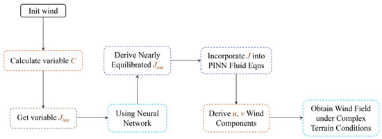
Figure 1.
The neural network model is utilized to compute the deformation characteristics of the flow field under complex terrain, represented by the deformation tensor J, during the diffusion process of the flow field, thereby inferring the wind field.
As shown in Figure 2, the PINN model employs neural network training to compute the iterative relationship between wind speed and air pressure, thereby obtaining the final wind field results. Conversely, the simplified model inherits the algorithmic process of using air pressure to calculate the wind field from the PINN model. However, the key distinction lies in the fact that the simplified model does not compute the final air pressure, pout, by iteratively calculating the relationship between the wind speed and air pressure. Instead, it utilizes neural networks to compute the variations in deformation tensors, consequently deriving the final air pressure, pout. Subsequently, the wind field under complex terrain conditions is inferred through deduction.
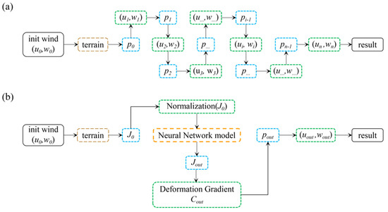
Figure 2.
(a) Computational flowchart of the PINN model; and (b) computational flowchart of the experimental model in this study.
The advantages of using the deformation tensor J to compute flow field variations include the following:
A. The value of the deformation tensor J is close to 1, while the deformation gradient C is close to 0. Computing the deformation gradient C is susceptible to interference from positive and negative signs and zeros, whereas using the deformation tensor J ensures numerical stability.
B. The spatial convection of the deformation tensor J adheres to physical laws. When air masses are compressed or stretched, deformation occurs, and the deformation tensor J exerts force on adjacent regions, thus generating a propagation mechanism.
C. The deformation of air masses results in changes in flow field characteristics. Using the deformation tensor J facilitates the convenient computation of flow field pressure gradients and wind speeds.
Compared to the PINN model, predicting diffusion through the deformation tensor J significantly simplifies the computational workload of the model.
2.3. Model Data Processing and Training Methods
The model adopts a Z-coordinate system and employs square grids to represent the terrain and air. Following the illustration in Figure 3, grid points in the flow field are labeled as either ‘terrain’ or ‘air mass’. After specifying the initial wind speed, the wind speed values at grid points labeled as ‘terrain’ are kept constant at 0.
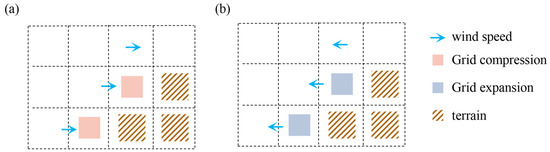
Figure 3.
The air mass is compressed near the terrain due to the influence of the wind field: (a) air mass compressed; and (b) air mass expanded.
Assuming deformation occurs not only in air grid points, but also in terrain grid points, as terrain points interact with air masses, deformation in the flow field generates stretching forces, and such deformation propagates from terrain grid points to nearby areas, forming a flow field adapted to the terrain. The deformation gradient C of the grid is computed using finite differences, as described in Equation (14).
According to Equation (7), the deformation gradient C is used to calculate the deformation parameter J0. Before inputting J0 into the neural network model, it undergoes normalization. Let Jinput = 0.5·J0, which is then used as the input layer of the model.
After undergoing processing by the neural network model, the variable Jinput yields the model training result Jnet. Subsequently, Jnet is subjected to reverse-normalization to obtain Jout = Jnet·2.
The computed deformation parameter Jout is substituted into Equations (10) and (11) to calculate the wind field adapted to the terrain features.
It should be noted that the deformation parameter J serves as the training output of the neural network model in this study. However, the deformation parameter Jout needs to be substituted into the fluid equations and the terrain-adapted wind field (uout, wout) computed. Subsequently, the terrain-adapted wind field (uout, wout) is utilized in training with the target wind field (u, w) to obtain the optimal solution of the neural network model. The training process is illustrated in Figure 4.
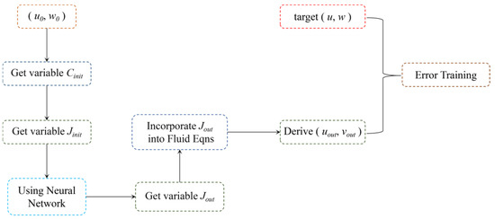
Figure 4.
Training flowchart.
There have been some achievements in simulating the spatial diffusion of physical quantities using convolution algorithms [34,35]. The “Using Neural Network” step mentioned in Figure 5 employs convolution algorithms, calculating the spatial diffusion of physical quantities through multi-level convolutions.
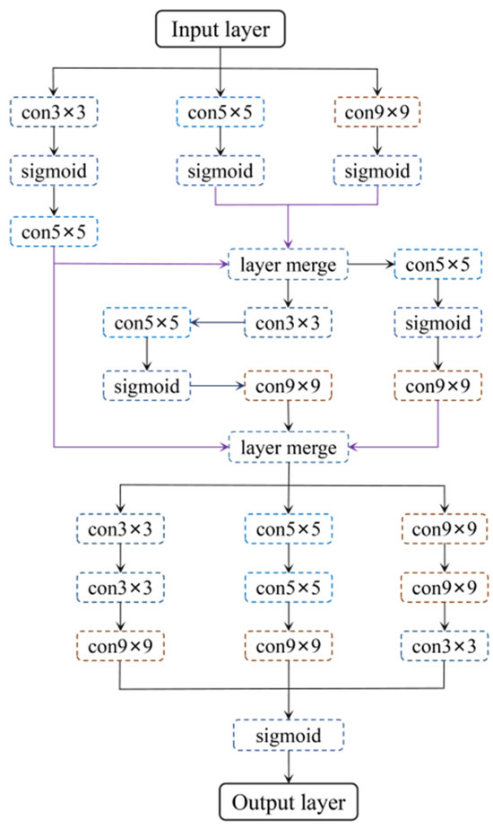
Figure 5.
The framework of the neural network model.
The advantage of convolution algorithms lies in their convenience in handling spatial relationships of physical quantities.
Figure 6 illustrates the operational process of a standard convolution. The convolution operation transfers and interacts with the data of neighboring grid points, achieving the spatial transfer of physical quantities.
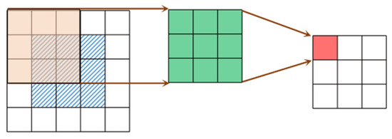
Figure 6.
The operational process of a standard convolution.
2.4. Source of Model Data
The experiment utilized terrain wind fields outputted by the Fluent model as a tool for model training. Fluent, as a powerful computational fluid dynamics simulation tool, effectively simulates and predicts atmospheric flow phenomena. Employing advanced algorithms and physical models, it accurately models the movement, propagation, and interaction of winds with other meteorological phenomena, providing crucial data support for meteorological forecasting.
Mainstream meteorological models, such as WRF, focus on mesoscale simulations with resolutions of typically up to 1 to 3 km. At grid spacings finer than 1 km, these models often underperform. In contrast, Fluent offers higher resolutions, accurately simulating terrain flow from 10 m to 500 m. Its precision is particularly noted in complex terrain airflow simulations. Therefore, Fluent is used by some researchers to dynamically downscale mesoscale models [36], aiming to enhance the wind field simulation accuracy and reliability.
2.4.1. Fluent Model Theory
In Fluent, the conservation equations for fluid mechanics problems consist of the mass conservation equation, momentum conservation equation, and energy conservation equation [37]. These equations can be expressed mathematically as follows [38]:
The mass conservation equation is as follows:
The momentum conservation equation is as follows:
The motion equation is as follows:
Here, u, v, and w represent the wind speeds in the x, y, and z directions, respectively, ρ represents the air density, and p represents the air pressure. The energy equation is as follows:
Here, E represents the system energy, μ represents the fluid viscosity coefficient, and Q represents the heat input.
Given the excellent performance of Fluent in atmospheric dynamic downscaling, this study employs the Fluent model to simulate wind field characteristics under complex terrain conditions and outputs wind fields close to steady-state conditions.
2.4.2. Terrain-Adapted Wind Field Data Output from Fluent Model
The advantage of the Fluent model lies in its ability to flexibly set initial wind fields and simulate wind fields adapted to terrain features.
As shown in Figure 7, a mountain range in the red box of area a is selected, and a 2D x–z section is extracted as the simulation area. Panel b displays the initial field set by Fluent, while panel c shows the adapted wind field output reflecting terrain characteristics. The model is configured for ‘steady-state simulation,’ where the term refers to assuming the characteristics of fluid flow remain constant throughout the simulation, disregarding the influence of time. In this simulation, parameters such as the fluid velocity field and pressure field may vary spatially, but their changes over time at any given point are negligible.
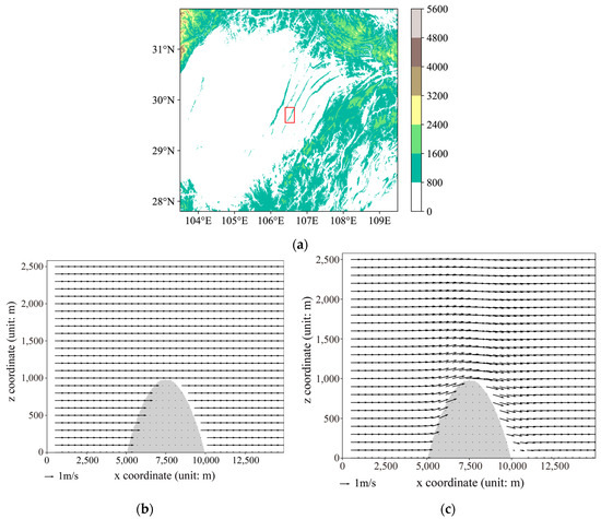
Figure 7.
(a)Target region: enclosed by the red boxt; (b) Initial wind field setting in Fluent; (c) wind field after adaptation to terrain.
Given the flexibility of the Fluent model in setting initial wind fields, the experimental design involved using Fluent to simulate terrain-adapted wind fields under specific terrain conditions and different initial wind speed states. Horizontal wind speeds were set at 1, 2, 3, …, 10 m/s, with an initial vertical velocity of 0. Corresponding terrain-adapted wind fields were obtained. Generally, the highest accuracy of the meteorological model resolution typically ranges from 400 m to 1 km. Therefore, in this study, Fluent model data with a higher precision were interpolated onto grid points with a resolution of 400 m to serve as training data for the neural network model, aiming to investigate methods for the dynamical downscaling of meteorological models.
The initial wind field settings in the Fluent model and the output terrain-adapted wind fields served as sample data, which were used as training data for the neural network model.
2.5. Error Evaluation Formula
The input data for the model are the initial wind field ( u0, w0 ) and terrain mask data.
The target data for model training are the wind field data obtained from Fluent calculations.
The error evaluation formula used for model training adopts the method outlined in Equation (21).
The MSE is used to evaluate the proximity between the model’s predicted values y’ and the true values y. During the training process, when the MSE error falls below the specified threshold and stabilizes, it can be considered that the model training is completed.
3. Results
In this study, based on the principle that wind speed perturbations induce ‘deformations’ in the fluid, we predict the overall disturbance characteristics of the terrain on the flow field using a neural network model. According to these characteristics, we employ a pressure gradient correction algorithm from fluid models to solve for the wind field situation after being perturbed by the terrain.
3.1. Training Performance of the Neural Network Model
In this study, terrain obstacles were introduced into wind fields without considering terrain conditions, as shown in Figure 8a. It was observed that a wind speed gradient (denoted as ∇·V) occurred between the airflow and the mountain obstacles. The velocity difference in the flow field causes fluid elements to be compressed or expanded, leading to the deformation of the fluid elements.
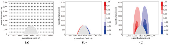
Figure 8.
(a) Initial wind field; (b) initial deformation characteristics corresponding to the initial wind field; and (c) deformation characteristics of the flow field after adaptation to terrain (obtained through training of the neural network model).
Due to the small magnitude of the deformation variable C, a normalization algorithm based on Equation (22) is employed in Figure 8b,c for better visualization.
Figure 8b illustrates the deformation characteristics of the flow field corresponding to the initial wind field, while Figure 8c illustrates the overall deformation characteristics of the flow field corresponding to the terrain-adapted wind field. From the figure, it can be observed that the flow field deformation closely follows the variations in topography.
3.2. Simulation of Terrain-Adapted Wind Fields
This section presents the training results of the neural network model and compares them with those of the Fluent model.
Figure 9 illustrates the results, taking an initial wind speed of 2 m/s as an example. Figure 9a shows the output results of the neural network model, while Figure 9b displays the computational results from Fluent. Both demonstrate good consistency, particularly in depicting physical phenomena such as airflow obstruction and forced lifting near the terrain. Although some differences exist near the surface of the terrain between the two models, overall, the influence of terrain on wind field disturbance is accurately represented in both sets of models and can propagate into higher altitudes.
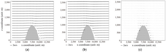
Figure 9.
At an initial wind speed of 2 m/s, (a) simulated results from the neural network model, (b) simulated results from Fluent, and (c) the difference between Fluent results and neural network model results.
As shown in Figure 10, when the initial wind speed is increased from 2 m/s to 5 m/s, the wind fields outputted by both the neural network model and the Fluent model maintain consistency in terms of regularity, with stable distributions of wind vectors. Through testing and validation, it has been confirmed that, within the wind speed range of 1 to 10 m/s, the overall distribution patterns of terrain-induced wind disturbances computed by these two models remain consistent.
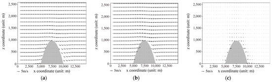
Figure 10.
At an initial wind speed of 5 m/s, (a) simulated results from the neural network model, (b) simulated results from Fluent, and (c) the difference between Fluent results and neural network model results.
3.3. Updraft Effect of Airflow
In terrain wind field models, the simulation of terrain-induced lifting in the wind field is an important metric in atmospheric modeling.
As shown in Figure 11, representative points are selected in the airspace above the windward slope, serving as ‘monitoring points’ and ‘monitoring lines’ to observe the vertical velocity changes near the monitoring points. These changes are used as evaluation indicators to validate the modeling capabilities of the neural network model.
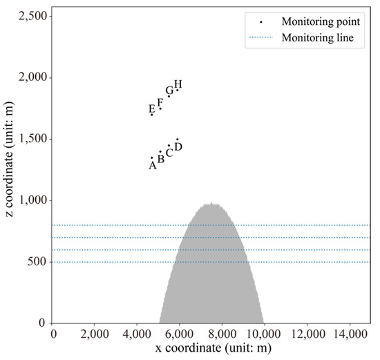
Figure 11.
Wind-speed-monitoring point above the windward slope.
Figure 12 compares the vertical wind speeds at each monitoring point between the two models under the same initial wind speed conditions. Upon observation of the bar chart, the results from both models exhibit close proximity. To further evaluate the computational outcomes, the calculation formulae for the root mean square error (RMSE) and mean absolute error (MAE) are introduced, as detailed in Equations (23) and (24), where (Wi*) represents the computed results from the neural network model and (Wi) denotes the corresponding results from the Fluent model [39].
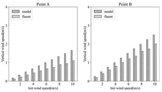
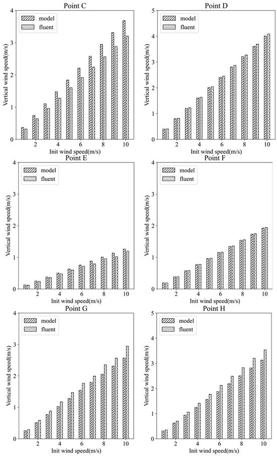
Figure 12.
Vertical velocity distribution at each monitoring point under different initial wind speed conditions. The horizontal axis represents the initial horizontal wind speed before inputting the model (Unit: m/s), and the vertical axis represents the vertical velocity (Unit: m/s). The sub-illustrations A to H are each associated with the respective monitoring points A to H, as indicated in Figure 11.
Table 1 presents the computed root mean square error (RMSE) and mean absolute error (MAE) results for each monitoring point, with “All” indicating the comprehensive RMSE across all monitoring points. From Table 1, it can be observed that both the RMSE and MAE values for the monitoring points fluctuate within the range of 0.1 to 0.35, indicating that the wind speed error deviations at each monitoring point are within reasonable limits.

Table 1.
Statistical performance metrics of the neural network model.
The results indicate that the neural network model’s ability to simulate the uplifting disturbance of the terrain on the airflow field can reach the simulation efficiency of the Fluent model, albeit with some degree of error. As the initial horizontal wind speed increases, the terrain uplifting effect strengthens, leading to an increase in the vertical wind speeds induced by terrain disturbances, which, in turn, amplifies the discrepancies between the two models.
In order to further investigate the vertical velocity distribution on both sides of the mountain, this study selects the vertical velocity distribution data at different altitudes (500 m, 600 m, 700 m, and 800 m) along the dashed lines as shown in Figure 13, and presents them in Figure 13 to assess the influence of terrain disturbances on the vertical velocity distribution under the condition of a horizontal initial velocity of 5 m/s. The research results show that, on the windward slope, the upward airflow motion strengthens as it approaches the slope surface, while, on the leeward slope, a significant downward airflow motion is observed near the leeward slope. It is noteworthy that the data output by the neural network model is generally consistent with the trend of the Fluent model, but there are some errors in the calculation results, indicating room for improvement.
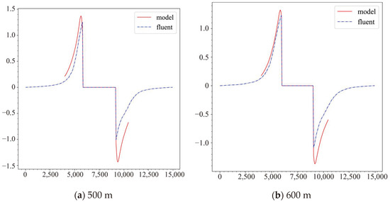
Figure 13.
Vertical velocity distribution at different height levels.
3.4. The Simulation Results Under Varied Terrain Conditions
To test the adaptability of the neural network model to changes in terrain, two sets of test experiments were added on top of the case results training:
- Adjust the position of the mountain in the horizontal translation case and observe the simulation results;
- Change the shape of the mountain in the case and observe the simulation results.
Taking 5 m/s as the initial wind speed, the author relocated the mountain’s center point from x = 7500 to x = 10,000. The wind field results were obtained through simulations using both the neural network model and Fluent model, and are visualized in Figure 14.
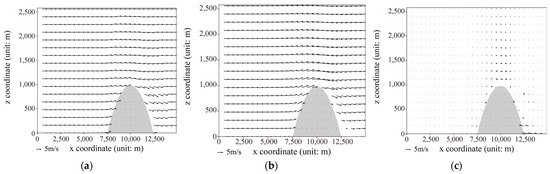
Figure 14.
The simulation results with an initial wind speed of 5 m/s: (a) neural network model simulation results; (b) Fluent model simulation results; and (c) Fluent results minus neural network model results.
In terms of simulating the upward airflow motion, the results of the neural network model are generally consistent with those of the Fluent tool. However, there is a certain simulation error on the leeward slope, which can be attributed to the tendency of airflow to generate turbulence on the leeward slope, a feature not yet incorporated into the neural network model. Nevertheless, it is worth emphasizing that the neural network model demonstrates a certain degree of adaptability to changes in terrain conditions.
Taking an initial wind speed of 5 m/s as an example, while keeping the central point of the mountain at x = 10,000 constant, a representative 2D terrain flow profile was re-extracted from the mountain range in Figure 7a. Simulations of the terrain flow field for this profile were subsequently conducted. The simulated results were then compared. For details of the terrain profile, please refer to Figure 15.
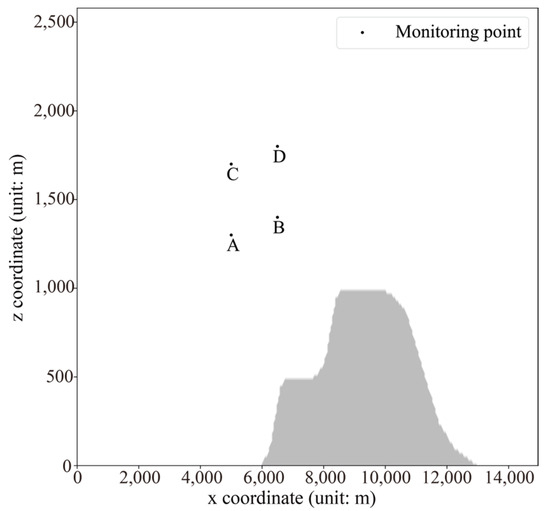
Figure 15.
Wind-speed-monitoring point above the windward slope.
In Figure 15, representative points are selected in the airspace above the windward slope as ‘monitoring points’ to observe the vertical velocity variations near these points. These variations serve as evaluation criteria to validate the generalization capability of the neural network model.
To verify the universality of the neural network model under various terrain conditions, detailed numerical simulations were conducted. As shown in Figure 16, altering the shape of the mountain resulted in the simulation of flow field characteristics using both the neural network model and Fluent tool. It was observed that significant turbulence occurred near the leeward slope when the shape of the mountain changed. Due to the limitations of the neural network model in simulating turbulence, there were certain deviations in the simulation results near the leeward slope compared to Fluent, but it could accurately simulate the airflow uplift process near the windward slope.
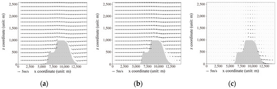
Figure 16.
Simulation of wind field after changes in mountain terrain shape, with an initial wind speed of 5 m/s: (a) neural network model simulation results; (b) Fluent model simulation results; and (c) Fluent results minus neural network model results.
Figure 17 depicts vertical wind speeds measured at various monitoring points, comparing differences between the two models under different initial wind speed conditions. The results indicate that vertical airflow velocities over terrain correlate positively with initial horizontal wind speeds. Numerical discrepancies exist between the two models in simulating updrafts, which amplify with increasing initial wind speeds.
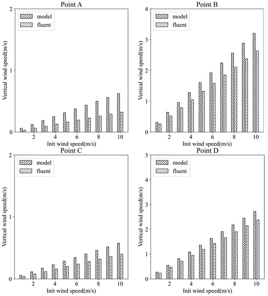
Figure 17.
Vertical velocity distribution at each monitoring point under different initial wind speed conditions. The horizontal axis represents the initial horizontal wind speed before inputting the model (Unit: m/s), and the vertical axis represents the vertical velocity (Unit: m/s). The sub-illustrations A to D are each associated with the respective monitoring points A to D, as indicated in Figure 15.
Table 2 presents the root mean square error (RMSE) and mean absolute error (MAE) data for each monitoring point, where “All” denotes the comprehensive RMSE across all monitoring points. From Table 2, it is observed that both the RMSE and MAE values for the monitoring points fluctuate within the range of 0.1 to 0.4, indicating that the model’s computed errors are within reasonable limits.
Table 2.
Statistical performance metrics of the neural network model.
In summary, despite altering the terrain shape, the neural network model can still accurately simulate airflow characteristics, demonstrating its ability to generalize.
3.5. The Computational Performance of the Model
To compare the computational speeds between Fluent and neural network models, we specifically recorded the computational times for a sample case. To validate the reliability of these times, both Fluent and the neural network models were tested on the same computer hardware (model: Xeon E5 2650) using a single-core CPU. The Fluent model, based on a C++ framework, reached equilibrium after approximately 500 iterations. We recorded the time consumption for iterations at 500, 1000, and 1500 cycles. The neural network model, based on a Python framework, averaged the time consumption across multiple simulations.
Table 3 summarizes the computational time consumption of two models under the terrain conditions corresponding to Figure 7c.
Table 3.
Time consumption under initial terrain conditions.
Table 3 reveals the neural network model’s shorter computation time compared to the Fluent tool’s for convergence using a single-core CPU, highlighting its immense potential for computational efficiency.
In Table 4, after altering terrain conditions, the Fluent model requires grid reconstruction, leading to changes in the model’s computation time.
Table 4.
Time consumption after changing the shape of the mountain.
From the time consumption in Table 3 and Table 4, we observe that the computation time of the Fluent model significantly increases when the terrain complexity changes. This is because Fluent needs to redraw the flow field grid to adapt to the new terrain conditions, resulting in an increased computational time as the terrain complexity and grid point numbers grow. In contrast, the neural network model employs a fixed square grid with consistent grid points, leading to minimal variation in computation time.
3.6. Limitations of the Research Papers
The neural network model employed in this study faced certain technical limitations during training. For instance, while the Fluent model utilized a high-density grid partitioning during the simulation, the neural network model employed a comparatively coarse grid, which somewhat diminished its simulation accuracy. Additionally, there were some technical imperfections as outlined below:
(I) Limitations of the training data
The model’s training data are derived from Fluent outputs corresponding to Figure 7c, with the training data having initial wind speeds of 2.5 m/s, 5.5 m/s, and 7.5 m/s, while the testing data range from 1 m/s to 10 m/s. The model is trained on a small subset of data and applied to compute a broader range of test data. This training approach may result in an insufficient representation of training samples.
(II) Limitations of the Fluent model
Compared to mainstream meteorological models like WRF, Fluent exhibits certain limitations in meteorological applications:
a. Fluent is suitable for simulating small-scale atmospheric flow and diffusion processes but may not be suitable for large- and medium-scale meteorological phenomena such as atmospheric circulation and weather systems.
b. While Fluent can simulate aspects of weather processes such as wind fields and the condensation of gaseous water into raindrops, it lacks the capability to simulate the entire weather process.
(III) Unconsidered influencing factors
Turbulence is typically generated on the leeward slope; however, due to the complexity and diversity of turbulence characteristics, the model in this study inadequately considers this important influencing factor, potentially leading to an insufficient predictive accuracy in certain scenarios.
4. Conclusions
In conclusion, addressing the challenges of atmospheric downscaling, terrain-adaptive wind fields, and convective weather warning simulations in complex terrains, this study introduces a deep-learning-based approach to simulate the atmospheric lifting process in such conditions and to apply these insights to the prediction of severe convective weather alerts. The innovations of this study are summarized as follows:
(I) This experiment innovatively extracts scalar data from the initial (u,w) wind field vector data as key training parameters, replacing direct training on wind vectors, thereby achieving the adaptive simulation of wind fields under complex terrain conditions. The advantage of this approach lies in avoiding direct vector training, reducing the training difficulty, and enhancing the model’s generalization ability.
(II) This experiment proposes using the fluid deformation variable J as the core parameter for model training. The variable J demonstrates good versatility in handling terrain grid points and fluid grid points, effectively reducing the difficulty of dealing with terrain grid points in the flow field. Compared to the deformation gradient C, the variable J avoids the complexity of positive and negative sign operations, thereby eliminating potential disturbances caused by positive and negative signs and zero operations during training. This further reduces the training difficulty of the fluid model and helps improve its generalization ability.
(III) Compared to traditional atmospheric dynamic modeling methods, the approach using neural network models in this study significantly reduces the complexity of modeling atmospheric flow fields. By capturing characteristic patterns of terrain conditions, it simulates wind field features in complex terrains, providing a new method and reference for addressing meteorological issues in complex terrain conditions.
Author Contributions
Conceptualization, X.W.; methodology, X.W.; software, X.W.; formal analysis, X.C; investigation, H.L.; resources, Y.L. and J.G.; data curation, X.C.; writing—original draft preparation, X.W.; writing—review and editing, J.G.; project administration, Y.L.; funding acquisition, Y.L. and J.G. All authors have read and agreed to the published version of the manuscript.
Funding
This research was funded by The National Natural Science Foundation of China—Research on response mechanism of micro terrain rainstorm and adaptive rainstorm flood forecasting method in areas with lack of data (Grant NO: 52109004), The National Key R&D Program of China (Grant NO: 2022YFC3002704), The National Key R&D Program of China (Grant NO: 2023YFC3209104), The National Key R&D Program of China (Grant NO: 2023YFC3209105), The National Key R&D Program of China (Grant NO: 2021YFC3200301), Project U2340211 supported by National Natural Science Foundation of China (Grant NO: U2340211), The Strategic Consulting Project supported by the Chinese Academy of Engineering (CAE) (Grant NO: HB2024C18), and The Fundamental Research Funds for the Central Universities (Grant NO: HUST:2024JYCXJJ020). Special thanks are extended to the editors and anonymous reviewers for their constructive comments.
Data Availability Statement
The data presented in this study are available upon request from the corresponding author. The data are not publicly available due to data copyright issues.
Conflicts of Interest
The authors declare no conflicts of interest.
References
- Ma, H.Y.; Ji, X.; Neelin, J.D.; Mechoso, C.R. Mechanisms for Precipitation Variability of the Eastern Brazil/SACZ Convective Margin. J. Clim. 2011, 24, 3445–3456. [Google Scholar] [CrossRef][Green Version]
- Makarieva, A.M.; Gorshkov, V.G.; Nefiodov, A.V.; Sheil, D.; Nobre, A.D.; Bunyard, P.; Nobre, P.; Li, B.-L. The equations of motion for moist atmospheric air. J. Geophys. Res. Atmos. 2017, 122, 7300–7307. [Google Scholar] [CrossRef]
- Heymsfield, A.J.; Sabin, R.M. Cirrus Crystal Nucleation by Homogeneous Freezing of Solution Droplets. J. Atmos. Sci. 1989, 46, 2252–2264. [Google Scholar] [CrossRef]
- Celik, F.; Marwitz, J.D. Droplet Spectra Broadening by Ripening Process. Part I: Roles of Curvature and Salinity of Cloud Droplets. J. Atmos. Sci. 2010, 56, 3091–3105. [Google Scholar] [CrossRef]
- Higgins, R.W.; Yao, Y.; Yarosh, E.S.; Janowiak, J.E.; Mo, K.C. Influence of the Great Plains Low-Level Jet on Summertime Precipitation and Moisture Transport over the Central United States. J. Clim. 1997, 10, 481–507. [Google Scholar] [CrossRef]
- Wei, X.; Liu, Y.; Guo, J.; Chang, X.; Li, H. Applicability Study of Euler—Lagrange Integration Scheme in Constructing Small-Scale Atmospheric Dynamics Models. Atmosphere 2024, 15, 644. [Google Scholar] [CrossRef]
- Landel, G.; Smith, J.A.; Baeck, M.L.; Steiner, M.; Ogden, F.L. Radar studies of heavy convective rainfall in mountainous terrain. J. Geophys. Res. Atmos. 1999, 104, 31451. [Google Scholar] [CrossRef]
- Baik, J.-J.; Park, S.-B. Urban Flow and Dispersion Simulation Using a CFD Model Coupled to a Mesoscale Model. J. Appl. Meteorol. Climatol. 2009, 48(8), 1667–1681. [Google Scholar] [CrossRef]
- Schlager, C.; Kirchengast, G.; Fuchsberger, J.; Kann, A.; Truhetz, H. A spatial evaluation of high-resolution wind fields from empirical and dynamical modeling in hilly and mountainous terrain. Geosci. Model Dev. 2019, 12, 2855–2873. [Google Scholar] [CrossRef]
- Poulsen, T.; Niclasen, B.A.; Giebel, G.; Beyer, H.G. Validation of WRF generated wind field in complex terrain. Meteorol. Z. 2021, 30, 413–428. [Google Scholar] [CrossRef]
- Luo, X.; Cao, Y. Simulation of the wind fields over complex terrain with coupling of CFD and WRF. J. Comput. Methods Sci. Eng. 2021, 21, 1155–1166. [Google Scholar] [CrossRef]
- Li, S.; Sun, X.; Zhang, S.; Zhao, S.; Zhang, R. A Study on Microscale Wind Simulations with a Coupled WRF–CFD Model in the Chongli Mountain Region of Hebei Province, China. Atmosphere 2019, 10, 731. [Google Scholar] [CrossRef]
- Martynova, Y.V.; Zaripov, R.B.; Krupchatnikov, V.N.; Petrov, A.P. Estimation of the quality of atmospheric dynamics forecasting in the siberian region using the wrf-arw mesoscale model. Russ. Meteorol. Hydrol. 2014, 39, 440–447. [Google Scholar] [CrossRef]
- Chan, P.W.; Lam, C.C.; Cheung, P. Numerical simulation of wind gusts in intense convective weather and terrain-disrupted airflow. Atmósfera 2011, 24, 287–309. [Google Scholar] [CrossRef][Green Version]
- Codiga, D.L.; Cornillon, P. Effects of Geographic Variation in Vertical Mode Structure on the Sea Surface Topography, Energy, and Wind Forcing of Baroclinic Rossby Waves. J. Phys. Oceanogr. 2003, 33, 1219–1230. [Google Scholar] [CrossRef]
- Guo, J.; Liu, Y.; Zou, Q.; Ye, L.; Zhu, S.; Zhang, H. Study on optimization and combination strategy of multiple daily runoff prediction models coupled with physical mechanism and LSTM. J. Hydrol. 2023, 624, 129969. [Google Scholar] [CrossRef]
- Chang, X.; Guo, J.; Qin, H.; Huang, J.; Wang, X.; Ren, P. Single-Objective and Multi-Objective Flood Interval Forecasting Considering Interval Fitting Coefficients. Water Resour. Manag. 2024, 38, 3953–3972. [Google Scholar] [CrossRef]
- Guo, J.; Xu, X.J.; Lian, W.W.; Zhu, H.L. A new approach for interval forecasting of photovoltaic power based on generalized weather classification. Int. Trans. Electr. Energy Syst. 2019, 29, e2802. [Google Scholar] [CrossRef]
- Ren, P.; Rao, C.; Liu, Y.; Wang, J.-X.; Sun, H. PhyCRNet: Physics-informed convolutional-recurrent network for solving spatiotemporal PDEs. Comput. Methods Appl. Mech. Eng. 2022, 389, 114399. [Google Scholar] [CrossRef]
- Zhang, F.; Lai, C.; Chen, W. Weather Radar Echo Extrapolation Method Based on Deep Learning. Atmosphere 2022, 13, 815. [Google Scholar] [CrossRef]
- Manero, J.; Béjar, J.; Cortés, U. Deep Learning is blowing in the wind. Deep models applied to wind prediction at turbine level. J. Phys. Conf. Ser. 2019, 1222, 012037. [Google Scholar] [CrossRef]
- Yu, T.; Yang, R.; Huang, Y.; Gao, J.; Kuang, Q. Terrain-Guided Flatten Memory Network for Deep Spatial Wind Downscaling. IEEE J. Sel. Top. Appl. Earth Obs. Remote Sens. 2022, 15, 9468–9481. [Google Scholar] [CrossRef]
- Guo, J.; Feng, T.; Cai, Z.L.; Lian, X.L.; Tang, W.H. Vulnerability Assessment for Power Transmission Lines under Typhoon Weather Based on a Cascading Failure State Transition Diagram. Energies 2020, 13, 3681. [Google Scholar] [CrossRef]
- Qiao, D.; Wu, S.; Li, G.; You, J.; Zhang, J.; Shen, B. Wind speed forecasting using multi-site collaborative deep learning for complex terrain application in valleys. Renew. Energy 2022, 189, 231–244. [Google Scholar] [CrossRef]
- Afzali, J.; Casas, C.Q.; Arcucci, R. Latent GAN: Using a Latent Space-Based GAN for Rapid Forecasting of CFD Models. In 21st International Conference on Computational Science; Springer: Cham, Switzerland, 2021; Volume 12746, pp. 360–372. [Google Scholar]
- Khan, M.; Naeem, M.R.; Al-Ammar, E.A.; Ko, W.; Vettikalladi, H.; Ahmad, I. Power Forecasting of Regional Wind Farms via Variational Auto-Encoder and Deep Hybrid Transfer Learning. Electronics 2022, 11, 206. [Google Scholar] [CrossRef]
- Chen, H.; Birkelund, Y.; Zhang, Q. Data-augmented sequential deep learning for wind power forecasting. Energy Convers. Manag. 2021, 248, 114790. [Google Scholar] [CrossRef]
- Zhang, W.; Hranilovic, S.; Shi, C. Soft-switching hybrid FSO/RF links using short-length raptor codes: Design and implementation. IEEE J. Sel. Areas Commun. 2009, 27, 1698–1708. [Google Scholar] [CrossRef]
- Salameh, T.; Drobinski, P.; Vrac, M.; Naveau, P. Statistical downscaling of near-surface wind over complex terrain in southern France. Meteorol. Atmos. Phys. 2009, 103, 253–265. [Google Scholar] [CrossRef]
- Tang, Z.; Chang, X.; Ni, X.; Xiao, W.; Liu, H.; Guo, J. Evaluation Method of Severe Convective Precipitation Based on Dual-Polarization Radar Data. Water 2024, 16, 1136. [Google Scholar] [CrossRef]
- Shun, C.M.; Lau, S.Y.; Lee, O.S.M. Terminal Doppler Weather Radar Observation of Atmospheric Flow over Complex Terrain during Tropical Cyclone Passages. J. Appl. Meteorol. 2003, 42, 1697–1710. [Google Scholar] [CrossRef]
- Grell, G.A.; Dudhia, J.; Stauffer, D.R. A Description of the Fifth-Generation Penn State/NCAR Mesoscale Model (MM5); Technical Report NCAR/TN-398+STR; National Center for Atmospheric Research: Boulder, CO, USA, 1994. [Google Scholar]
- Qin, H.; Liu, J.; Xiao, J.; Zhang, R.; He, Y.; Wang, Y.; Sun, Y.; Burby, J.W.; Ellison, L.; Zhou, Y. Canonical symplectic particle-in-cell method for long-term large-scale simulations of the Vlasov-Maxwell system. J. Aerosp. Power 2015, 2071, 376–381. [Google Scholar] [CrossRef]
- Xu, J.Z.; Zhang, H.R.; Cheng, Z.; Liu, J.Y.; Xu, Y.Y.; Wang, Y.C. Approximating Three-Dimensional (3-D) Transport of Atmospheric Pollutants via Deep Learning. Earth Space Sci. 2022, 9, e2022EA002338. [Google Scholar] [CrossRef]
- Zhang, B.; Wang, Z.; Lu, Y.; Li, M.-Z.; Yang, R.; Pan, J.; Kou, Z. Air Pollutant Diffusion Trend Prediction Based on Deep Learning for Targeted Season—North China as an Example. Expert Syst. Appl. 2023, 232, 120718. [Google Scholar] [CrossRef]
- Zheng, Y.; Miao, Y.; Liu, S.; Chen, B.; Zheng, H.; Wang, S. Simulating Flow and Dispersion by Using WRF-CFD Coupled Model in a Built-Up Area of Shenyang, China. Adv. Meteorol. 2015, 2015, 1–15. [Google Scholar] [CrossRef]
- Sharma, P.K.; Warudkar, V.; Ahmed, S. Application of a new method to develop a CFD model to analyze wind characteristics for a complex terrain. Sustain. Energy Technol. Assess. 2020, 37, 100580. [Google Scholar] [CrossRef]
- Balogh, M.; Parente, A.; Benocci, C. RANS simulation of ABL flow over complex terrains applying an Enhanced k-epsilon model and wall function formulation: Implementation and comparison for fluent and OpenFOAM. J. Wind. Eng. Ind. Aerodyn. 2012, 104, 360–368. [Google Scholar] [CrossRef]
- Sunaid, K.; Khan, A.U.; Khan, M.; Khan, F.A.; Khan, S.; Khan, J. Intercomparison of SWAT and ANN techniques in simulating streamflows in the Astore Basin of the Upper Indus. Water Sci. Technol. 2023, 88, 1847–1862. [Google Scholar]


Disclaimer/Publisher’s Note: The statements, opinions and data contained in all publications are solely those of the individual author(s) and contributor(s) and not of MDPI and/or the editor(s). MDPI and/or the editor(s) disclaim responsibility for any injury to people or property resulting from any ideas, methods, instructions or products referred to in the content. |
© 2024 by the authors. Licensee MDPI, Basel, Switzerland. This article is an open access article distributed under the terms and conditions of the Creative Commons Attribution (CC BY) license (https://creativecommons.org/licenses/by/4.0/).