Hydrodynamic Porosity: A New Perspective on Flow through Porous Media, Part II

Abstract

In this work, we build upon our previous finding that hydrodynamic porosity is an exponential function of pore-scale flow velocity (or interstitial Reynolds number). We previously discovered this relationship for media with a square cavity geometry—a highly idealized case of the dead-ended pore spaces in a porous medium. Thus, we demonstrate the applicability of this relationship to media with other cavity geometries. We do so by applying our previous analysis to rectangular and non-rectangular cavity geometries (i.e., circular, and triangular). We also study periodic flow geometries to determine the effect of upstream cavities on those downstream. We show that not only does our exponential relationship hold for media with a variety of cavity geometries, but it does so almost perfectly with a coefficient of determination (R²) of approximately one for each new set of simulation data. Given this high fit quality, it is evident that the exponential relationship we previously discovered is applicable to most, if not all, unwashed media.

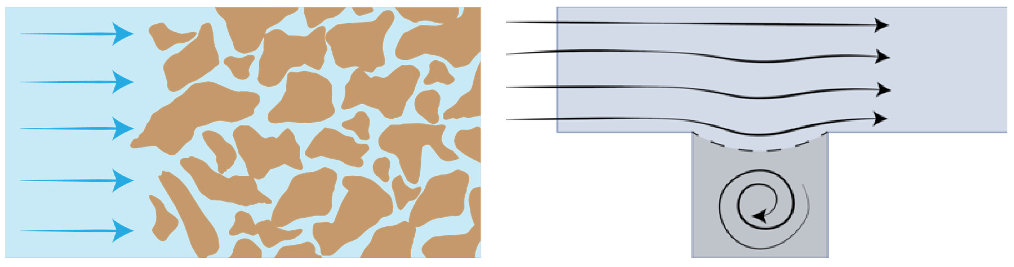
1. Introduction

Fluid flow and transport through porous media is important in nature and many engineered systems. Understanding pore-scale flow dynamics helps elucidate fluid transport mechanisms within porous media on macroscales.

The literature on the role of porosity in flow and transport through porous media and fractured rock has continued to grow over the last few decades—see review articles by Worthington [1], Yan et al. [2], and Meier et al. [3] and research articles by Coats and Smith [4], Yuan and Rezaee [5], Li et al. [6], Foroughi et al. [7], Verbovšek [8], Fenni et al. [9], Kango et al. [10], and Yao et al. [11].

As discussed in more detail in our companion (by Young and Kabala [12]), in porous media studies, the pore space is typically decomposed into two regions: mobile and “immobile” zones, as described by van Genuchten and Wierenga [13]. In the mobile zone, solute transport occurs via advection and dispersion. In the immobile zone consisting of isolated or dead-end pores (cavities), fluid is immobile or it recirculates in eddies, whereas solute transport is driven by molecular or vortex-enhanced diffusion.

In this paper, we build on our previous findings, i.e., Young and Kabala [12], where we discovered and quantified the exponential dependence of hydrodynamic porosity on pore-scale flow velocity or interstitial Reynolds number. This relationship is reproduced below:

$${\theta }_{mobile}=\left(a+b{e}^{-c{v}_{pore}}\right)\theta ⟺ {\theta }_{mobile}=\left(a+b{e}^{-dR}\right)\theta , where d={\displaystyle \frac{c height}{\nu }}$$

(1)

where ${\theta }_{mobile}$ is the mobile-zone porosity (i.e., what we refer to as the hydrodynamic porosity of the medium), $\theta$ is the total porosity of the medium, $height$ is the height of the through-channel in the dead-end pore model (m), $\nu$ is the kinematic viscosity (m²/s), and a, b, and d are dimensionless parameters; the exponential parameter, c, has units of s/m to allow for the use of pore-scale velocity in place of the Reynolds number. Readers are further reminded that a is the value of the pore-scale partitioning coefficient ($\xi$) approximated by the boundary-driven, or analogously, mobile–immobile zone model, both of which are discussed at length by Young and Kabala [12] and were originally applied to groundwater flows by Vangenuchten and Wierenga [13]. In the case of the mobile separatrix we study here, it is the value that results from Re $\to \infty$. Finally, the quantity ‘a + b’, is the value of $\xi$ in the creeping flow regime (i.e., the value that results from Re $\to 0$).

Equation (1) was discovered and quantified for the dead-end pore geometry reproduced in Figure 1, below. Readers will note that the cavity geometry is square. Thus, we did not previously determine if this relationship holds for more than this single idealized case. This work is motivated by the fact that the dead-ended pore spaces in unwashed porous media (e.g., glacial deposits, fractured rock, and filtration media such as granulated activated carbon, etc.) are poorly approximated by the square cavity geometry we previously studied. The jagged edges of such media result in a random array of pore geometries (as illustrated below). Subsequently, we must be able to answer the question: does the exponential dependence of hydrodynamic porosity on pore-scale flow velocity hold for media with cavity geometries that are not square? If the answer is indeed yes, researchers are justified in utilizing the exponential relationship provided in Equation (1) to better understand flow and transport in porous media.

2. Related Work

2.1. Flows Past Cavities

In our previous work, we provide a thorough literature review of flows past cavities, citing the major contributions that have led to a comprehensive understanding of cavity vortex structure(s), e.g., Moffatt [14]; Higdon [15]; Shen and Floryan [16]; Fang et al. [17]. Readers are directed to this discussion for further detail. In the following table, we summarize the popular cavity geometries studied by these (and other) authors. Following the precedent set by these authors, we proceed by utilizing analogous cavity geometries in our analysis.

Table 1. Geometries used in the study of flows past cavities.

Cavity Geometry
Rectangular	Non-Rectangular	Periodic
Young and Kabala [12] Kahler and Kabala [21] Moffatt [14] Mehta and Lavan [18] O’Brien [19] Shen and Floryan [16] Kang and Chang [22] Fang et al. [17] Higdon [15] Alkire et al. [23] Horner et al. [24]	Moffatt [14] Higdon [15] O’Neill [20]	Kahler and Kabala [21] Kang and Chang [22]

illustrates that most research has been carried out on rectangular cavity geometries. This is unsurprising given that sharp corners in flow geometries result in flow separation. Higdon [15], Shen and Floryan [16], Fang et al. [17], and Mehta and Lavan [18], O’Brien [19] utilize rectangular geometries and manipulate the cavity width and/or depth to determine the subsequent effect on the cavity vortex structure. Moffatt [14], in his study on resistive eddies that result from sharp corners, focuses most of his work on triangular structures, whereas Higdon [15] and O’Neill [20] study circular cavities.

2.2. Pore-Scale Flow Modeling

As discussed in more detail by Young and Kabala [12], we are numerically solving in Wolfram Language (Mathematica) the steady-state Navier–Stokes equation for incompressible Newtonian fluid (water) subject to no-slip and no-penetration boundary conditions on the walls of the channel and cavity. The pressure is specified at the outlet and the inlet velocity distribution is parabolic, as in a fully developed channel flow.

$${\displaystyle 𝛻}\cdot u=0$$

$$\rho \left(u\cdot \nabla u\right)=-\nabla p+\mu {\nabla }^{2}u$$

$$u\left(\left(x,y\right)=wall\right)=0$$

$$p\left(x=channel length,y\right)=0$$

where u is a 2D velocity vector, ρ is density, p is pressure, and μ is dynamic viscosity. Because we do not refer to these equations later, we list them unnumbered.

As in our companion paper (Young and Kabala [12]), we assume steady-state, laminar flow, as typically encountered in ambient groundwater as well as in pump-and-treat remediation conducted with a constant pumping rate. The ambient flows with the Reynolds numbers Re = $R$ < 1 are laminar and so are forced-gradient flows, which typically do not exceed the particle-size-based Reynolds numbers Re = $R$ < 100, even near a pumping well. For our numerical experiments, we chose Reynolds numbers that span this laminar range—see further discussion in our companion paper (Young and Kabala [12]).

We conducted convergence analysis to decide on the suitable refinement of the numerical grid. It is included in the Supplementary Materials. As shown there and in the Wolfram Numerical Solution of Partial Differential Equations [25], our numerical errors related to finite-element discretization do not exceed 2% and are likely significantly smaller.

Many articles deal with flow over cavities and present numerical and experimental results analogous to ours. Although none of them introduce and study the concept of hydrodynamic porosity, their results confirm our findings at least qualitatively. Some are numerical (e.g., Takematsu [26]; Friedman [27]; Stevenson [28]; O’Brien [19]; Higdon [15]; and Driesen et al. [29]), some are experimental (e.g., Taneda [30]; Shankar and Deshpande [31]; Laskowska [32]), and some are mixed (e.g., Shen and Florian [16]; Pan and Acrivos [33]).

2.3. Our Previous Work

The idealized, square cavity geometry we previously utilized in Young and Kabala [12] is justified by its foundational use in the study of flows past cavities and is included in most of the studies referenced in Table 1 above. To exaggerate the dependence of hydrodynamic porosity on pore velocity, we also narrowed the height of the through-channel, relative to the cavity depth and width, which is kept at a one-to-one aspect ratio so that the cavity remains square; readers are referred to Figure 6 of Young and Kabala [12] for reference.

We then subjected these dead-end pore geometries to inlet flows with an interstitial (channel-based) Reynolds number in the range of 1–100, reasoning that doing so keeps the flow within the laminar regime. To justify this claim, we reference multiple examples that demonstrate a general trend: the onset of turbulence occurs at or above Reynolds numbers of 100 in porous media, e.g., Jolls and Hanratty [34]; Wegner et al. [35]; Latifi et al. [36]; Rode et al. [37]; Bu et al. [38], etc. For each dead-end pore geometry, we discovered an exponential dependence of hydrodynamic porosity on pore-scale flow velocity, with a coefficient of determination (R²) of approximately one for each set of simulation data. As anticipated, this relationship was most exaggerated when the through-channel height of the dead-end pore geometry was reduced to one-quarter of the cavity depth/width. For media with this cavity type, the hydrodynamic porosity decreased by 42% over the laminar flow regime. For reference, over the same Reynolds number range, the hydrodynamic porosity only decreased by 4% when the through-channel height was equivalent to the cavity depth/width.

3. Methods

In short, the hydrodynamic porosity of a porous medium with dead-ended pore spaces is ultimately determined by the location of the separatrix (i.e., the streamline that divides the through-channel flow from the recirculatory cavity flow), which we track over a range of flow conditions by varying the magnitude of the interstitial Reynolds number of the inlet flow. Further discussion on the separatrix is provided by (Elderkin [39]; Weiss [40]; Horner et al. [24]; Kahler and Kabala [18]). We track the location of the separatrix because it defines the magnitude of the mobile zone (i.e., the pore space conducive to through-flow), and therefore the value of the pore-space partitioning coefficient ($\xi$):

$$\xi ={\displaystyle \frac{V_{mobile}}{V_{pore}}}={\displaystyle \frac{A_{mobile}}{A_{pore}}}$$

(2)

As defined above, the pore-space partitioning coefficient is the ratio of the mobile-zone volume ($V_{mobile})$ to the total pore space volume ($V_{pore}$). For an isotropic, or 2D media, like the ones we study in this work, $\xi$ can be defined in terms of cross-sectional areas, $A$. The product of the total porosity of the medium and the partitioning coefficient yield the hydrodynamic porosity (${\theta }_{mobile}$) of the medium:

$${\theta }_{mobile}=\xi \theta$$

(3)

The methods and tools used in this analysis are the same as those used in our previous work. Readers are directed to Young and Kabala [12] for a description of the numerical flow solver we leverage in this analysis, as well as a detailed outline of the data collection process. Slight modifications to the flow solver program allow for manipulation of the cavity geometry, which we picture in the figures below. With each cavity manipulation, we adjust the refinement region of the solver mesh to fully encapsulate the area in which we assume the separatrix to be. Altogether, we test rectangular cavities with depth-to-width ratios of 2:1, 1.5:1, 1:1, and 0.5:1 (pictured in Figure 2), and 1:2, 1:1.5, 1:1, and 1:0.5 (pictured in Figure 3). The varying channel length in the geometries provided in Figure 3 is an artifact of the decision to extend the length of the through-channel past the cavity by twice the cavity width. We also test two non-rectangular cavities (i.e., a semicircle and an equilateral triangle). Finally, we test periodic flow geometry to determine the effect upstream cavities have on those downstream. These additional flow geometries are provided below, in Figure 4 and Figure 5.

Again, these flow geometries are subjected to an inlet flow with channel-based Reynolds numbers in the laminar flow regime (i.e., Re < 100). For ease of comparison to our previous results, we determine the location of the separatrix at the same Reynolds numbers (i.e., Re = 1.81, 3.61, 5.52, 9.19, 25, 50, 75, 100). Note that we do not test Reynolds numbers in the creeping flow regime, which in this case, is less than 1. This is because we previously found that the separatrix is immobile in this regime (Young and Kabala [12]). After having subjected each flow geometry to the specified Reynolds numbers, we apply the exponential relationship in Equation (1) that we discovered for the square cavity geometry to each new set of simulation data. We determine the fit quality of the exponential model via the coefficient of determination (R²). Finally, given the sparse sampling we previously used to generate the exponential relationship we define in Equation (1), we also determine the error associated with this low sampling frequency; we do this by testing Reynolds numbers of 1–100 in increments of 5.

4. Results

Stream plots for each cavity geometry at Reynolds numbers of approximately 1, 10, 50, and 100, are provided in the figures below. In each stream plot, the separatrix is highlighted in red. Again, because the cavity flow is driven by the adjacent through-channel flow, we also provide a stream plot of the entire flow geometry adjacent to the corresponding cavity flow. Figure 6 below is reproduced from our previous work.

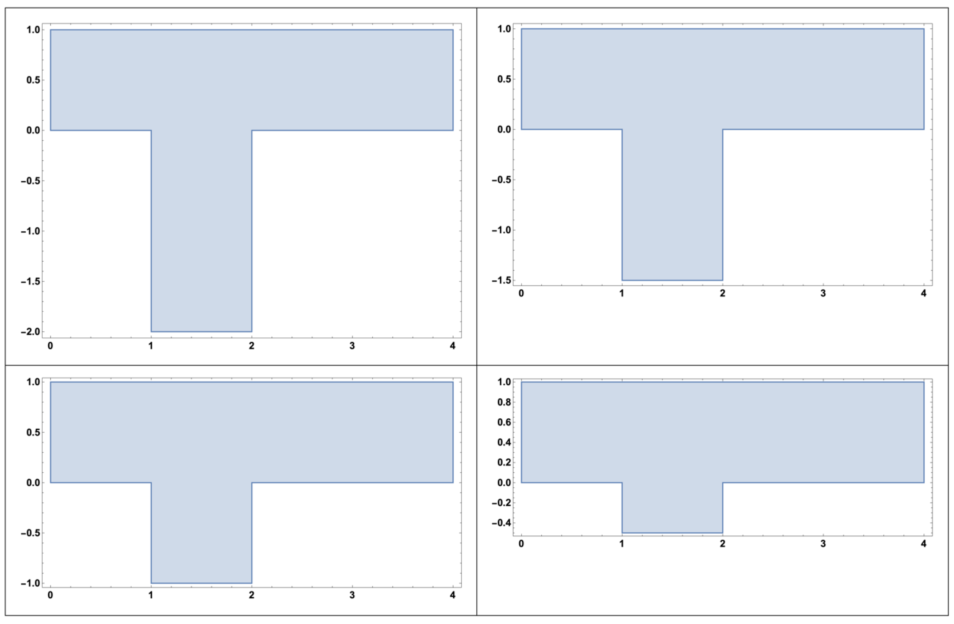
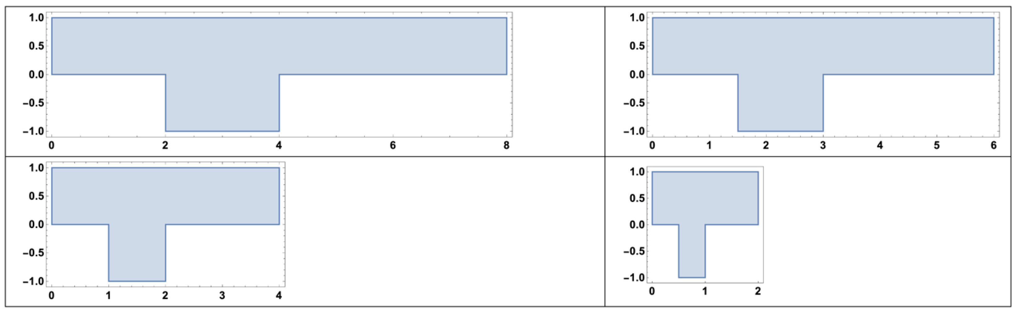
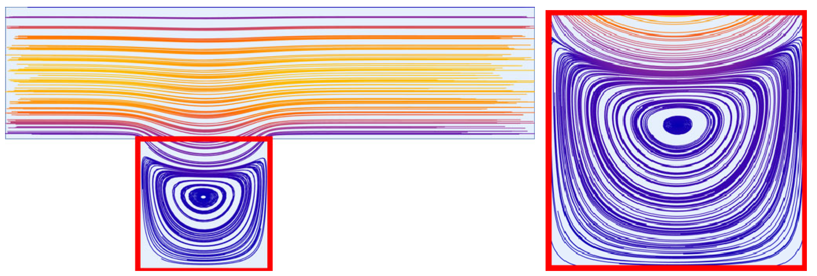
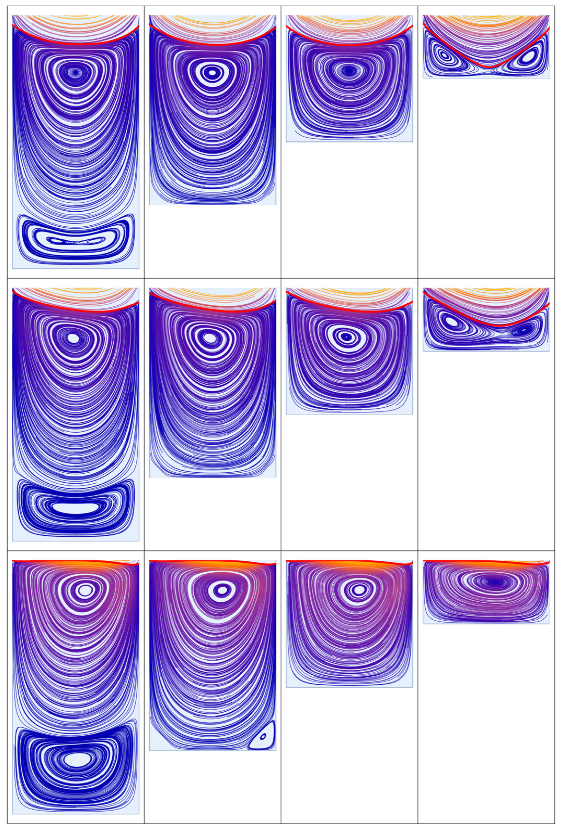
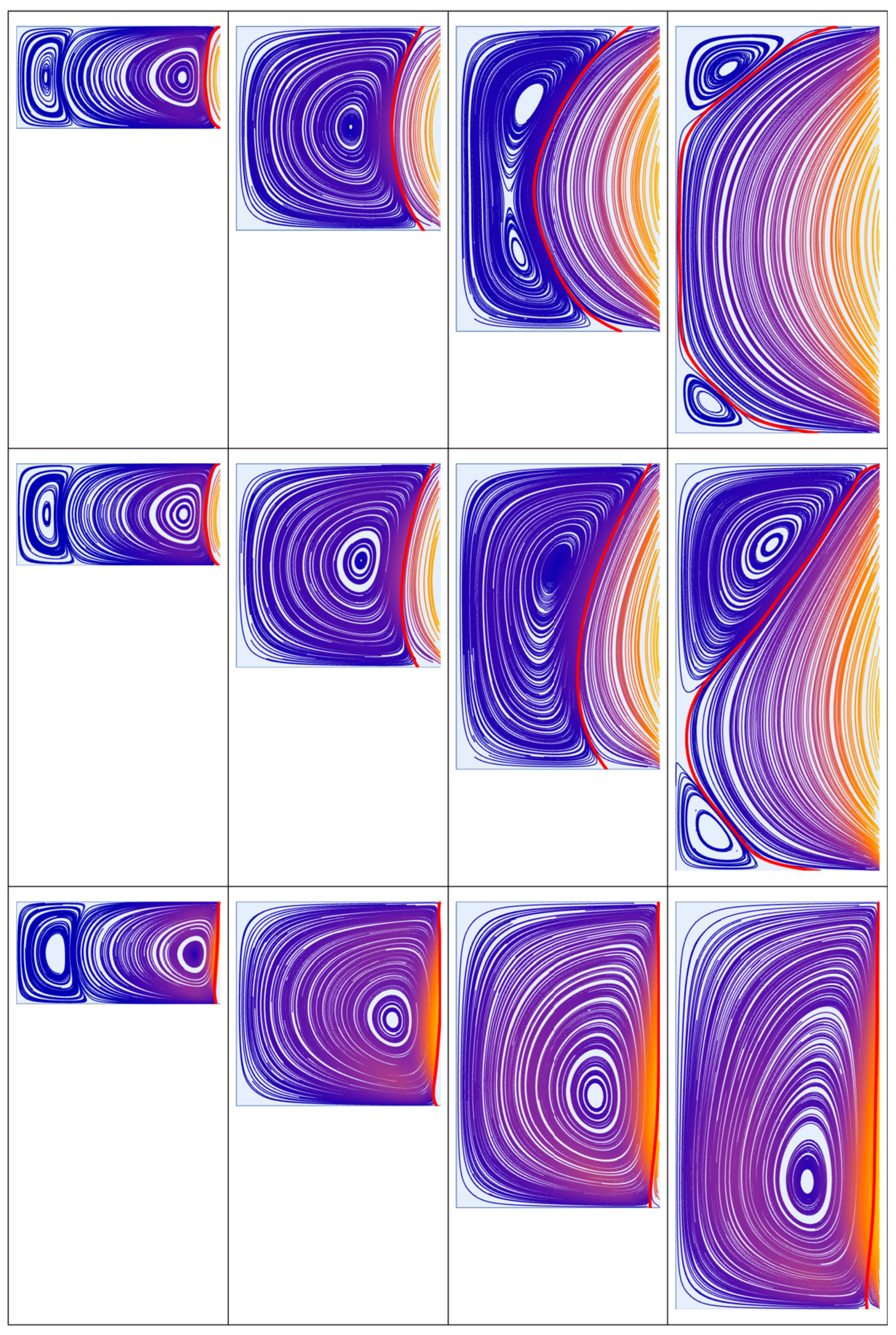
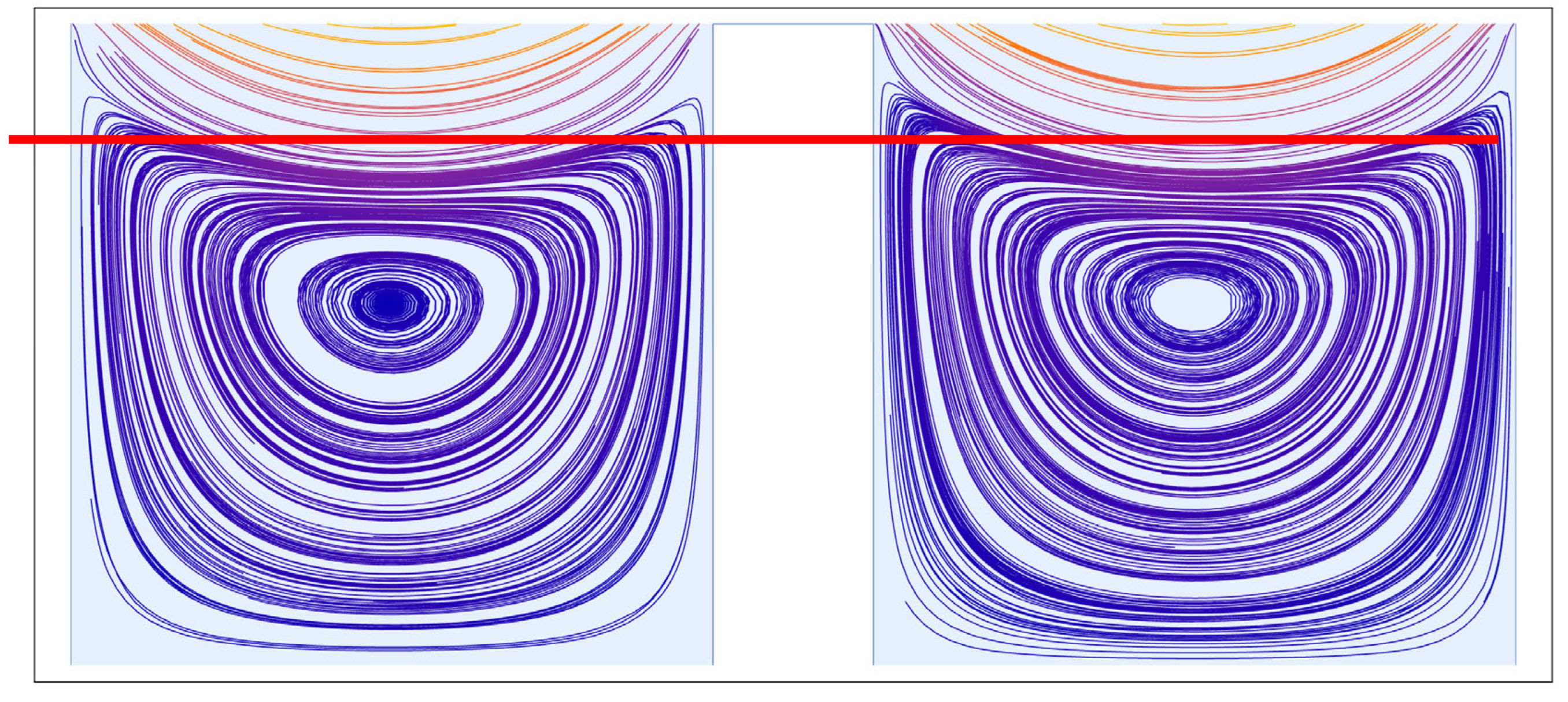
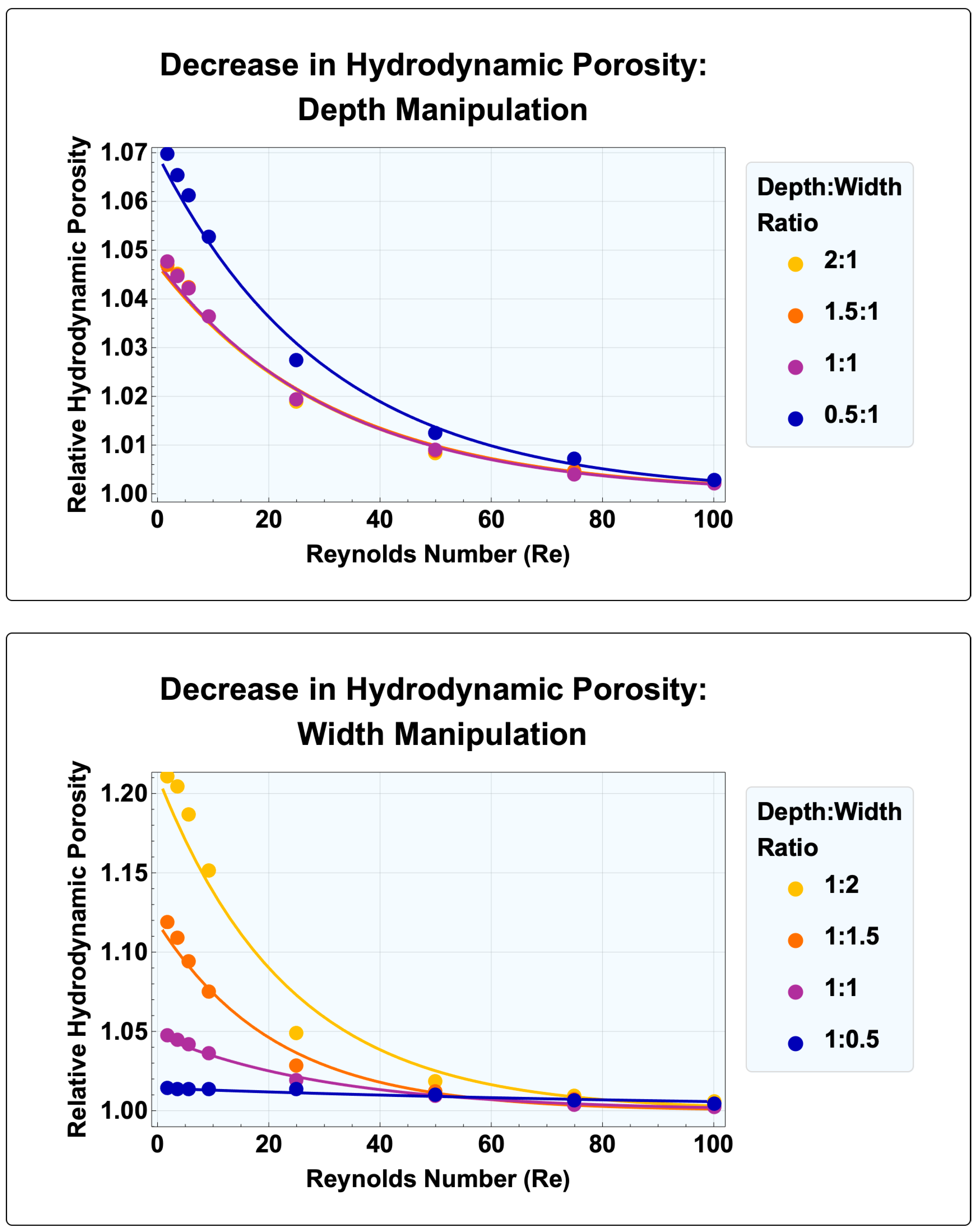
4.1. Separatrix Movement: Rectangular Cavity Geometry Manipulation

In Figure 7, Figure 8, Figure 9 and Figure 10 below, we provide the stream plots that result when we adjust the depth and width of the square cavity geometry we previously tested. We also illustrate the movement of the separatrix, which is highlighted in red.

Separatrix movement, as a function of Reynolds number, is summarized in the figures below. In each figure, the separatrix is highlighted according to its location at a given Reynolds number (yellow, orange, red, and blue for Reynolds numbers 1.81, 9.19, 50, and 100, respectively).

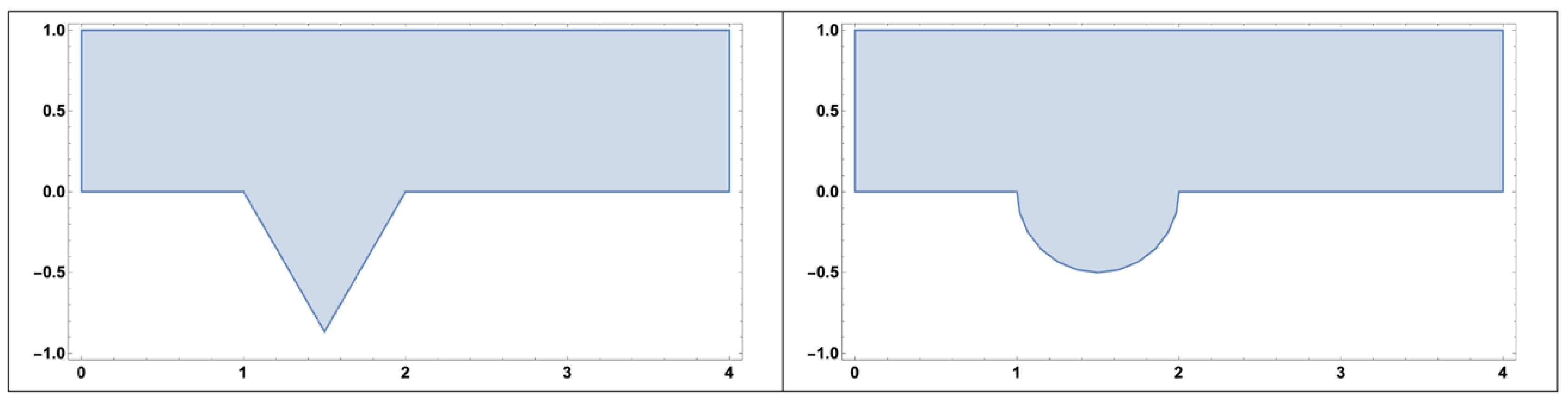
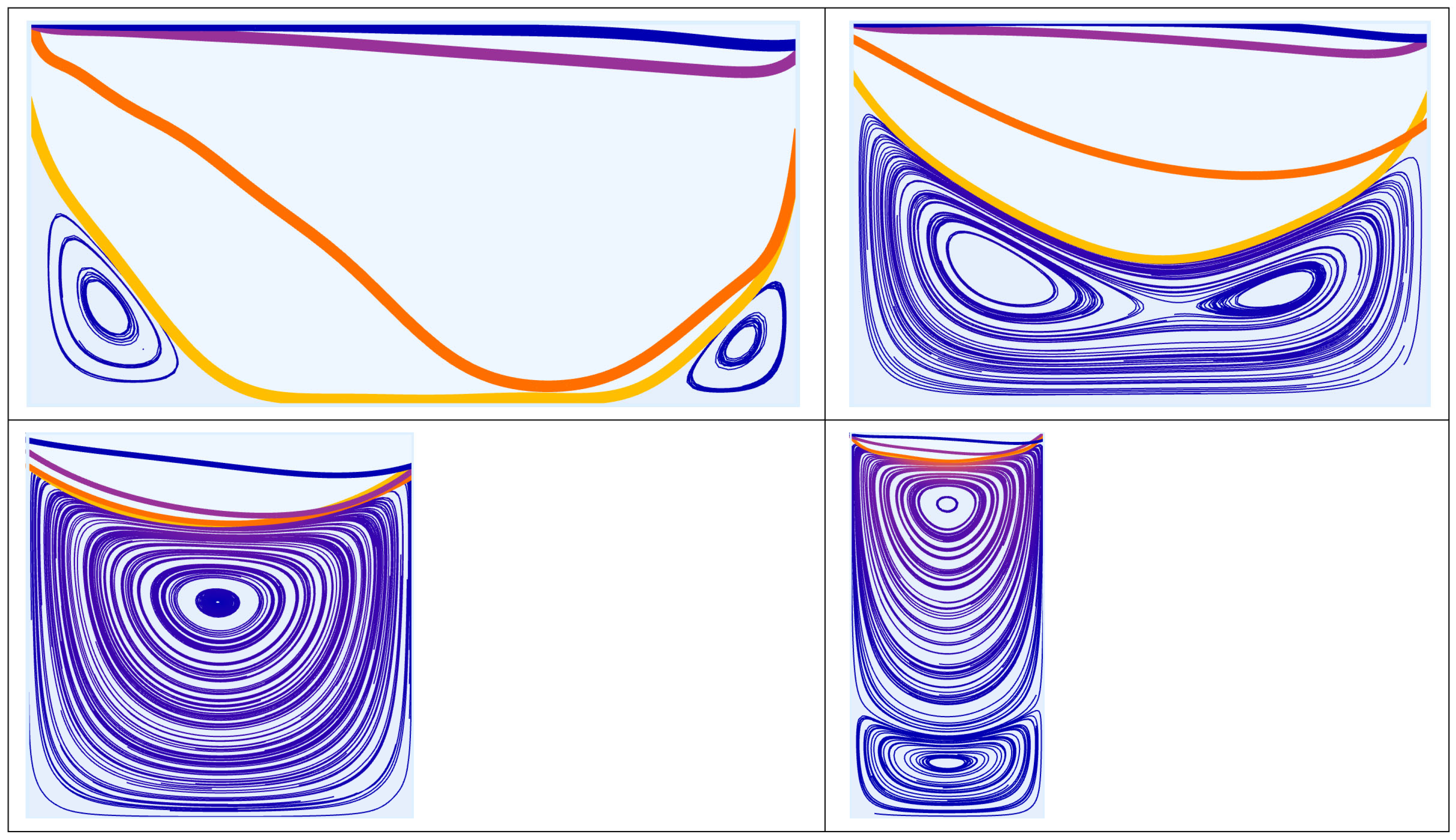
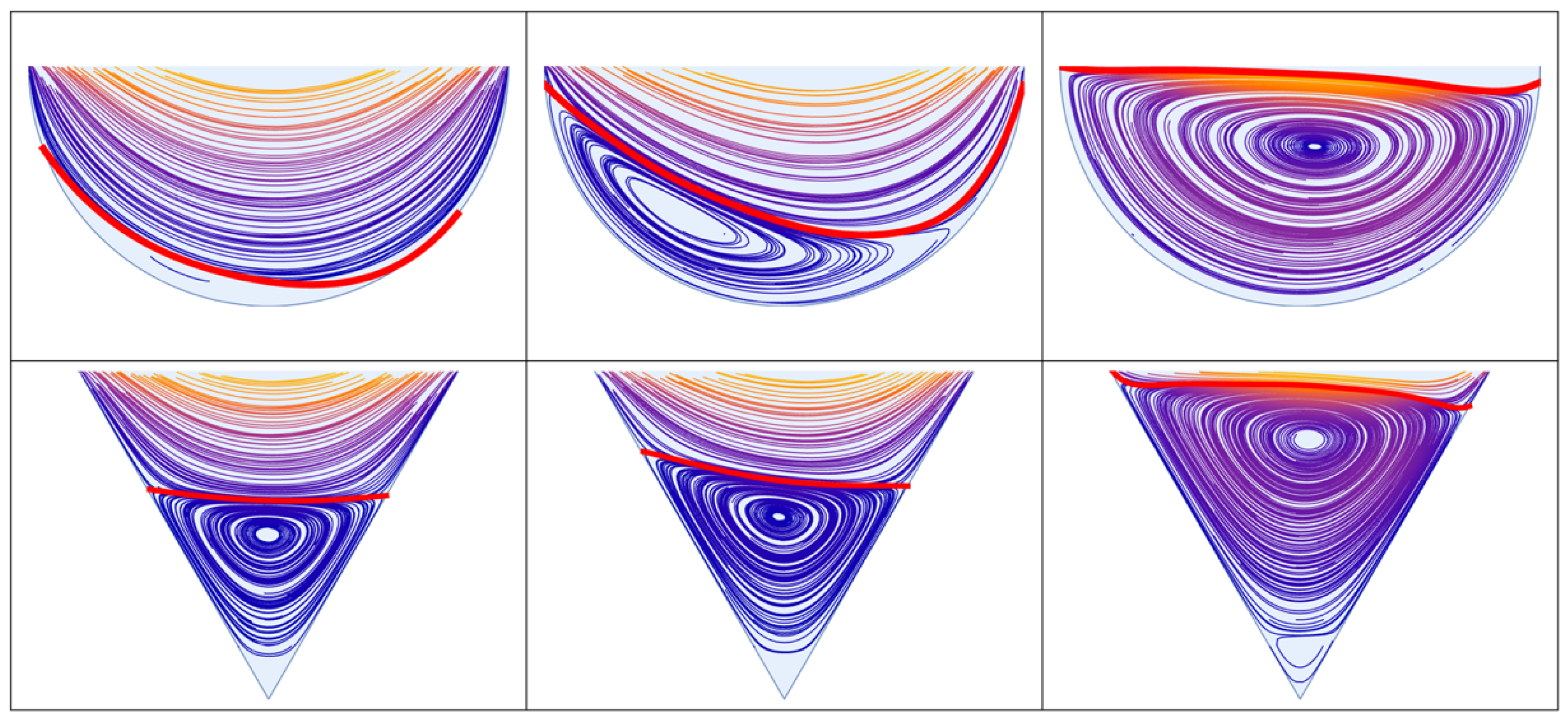
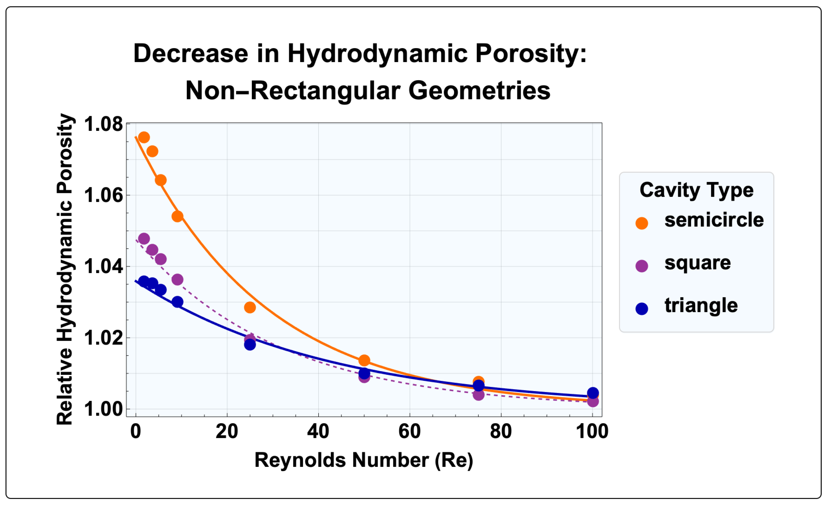
4.2. Separatrix Movement: Non-Rectangular Cavity Geometries

In Figure 11, we provide the stream plots for non-rectangular cavity geometries (i.e., the semicircle and equilateral triangle) with the separatrix highlighted in red.

4.3. Separatrix Movement: Periodic Cavity Geometry

For the reader’s edification, a single stream plot example of the periodic cavity flow geometry is provided below. Additional stream plots are not provided because the streamlines in each cavity are effectively identical for each of the cavity geometries pictured in Figure 12. The purpose of testing periodic flow geometry was to determine the effect of upstream cavities on those downstream. Qualitatively, we can conclude that there is slightly less penetration of the through-flow into the downstream cavity, although this is barely evidenced by the red horizontal line in the figure below. As drawn, this line coincides with the bottom-most point of the separatrix in the upstream cavity. Note that this figure is generated for the periodic flow geometry with cavity spacing one-quarter of the cavity width, at a Reynolds number of 10.

4.4. Applying the Exponential Dependence of Hydrodynamic Porosity on Pore-Scale Flow Velocity

The change in hydrodynamic porosity as a function of the Reynolds number is provided in Figure 13 and Figure 14 below. For ease of comparison across cavity types, we have normalized the hydrodynamic porosity by the value that corresponds to the mobile–immobile zone model. Applied to each dataset, is the exponential dependence of hydrodynamic porosity on pore flow velocity that we previously discovered and described in Equation (1). We remind readers that although it is the value of the pore-space partitioning coefficient that we numerically quantify in this analysis, we are able to plot the hydrodynamic porosity of the medium because of the direct proportionality between these two quantities.

The fitting parameters and coefficient of determination (R²) for each model are summarized in the table below.

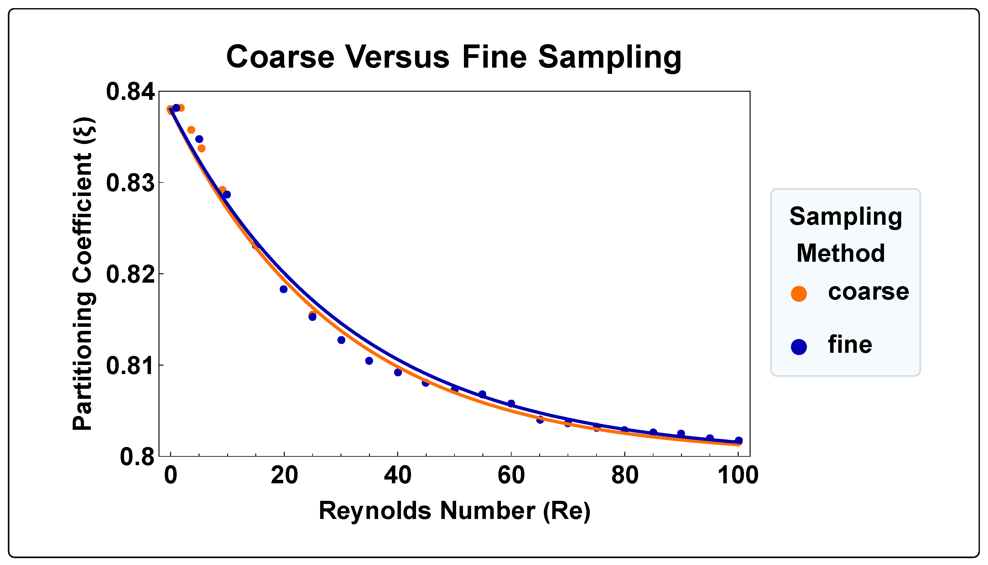
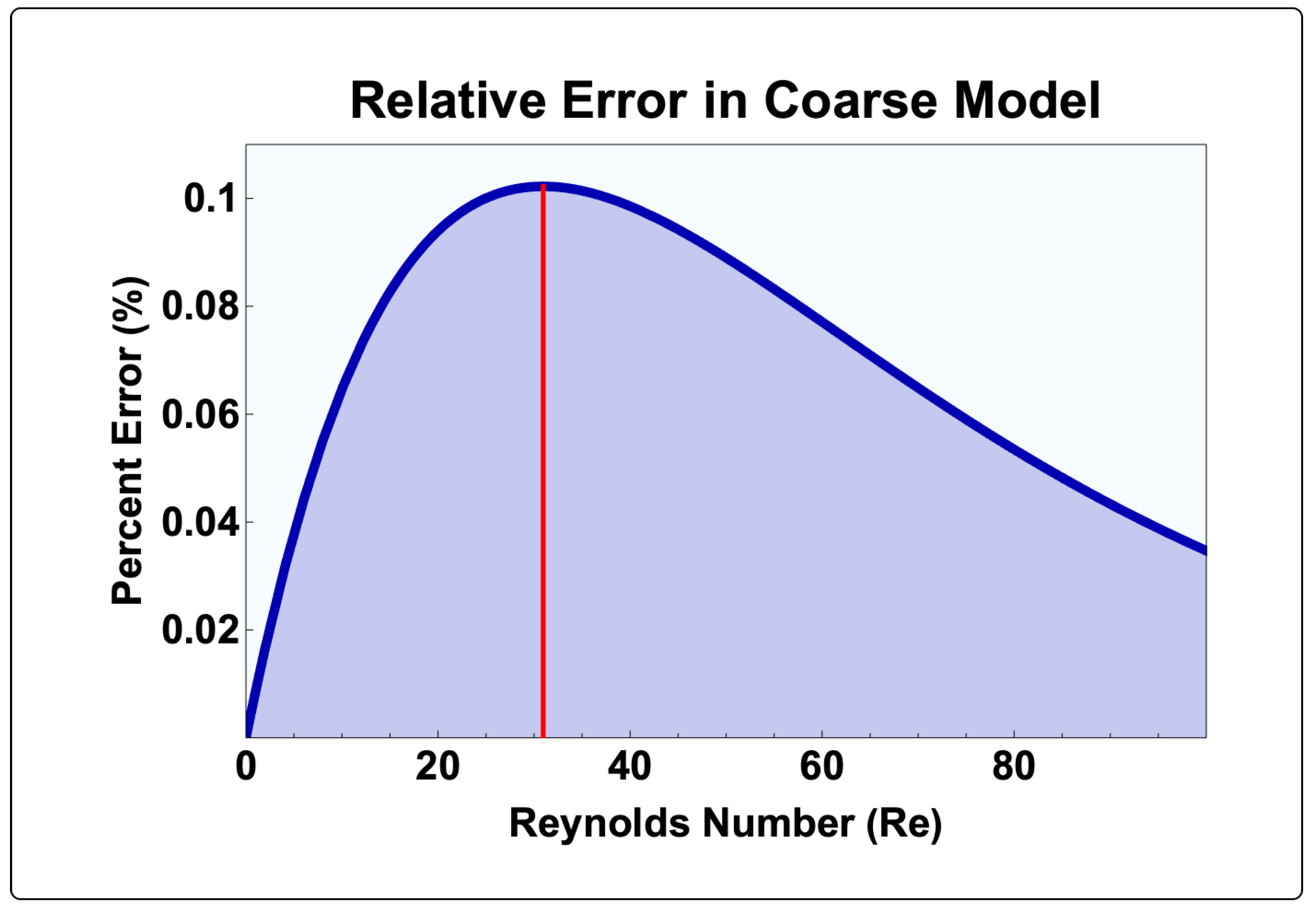
4.5. Sampling Error

Finally, the error associated with the exponential model derived from the relatively sparse dataset is approximated by fitting the exponential model to a more finely sampled dataset pictured in Figure 15 below for the square cavity geometry

5. Discussion

In this work, we find that the pore-space partitioning coefficient ($\xi$) of each of the tested cavity geometries is well-approximated by the exponential relationship in Equation (1). In fact, the coefficient of determination (R²) is approximately one for each dataset. Should we test additional cavity geometries in the future, given representative imaging of the pore space in an unwashed media, it would be reasonable to assume that the partitioning coefficient, and therefore the hydrodynamic porosity of that media, would be well-approximated by this same exponential relationship. Further, our sampling frequency in the previous study did not yield a significant error in our model fit. In fact, when comparing the exponential models that result from both data sets, the largest difference between them is 0.1%. This error is an order of magnitude smaller than the error associated with the measurement process, which we judge to be small enough to disregard in our analysis.

Of the tested geometries, those that exhibited the largest decrease in the pore-space partitioning parameter accompanying an increase in Reynolds number from 1 to 100 were rectangular. More specifically, the two largest decreases were for geometries with a cavity width greater than its depth. When the cavity width was less than its depth, however, the decrease in the pore-space partitioning parameter was the smallest for all the tested geometries. In comparison, adjustment to the cavity depth did not result in such large variations. Although only six rectangular cavities were tested, it appears that the value of the pore-space partitioning parameter is more sensitive to cavity width than cavity depth. Of course, this conclusion is made for a flow geometry with a through-channel height equivalent to either the cavity width or depth. Reduction in the adjacent through-channel height, as we previously demonstrated, results in more significant decreases in the mobile-zone volume. These results are summarized in the table below.

Further increasing the applicability of the exponential dependence of hydrodynamic porosity on pore-scale flow velocity, is the fact that the periodic flow geometries do not exhibit a significant difference between the upstream and downstream cavities. Given this finding, we can more confidently apply our hydrodynamic description of porosity onto a periodic medium at the macroscale.

As previously mentioned, the next steps for this work are in the experimental quantification of the exponential fit parameters in Equation (1) (i.e., a, b, and c). The ability to do so for media at sites needing remediation is necessary to demonstrate the ease with which this relationship can be tailored to a specific media. Further, it may be the case that the numerically calculated parameters provided in

Table 2. Exponential model fit parameters for each cavity geometry. Rectangular cavity geometries are specified by depth-to-width ratio.

	Equation (1) Exponential Fit Parameters
Cavity Geometry	$\mathit{a}$	$\mathit{b}\times {10}^2$	$\mathit{c}\times {10}^2$	${\mathit{R}}^2$
Square	0.80	3.80	3.19	0.9999
Rectangle
2:1	0.67	3.13	3.16	0.9998
1.5:1	0.73	3.41	3.11	0.9999
0.5:1	0.89	6.19	3.26	0.9999
1:2	0.80	16.88	4.26	0.9999
1:1.5	0.80	9.50	4.73	0.9999
1:0.5	0.80	1.14	0.91	0.9999
Circle	0.91	6.94	3.47	0.9999
Triangle	0.90	3.24	2.33	0.9999

and

Table 3. The decrease in pore-space partitioning coefficient ($\xi$) corresponding to an increase in channel-based Reynolds number, from 1 to 100. Rectangular cavity geometries are specified by their cavity depth-to-width ratio.

% Decrease in Pore-Space Partitioning Coefficient, $(\mathit{\xi }={\mathit{\theta }}_{\mathit{m}\mathit{o}\mathit{b}\mathit{i}\mathit{l}\mathit{e}}/\mathit{\theta })$
Cavity Geometry	Dead-End Pore Geometry
Square	4.10
Rectangle
2:1	4.05
1.5:1	4.04
0.5:1	5.91
1:2	16.09
1:1.5	9.73
1:0.5	0.81
Circle	6.45
Triangle	2.99

indicate a physical characteristic of the aggregate, effective pore geometry of real media. For example, consider the rectangular cavities with a depth-to-width ratio of 1:2 and 1:0.5. The former has a b value one order of magnitude larger than the rest, and the latter, a c value one order of magnitude smaller than the rest. The values in Table 2 also serve as an order of magnitude guide for what the exponential fit parameters should be in column studies.

6. Study Limitations

Our algorithm for determining the separatrix location is robust and is presented in our highly legible code available in the Supplementary Materials. Its errors are smaller than the numerical errors of solving the PDEs.

We considered only the immobile zones generated by dead-end pores and cavity-like structures that generate flow separation with the Reynolds number of the interstitial flow of up to about 100.

Our results are derived for Newtonian, incompressible fluids and thus do not apply to non-Newtonian, rheological flows.

Finally, this work focuses on groundwater flow, i.e., single-phase flow through fully saturated porous media with dead-end pores (unwashed sand and gravel, fractured rock, etc.) with pore sizes larger than 2 μm. Consequently, our results do not apply to multiphase flow such as water and air in unsaturated (vadose) zones. And our results do not reflect or account for the phenomena occurring in nanoscale (>1 nm) pores near walls, such as apparent viscosity increases and bound water forming.

7. Conclusions

In this work, we have further demonstrated the applicability of the exponential dependence of hydrodynamic porosity on pore-scale flow velocity. We have done so by testing a range of cavity geometries that are more representative of what we would expect to see in a real porous medium (i.e., rectangular, non-rectangular, and periodic geometries). Previously, we only tested a single, square cavity geometry, which is a highly idealized case. We have shown that not only does this exponential relationship hold for media with these new cavity geometries, but it does so almost perfectly with a coefficient of determination (R²) of approximately one for each set of simulation data. Given this high fit quality, it is evident that the exponential relationship we previously discovered is applicable to most, if not all, media with dead-ended pore spaces. That said, this work would lend itself well to significant expansion. Although we have highlighted sensitivity to cavity width, and previously, through-channel height to pore depth, there remain other parameters that could affect the exponential fit and perhaps, even inform us about the aggregate, effective nature of the pore spaces of experimentally studied media.

References

- Worthington, S.R. Estimating effective porosity in bedrock aquifers. Groundwater 2022, 60, 169–179. [Google Scholar] [CrossRef]
- Yan, S.; Yang, M.; Sun, C.; Xu, S. Liquid Water Characteristics in the Compressed Gradient Porosity Gas Diffusion Layer of Proton Exchange Membrane Fuel Cells Using the Lattice Boltzmann Method. Energies 2023, 16, 6010. [Google Scholar] [CrossRef]
- Meier, H.; Zimmerhackl, E.; Zeitler, G. Modeling of colloid-associated radionuclide transport in porous groundwater aquifers at the Gorleben site, Germany. Geochem. J. 2003, 37, 325–350. [Google Scholar] [CrossRef]
- Coats, K.H.; Smith, B.D. Dead-End Pore Volume and Dispersion in Porous Media. Soc. Petrol. Eng. J. 1964, 4, 73–84. [Google Scholar] [CrossRef]
- Yuan, Y.; Rezaee, R. Comparative Porosity and Pore Structure Assessment in Shales: Measurement Techniques, Influencing Factors and Implications for Reservoir Characterization. Energies 2019, 12, 2094. [Google Scholar] [CrossRef]
- Li, B.; Li, X.-S.; Li, G.; Jia, J.-L.; Feng, J.-C. Measurements of Water Permeability in Unconsolidated Porous Media with Methane Hydrate Formation. Energies 2013, 6, 3622–3636. [Google Scholar] [CrossRef]
- Foroughi, S.; Bijeljic, B.; Gao, Y.; Blunt, M.J. Incorporation of Sub-Resolution Porosity into Two-Phase Flow Models with a Multiscale Pore Network for Complex Microporous Rocks. Water Resour. Res. 2024, 60, e2023WR036393. [Google Scholar] [CrossRef]
- Verbovšek, T. Variability of Double-Porosity Flow, Interporosity Flow Coefficient λ and Storage Ratio ω in Dolomites. Water 2024, 16, 1072. [Google Scholar] [CrossRef]
- Fenni, M.; Guellal, M.; Hamimid, S. Influence of Porosity Properties on Natural Convection Heat Transfer in Porous Square Cavity. Phys. Fluids 2024, 36, 056108. [Google Scholar] [CrossRef]
- Kango, R.; Chandel, A.; Shankar, V. A Statistical Model for Estimating Porosity Based on Various Parameters of Flow Through Porous Media. Water Pract. Technol. 2024, 19, 1936–1947. [Google Scholar] [CrossRef]
- Yao, P.; Zhang, J.; Qin, Z.; Fan, A.; Feng, G.; Vandeginste, V.; Zhang, P.; Zhang, X. Effect of Pore Structure Heterogeneity of Sandstone Reservoirs on Porosity-Permeability Variation by Using Single-Multi-Fractal Models. ACS Omega 2024, 9, 23339–23354. [Google Scholar] [CrossRef] [PubMed]
- Young, A.H.; Kabala, Z.J. Hydrodynamic Porosity: A New Perspective on Flow Through Porous Media, Part I. Water 2024, 16, 2158. [Google Scholar] [CrossRef]
- van Genuchten, M.T.; Wierenga, P.J. Mass-Transfer Studies in Sorbing Porous-Media. I. Analytical Solutions. Soil Sci. Soc. Am. J. 1976, 40, 473–480. [Google Scholar] [CrossRef]
- Moffatt, H.K. Viscous and Resistive Eddies near a Sharp Corner. J. Fluid Mech. 1963, 18, 1–18. [Google Scholar] [CrossRef]
- Higdon, J.J.L. Stokes Flow in Arbitrary Two-Dimensional Domains: Shear Flow over Ridges and Cavities. J. Fluid Mech. 1985, 159, 195–226. [Google Scholar] [CrossRef]
- Shen, C.; Floryan, J.M. Low Reynolds Number Flow over Cavities. Phys. Fluids 1985, 28, 3191–3202. [Google Scholar] [CrossRef]
- Fang, L.C.; Cleaver, J.W.; Nicolaou, D. Hydrodynamic Cleansing of Cavities. In Proceedings of the 8th International Conference on Computational Methods and Experimental Measurements (CMEM 97), Rhodes, Greece, 21–23 May 1997; pp. 391–401. [Google Scholar]
- Mehta, U.B.; Lavan, Z. Flow in a Two-Dimensional Channel with a Rectangular Cavity. J. Appl. Mech. 1969, 36, 897–901. [Google Scholar] [CrossRef]
- O’Brien, V. Closed Streamlines Associated with Channel Flow over a Cavity. Phys. Fluids 1972, 15, 2089–2097. [Google Scholar] [CrossRef]
- O’Neill, M.E. Separation of a Slow Linear Shear-Flow from a Cylindrical Ridge or Trough in a Plane. Z. Angew. Math. Phys. 1977, 28, 439–448. [Google Scholar] [CrossRef]
- Kahler, D.M.; Kabala, Z.J. Acceleration of Groundwater Remediation by Deep Sweeps and Vortex Ejections Induced by Rapidly Pulsed Pumping. Water Resour. Res. 2016, 52, 3930–3940. [Google Scholar] [CrossRef]
- Kang, I.S.; Chang, H.N. The Effect of Turbulence Promoters on Mass-Transfer—Numerical-Analysis and Flow Visualization. Int. J. Heat Mass Transf. 1982, 25, 1167–1181. [Google Scholar] [CrossRef]
- Alkire, R.C.; Deligianni, H.; Ju, J.B. Effect of Fluid-Flow on Convective-Transport in Small Cavities. J. Electrochem. Soc. 1990, 137, 818–824. [Google Scholar] [CrossRef]
- Horner, M.; Metcalfe, G.U.; Wiggins, S.; Ottino, J.M. Transport Enhancement Mechanisms in Open Cavities. J. Fluid Mech. 2002, 452, 199–229. [Google Scholar] [CrossRef]
- Wolfram Numerical Solutions of PDEs. Available online: https://reference.wolfram.com/language/tutorial/NDSolvePDE.html (accessed on 15 June 2024).
- Takematsu, M. Slow viscous flow past a cavity. J. Phys. Soc. Jpn. 1966, 21, 1816–1821. [Google Scholar] [CrossRef]
- Friedman, M. Flow in a circular pipe with recessed walls. J. Fluid Mech. 1970, 37, 5–8. [Google Scholar] [CrossRef]
- Stevenson, J.F. Flow in a tube with a circumferential wall cavity. J. Appl. Mech. Trans. ASME 1973, 40, 355–361. [Google Scholar] [CrossRef]
- Driesen, C.H.; Kuerten, J.G.M.; Streng, M. Low-Reynolds-number flow over partially covered cavities. J. Eng. Math. 1998, 34, 3–21. [Google Scholar] [CrossRef]
- Taneda, S. Visualization of separating Stokes flows. J. Phys. Soc. Jpn. 1979, 46, 1935–1942. [Google Scholar] [CrossRef]
- Shankar, P.N.; Deshpande, M.D. Fluid Mechanics in the Driven Cavity. Annu. Rev. Fluid Mech. 2000, 32, 93–136. [Google Scholar] [CrossRef]
- Laskowska, A. Experimental Studies of Flows in Porous Media and Selected Models of the Pore Space. Ph.D. Dissertation, Strata Mechanics Research Institute Polish Academy, Krakow, Poland, 1996; p. 179. [Google Scholar]
- Pan, F.; Acrivos, A. Steady flows in rectangular cavities. J. Fluid Mech. 1967, 28, 643–655. [Google Scholar] [CrossRef]
- Jolls, K.R.; Hanratty, T.J. Transition to Turbulence for Flow through a Dumped Bed of Spheres. Chem. Eng. Sci. 1966, 21, 1185–1191. [Google Scholar] [CrossRef]
- Wegner, T.H.; Karabelas, A.J.; Hanratty, T.J. Visual Studies of Flow in a Regular Array of Spheres. Chem. Eng. Sci. 1971, 26, 59–63. [Google Scholar] [CrossRef]
- Latifi, M.A.; Midoux, N.; Storck, A.; Gence, J.N. The Use of Micro-Electrodes in the Study of the Flow Regimes in a Packed-Bed Reactor with Single-Phase Liquid Flow. Chem. Eng. Sci. 1989, 44, 2501–2508. [Google Scholar] [CrossRef]
- Rode, S.; Midoux, N.; Latifi, M.A.; Storck, A.; Saatdjian, E. Hydrodynamics of Liquid Flow in Packed Beds: An Experimental Study Using Electrochemical Shear Rate Sensors. Chem. Eng. Sci. 1994, 49, 889–900. [Google Scholar] [CrossRef]
- Bu, S.; Yang, Y.; Zhang, X.; Tao, W. Experimental Study of Transition Flow in Packed Beds of Spheres with Different Particle Sizes Based on Electrochemical Microelectrodes Measurement. Appl. Therm. Eng. 2014, 73, 1525–1532. [Google Scholar] [CrossRef]
- Elderkin, R.H. Separatrix Structure for Elliptic Flows. Am. J. Math. 1975, 97, 221–247. [Google Scholar] [CrossRef]
- Weiss, J.B. Transport and Mixing in Traveling Waves. Phys. Fluids A 1991, 3, 1379–1384. [Google Scholar] [CrossRef]