Water Quality in Estero Salado of Guayaquil Using Three-Way Multivariate Methods of the STATIS Family

Abstract

Water property parameters were analyzed over 9 months across six stations within the Estero Salado. The parameters under evaluation included nitrite (NO₂⁻), nitrate (NO₃⁻), phosphate (PO₄³⁻), ammonium (NH₄⁺), temperature, pH, biochemical oxygen demand (BOD), conductivity, salinity, color, turbidity, suspended solids, hardness, and alkalinity. Additionally, the TRIX index (which measures chlorophyll, oxygen saturation, nitrogen, and phosphorus) was considered. The multivariate technique employed was partial triadic analysis (PTA), a specialized variant developed from STATIS, enabling the examination of the common structure’s stability across months and the positioning of stations and variables within a compromise space. This analysis elucidated a variability of 69% and 96%, respectively. Stations could be characterized based on their associations with specific variables, while the analysis also facilitated the identification of months impacting the common structure of pollution indicators.

1. Introduction

An extensive arm of the sea, with a length of more than 50 km, approaches the city from the south, showing a series of branches along its route, among which stand out the Estero Cobina, the Estero del Muerto, the Estero Santa Ana, and the Estero Salado, located in the vicinity of Guayaquil. These estuaries experience constant ebbs and flows of ocean tides, creating a diverse ecosystem rich in fauna and flora, characterized especially by the predominant presence of mangroves on their margins [1].

Freshwater ecosystems, particularly streams and rivers, are among the most critically endangered ecosystems globally. This endangerment is attributed to the combined effects of natural variability, including geological, hydrological, and climatic factors, as well as heightened anthropogenic activities such as rapid industrialization and agriculture, which result in the extensive use of chemical fertilizers and pesticides [2]. During the decades of the 50s and 60s, Guayaquil experienced uncontrolled urban growth, where mangrove areas in the Estero Salado were occupied for the construction of homes and industries without adequate territorial planning. This lack of regulation led to the direct discharge of domestic and industrial waste into the Estero Salado, generating significant environmental impacts and affecting the biodiversity of the area [3].

The Estero Salado is the largest and one of the most productive in the city, concentrating approximately 81% of Ecuador’s mangrove system [4]. However, in the city, 70% of the registered industries are located in the area near the estuaries. Of these, the food product industry represents 70% of the total number of industrial plants. An annual discharge of 6,000,000 cubic meters of oil and grease is estimated, especially in Guayaquil, and the metal–mechanical industry contributes a discharge of 16,000,000 cubic meters per year [5]. The Technical Standard for the Control of Liquid Discharges evidences the alterations in water quality and the presence of eutrophication in the estuarine zone of the Estero Salado. The Ecuadorian state has recognized the seriousness of this situation through an inventory of polluting companies within the framework of the Ecological Guayaquil Project [6]. Therefore, it is important to evaluate water quality and review eutrophication processes in the estuarine zone.

To evaluate the water quality in the Estero Salado, measurements were carried out at seven sampling stations strategically located along the estuary. At these stations, various chemical concentrations and physicochemical parameters were determined, including levels of nitrite (NO₂⁻), nitrate (NO₃⁻), phosphate (PO₄³⁻), and ammonium, as well as measurements of temperature, pH, and biochemical oxygen demand (BOD). The indices of electric conductivity, salinity, color, turbidity, suspended solids, hardness, and alkalinity were also evaluated, thus providing a complete overview of the environmental quality of the estuarine ecosystem in question. TRIX, which is based on measurements of chlorophyll, oxygen saturation, nitrogen and phosphorus, was used as an indicator of trophic status at a given time. This index is crucial to classify the trophic state of coastal water bodies such as the Estero Salado, dividing them into categories ranging from oligotrophic to hypereutrophic [7].

To properly analyze the data, three-way table analysis methods were employed, which hold significant importance in multivariate statistical analysis. This type of table includes a first entry that identifies the individuals who are the object of study, a second entry for the variables that have been measured for those individuals, and a third entry for the various situations (time, location, or conditions) in which measurements are made. Standard multivariate statistical techniques, such as principal component analysis and hierarchical cluster analysis, have been widely used as unbiased methods for extracting meaningful information from groundwater quality data [8]. However, these classical multivariate methods typically handle two-way matrices (individuals × variables or individuals × time), whereas datasets resulting from qualitative water monitoring programs often need to be conceptualized as a data cube (individuals × variables × time).

Partial triadic analysis (PTA) has been extensively utilized in numerous studies across a range of disciplines. In the ecological domain, PTA has proven invaluable for analyzing complex interactions within ecosystems and understanding biodiversity patterns [9,10,11,12]. Its application in education has facilitated the assessment of education policies [13]. Within the sphere of water quality, PTA has been instrumental in identifying and evaluating the factors affecting aquatic environments, thereby aiding in the development of effective management and conservation plans [14,15]. Moreover, in the social domain, PTA has been applied to analyze the impact of significant events such as crime [16], economics [17], and COVID-19, providing a nuanced understanding of their effects on public health and society [18,19]. This versatile analytical method continues to be a powerful tool for researchers seeking to uncover intricate relationships within diverse datasets.

There are three studies that have used PTA to analyze water quality. The first analyzed the spatial and temporal patterns of water quality in a river in northeastern Spain [20], the second examined pollution in agricultural landscapes of a river in northeastern Spain [21], and the third determined the degree of water pollution in both anthropogenic and natural settings in North Africa [22].

The primary objective was to identify the water quality using all the properties of water for the calculation of the Trophic State Index (TRIX) for the six stations of the Estero Salado of Guayaquil over 9 months, using a three-way multivariate technique: partial triadic analysis (PTA) of the STATIS family.

2. Materials and Methods

2.1. Experimental Design

Several coastal areas such as Guayas are characterized by an arid tropical climate, with a wet season of high temperatures and abundant rainfall extending from December to April or May, influenced by the presence of the warm El Niño current and the Intertropical Convergence Zone. On the other hand, the dry season is marked by low temperatures and scant precipitation, spanning from June to November or December. Specifically, Guayaquil is situated at an average altitude of 20 m above sea level, with an average temperature ranging between 26 °C and 27 °C and an annual relative humidity of 85% [23].

During 2022, seven water samples were randomly collected (water aliquots) at seven stations (bridges) located in the city of Guayaquil, Guayas, Ecuador, as shown in Figure 1. One sample was collected at each station during the first week of nine months from March to December, excluding July. These stations were selected due to their location in areas of high population density and significant anthropogenic activity within the city and its surroundings [4]. The sample selection criteria adhered to the NTE INEN 2176 standard [24], and were based on ease of access, safety, and uniformity in depth, avoiding dammed and turbulent areas that were not representative.

The samples were classified, refrigerated if necessary, and duly transferred to the laboratory to guarantee their usefulness.

2.2. Analytical Procedure

The parameters or indicators analyzed in this study are presented in

Table 1. Information on variables considered.

Parameter	Indicator	Unit of Measurement
Inorganic nutrients	Nitrite (NO2−)	mg/L
	Nitrate (NO3−)	mg/L
	Ammonium (NH4+)	mg/L
	Ortho-phosphate (PO43−)	mg/L
Chemical indicators	Dissolved oxygen (DO)	mg/L
	pH	U-pH
	Biochemical oxygen demand (BOD)	mg/L
	Total alkalinity (TA)	mg/L
	Total hardness (TH)	mg/L
	Salinity (SI)	mg/L
Physical indicators	Turbidity (TT)	NTU
	Color (C)	mg/L
	Suspended solids (SSs)	mg/L
	Temperature (T)	°C
	Electric conductivity (EC)	NTU
Contamination indicator	Trophic index (TRIX)	-

.

Throughout the study, a total of 63 samples were collected. Physicochemical parameters such as turbidity, color, suspended solids, electrical conductivity, pH, and temperature were analyzed in situ using a portable Hach multimeter (model HQ40D) and a turbidimeter (model 2100Q). These characteristics of the water were measured using the established Standard Methods for the Examination of Water and Wastewaters [25].

For the determination of inorganic compounds such as nitrites and nitrates, a Hach spectrophotometer, model DR3900, was used. Other chemical indicators, including dissolved oxygen (DO), biochemical oxygen demand (BOD), total alkalinity (TA), total hardness (TH), and salinity (SI), were analyzed using test kits, an automatic titrator, and clean sterile containers, respectively. To ensure the representativeness of the samples, they were refrigerated, labeled, and transported in sealed ice containers to the microbiology laboratory of Ecuahidrolizados SAS to prevent contamination and changes in composition. The samples were stored between 2 °C and 5 °C in a refrigerator until analysis in the following hours to preserve their chemical integrity, in accordance with the NTE INEN 2169:2013 standard [26].

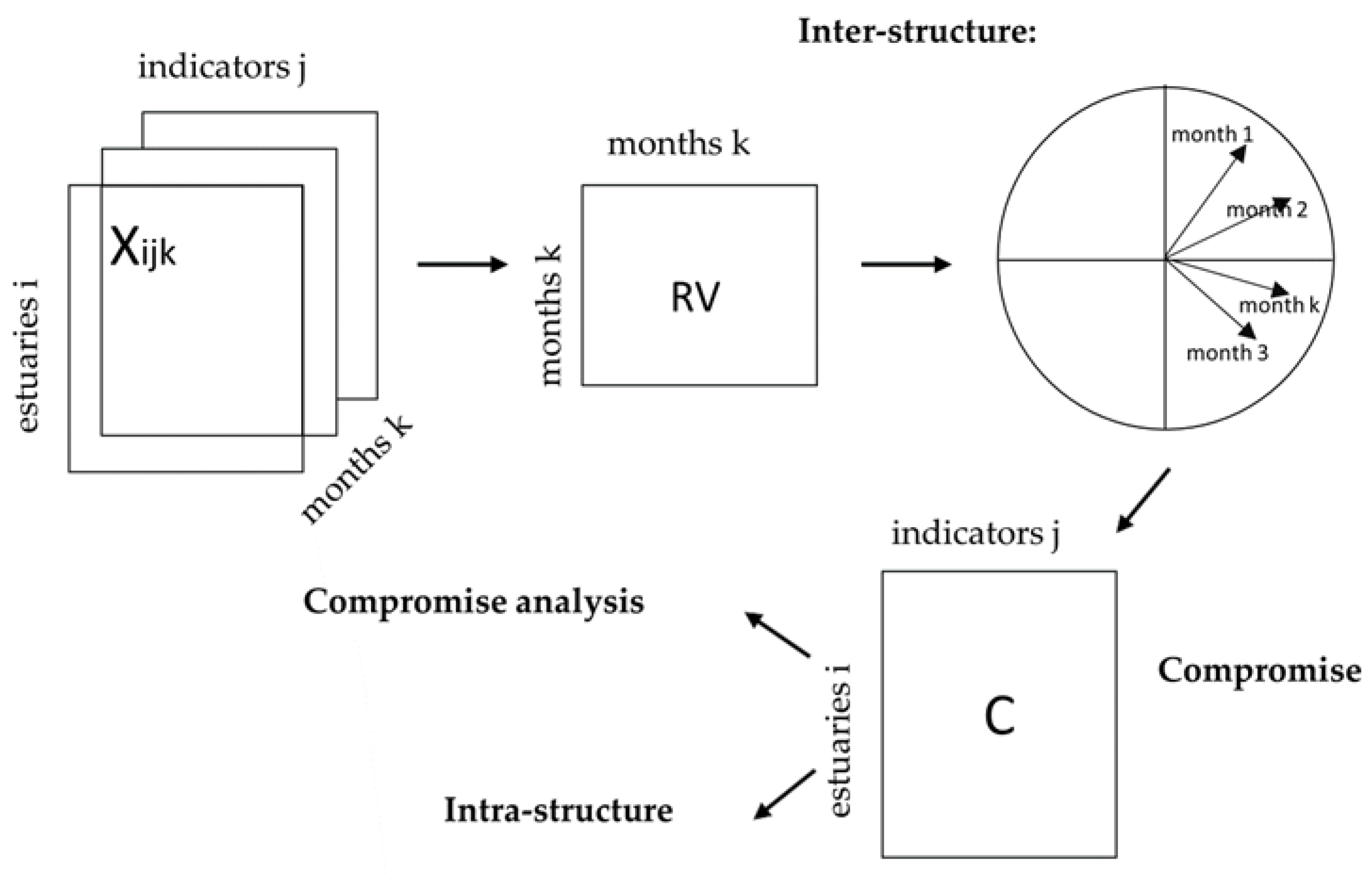
2.3. Partial Triadic Analysis

The data used in analysis consists of K = 9 tables and constitutes the so-called data cube: objects (n = 7 stations) variables (p = 16 indicators) time (9 months). In this article, the primary objective is to analyze the differences and similarities between the different scenarios through the configurations of individuals and relationships between different groups of variables.

The analytical approach employed in this article to scrutinize the three-way data structure was partial triadic analysis (PTA), a method affiliated with the STATIS methodology. The name STATIS is an acronym for the French expression ‘Structuration des tableaux à trois indices de la statistique’, which can roughly be translated as “structuring three-way statistical tables” [27]. STATIS employs as its principal analytical tool the singular value decomposition (SVD) and the generalized singular value decomposition (GSVD) of a matrix. This tool is applied in a second step, utilizing the set of optimal weights resulting from the inter-structure analysis, with which it performs a generalized PCA of an object X (intra-structure). Due to this similarity in analysis, STATIS is considered part of the PCA family [28].

On the other side, partial triadic analysis (PTA), also called X-STATIS [29], is an analytical technique for three-dimensional data that works directly with the original matrices without using operators. Unlike other methods in the STATIS family, it is more restrictive in that it assumes that the same variables are measured in the same individuals. However, it does not lose original information, allowing for more representations. This method is useful for analyzing three-dimensional data, as it provides a clear visual representation of the relationships between different datasets and allows an overall graphical comparison of the tables by projecting them onto the principal component analysis (PCA) factor map [30]. Therefore, when applied to the physicochemical parameters of water measured in different locations and times, it helps identify patterns and trends, with the aim of understanding how these characteristics may be interrelated or how they vary from one place to another and over time.

PTA encompasses three primary objectives: firstly, to analyze the similarity structure of the set of tables (inter-structure); secondly, to integrate these datasets into an optimal weighted average (compromise), which is subsequently subjected to principal component analysis (PCA) to unveil the shared structure among the observations; and lastly, to project each of the original datasets onto the compromise to scrutinize commonalities and discrepancies (intra-structure) [27]. Below, a brief description of each step is provided.

2.3.1. Step 1: Inter-Structure

Let X₁, … X_K … X_K be the K tables of quantitative variables with the same n rows (objects) and the same p columns (variables). Let (X₁, Q, D) … (X_k, Q, D) … (X_k, Q, D) be the associated statistical triplets [16], where:

• Q_k(p×p): Weight symmetric matrix for the table variables X_k(n×p) and is a metric used as an inner product in Rp allowing to measure distances between the n objects. When the variables are centered and reduced, then matrix Q_k is the identity matrix.
• D_n×n: Weight matrix corresponding to the stations, defined as a diagonal matrix where each element represents the weight assigned to an individual. This configuration allows D_n×n to be used as a metric in Rⁿ space, providing a means to assess interactions among the p variables. For this specific study, the weights for all stations are standardized, assigning a uniform value of $\raisebox{1ex}{$1$}\!\left/ \!\raisebox{-1ex}{$\mathrm{n}$}\right.$ to each.

The inter-structure analysis is based on the concepts of vector correlation coefficients between tables, also called RV-coefficients, proposed by Robert and Escoufier (1976) [31]:

$$RV {\mathit{X}}_{\mathit{k}},{\mathit{X}}_{\mathit{l}}={\displaystyle \frac{Covv ({\mathit{X}}_{\mathit{k}},{\mathit{X}}_{\mathit{l}})}{\sqrt{Vav\left({\mathit{X}}^k\right)}\sqrt{Vav\left({\mathit{X}}^l\right)}}}$$

where $Covv \left({\mathit{X}}_{\mathit{k}},{\mathit{X}}_{\mathit{l}}\right)=tr\left({\mathbf{X}}_k^T\mathit{D}{\mathit{X}}_{\mathit{K}}\mathit{Q}\right).$ The matrix with all the RV coefficients is defined as:

$${\mathit{R}\mathit{V}}_{\left(\mathit{k}\times \mathit{k}\right)}={ [RV{(\mathit{X}}_{\mathit{k}},{\mathit{X}}_{\mathit{l}})]}_{i,j}$$

The calculation of the RV coefficient matrix among stations facilitates the evaluation of station comparability and the depiction of their proximity [14]. The eigenvalues Θ and the normed eigenvectors U of the RV matrix are used to computed the scores of tables (G = UΘ 2), which are presented in Figure 2 through a correlation circle [16].

2.3.2. Step 2: Compromise

The compromise analysis is carried out on the basis of the results obtained in the inter-structure step, where the compromise table can be defined as:

$$X_C=\sum _{\mathrm{k}}^{\mathrm{K}}{\alpha }_k{X}_K$$

where:

• u₁ is the first eigenvector of the matrix U.
• (${\alpha }_1$, …, ${\alpha }_k$) are the components of the eigenvector, where each acts as a weight assigned to the corresponding table X_k.
• ${\sum }_{k=1}^k{\alpha }_k=1$. For k = 1, …, K; this condition specifies that the total sum of the weights ${\alpha }_k$ must be equal to 1.

The analysis of the compromise is explained by the statistical triplet (X_C, Q, D) with the use of PCA, given by:

$$L=X_{C}QA$$

$$C=X_C^{T}DB$$

where:

• L: Row scores, projection of the rows of X_C onto the principal axes A.
• X_C: Matrix used for the projections; involves both rows for L and columns (as $X_C^T$) for C.
• Q: Transformation matrix that, together with A, aligns X_C to the principal axes.
• A: Principal axes onto which the rows of X_C are projected.
• C: Column scores, projection of the columns of X_C (via $X_C^T$) onto the principal components B.
• D: Weighting matrix that, together with B, aligns the transposed X_C to the principal components.
• B: Principal components onto which the columns of X_C are projected.

2.3.3. Step 3: Intra-Structure

Let Δ be the eigenvalues and A the eigenvectors from the compromise analysis, indicating the amount of variance each principal axis explains. The rows of each initial table are projected onto the principal axes, and columns of each initial table are projected onto the principal components respectively given by:

$$R_k=X_{k}QA$$

$$C_k=X_C^{T}DB$$

where:

• R_K: Row scores for table k, calculated by projecting X_k onto the principal axes A using transformation matrix Q.
• C_K: Column scores for table k, derived from projecting the transposed columns of X_k (denoted $X_C^T$) onto the principal components B with weighting matrix D.

All operations, including the two-dimensional representations, extraction of components, and coordinates of the stations, months, and chemical characteristics, were conducted using the “ade4” package in the R working environment, version 4.1 (2024) [32].

3. Results and Discussion

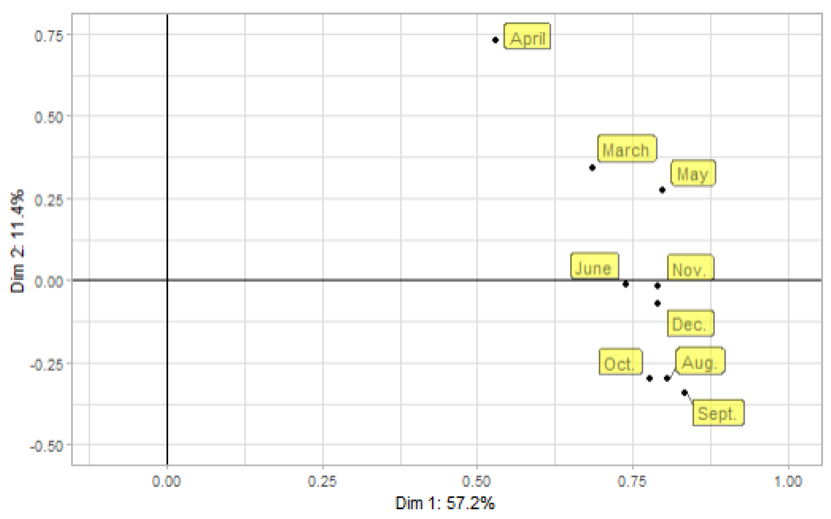
3.1. Inter-Structure Analysis

This decomposition of singular values and successive analysis of principal components reveals a two-dimensional space that captures 69% of the information contained in the RV matrix, mostly retained in the first dimension (

Table A1. Inter-structure summary.

	Dim 1	Dim 2
Eigenvalues	5.152	1.0
Inertia	0.572	0.114
Accumulated inertia	0.572	0.686

).

Except for April, the coordinates of the factorial structure of all months (values greater than 0.6) are mostly associated with the first dimension, presented in

Table A2. Coordinates of the Euclidean image of the inter-structure.

	Dim 1	Dim 2
March	0.687	0.341
April	0.531	0.730
May	0.800	0.275
June	0.740	−0.013
August	0.808	−0.301
September	0.835	−0.340
October	0.778	−0.301
November	0.792	−0.018
December	0.792	−0.072

.

Figure 3 allows us to visualize high stability in the data structure for May, August, September, October, November, and December, proven by the presentation of similar norms and high RV coefficients, as well as confirmed by the coefficients of the first eigenvector (

Table A3. Weights of the first eigenvector.

Month	α
March	0.303
April	0.234
May	0.352
June	0.326
August	0.356
September	0.368
October	0.343
November	0.349
December	0.349

). It illustrates the relationships among different months based on the two principal components derived from PTA. The points representing the different months are clustered, indicating similarities. April is distinctly positioned in the upper left, separate from the other months, suggesting that it possesses unique characteristics not shared with other months. This could be due to the specific climatic conditions in April, such as the end of the rainy season, which significantly impacts the esteros in Guayaquil, Ecuador. Conversely, March and May are closely positioned, indicating that they have similar characteristics, likely influenced by the transition between the rainy and dry seasons, affecting water levels and biodiversity in the estuaries.

Furthermore, June, November, and December are grouped together, as are October, August, and September. This grouping indicates a high degree of similarity among these months, possibly due to consistent climatic patterns and human activities such as urbanization that affect water quality and ecosystem health in the estuaries. In addition, the distance between the points reflects the degree of similarity or dissimilarity: closer points (e.g., March and May) indicate higher similarity, whereas more distant points (e.g., April and December) suggest greater differences, likely caused by seasonal variations and their subsequent impact on estuary environments.

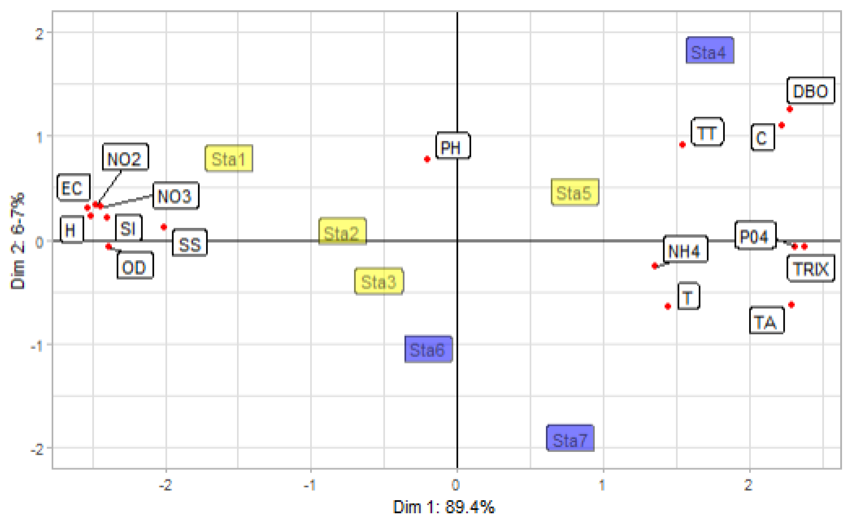
3.2. Compromise Analysis

With the application of singular value decomposition and subsequent principal component analysis, a factorial space is detected that captures in two dimensions 96.2% of the total inertia, with 89.4% and 6.7% retained by the first and second dimensions, respectively (

Table A4. Compromise summary.

	Dim 1	Dim 2
Eigenvalues	73.013	5.492
Inertia	0.894	0.067
Accumulated inertia	0.894	0.962

). The coordinates of the factor structure are presented in

Table A5. Compromise factor coordinates.

	Dim 1	Dim 2
Sta1	−1.343	0.612
Sta2	−1.007	0.261
Sta3	−0.756	−0.213
Sta4	1.510	1.645
Sta5	0.586	0.287
Sta6	0.017	−0.867
Sta7	0.993	−1.724

.

The analysis of the compromise reveals a significant distinction along dimension 1, which primarily discriminates between stations based on the concentrations of inorganic nutrients and contaminants. Figure 4 indicates how stations positioned on the left side of axis 1 (negative dimension 1) are characterized by higher concentrations of inorganic nutrients, specifically nitrite (NO₂⁻) and nitrate (NO₃⁻), with 0.15 mg/L and 0.68 mg/L, respectively. Additionally, these stations exhibit elevated levels of certain physical and chemical indicators, such as electrical conductivity (EC), salinity (SI), suspended solid (SSs), dissolved oxygen (DO), and total hardness (H) (

Table A7. Means ± standard deviation of water indicators by station.

Parameter	Indicator	E1	E2	E3	E4	E5	E6	E7
Inorganic nutrients	NO2− (mg/L)	0.15 ± 0.065	0.13 ± 0.066	0.12 ± 0.055	0.01 ± 0.021	0.04 ± 0.048	0.06 ± 0.049	0.02 ± 0.024
	NO3−(mg/L)	0.68 ± 0.321	0.73 ± 0.401	0.61 ± 0.389	0.1 ± 0.073	0.16 ± 0.233	0.32 ± 0.355	0.1 ± 0.144
	NH4+ (mg/L)	0.17 ± 0.15	0.33 ± 0.234	0.39 ± 0.331	1.12 ± 1.445	0.81 ± 0.853	0.66 ± 0.698	1.05 ± 1.089
	PO43− (mg/L)	0.55 ± 0.278	0.73 ± 0.416	0.98 ± 0.596	1.89 ± 1.351	1.39 ± 1.005	1.18 ± 0.732	1.68 ± 1.161
Chemical indicators	DO (mg/L)	2.89 ± 0.625	2.69 ± 0.458	2.29 ± 0.768	0.49 ± 0.481	0.94 ± 0.78	2.15 ± 1.112	0.79 ± 0.631
	pH (U-pH)	7.58 ± 0.319	7.56 ± 0.196	7.52 ± 0.195	7.59 ± 0.243	7.48 ± 0.194	7.51 ± 0.237	7.5 ± 0.246
	BOD (mg/L)	6.8 ± 3.529	6.58 ± 3.248	6.27 ± 3.217	26.05 ± 7.824	18.67 ± 7.495	10.6 ± 2.645	11.53 ± 4.327
	TA (mg/L)	129.71 ± 5.844	132.44 ± 7.355	140.03 ± 8.256	164.38 ± 21.713	150.48 ± 9.955	153.3 ± 12.099	167.55 ± 11.609
	TH (mg/L)	1285.4 ± 220.747	1220.71 ± 313.04	1223.07 ± 277.488	624.53 ± 347.656	883.69 ± 308.969	1000.76 ± 391.497	633.24 ± 384.294
	SI (mg/L)	18.12 ± 7.687	15.52 ± 7.554	14.72 ± 6.651	7.69 ± 4.31	11.41 ± 6.001	11.89 ± 5.428	9.14 ± 5.59
Physical indicators	TT (NTU)	2.32 ± 1.325	2.77 ± 1.588	5.35 ± 7.794	34.51 ± 38.099	19.88 ± 22.254	9.09 ± 8.963	11.33 ± 8.36
	C (mg/L)	57.06 ± 13.909	70.89 ± 26.34	75.89 ± 28.796	368.67 ± 163.286	199.22 ± 137.157	94.89 ± 49.17	175.11 ± 89.71
	SSs (mg/L)	152.56 ± 54.089	134.28 ± 46.767	141.11 ± 42.803	93.89 ± 29.354	120.89 ± 38.866	125.56 ± 35.861	99 ± 31.03
	T (°C)	26.78 ± 0.852	26.71 ± 0.679	26.79 ± 0.661	27.31 ± 0.5	27.23 ± 0.812	27.26 ± 1.016	27.72 ± 0.85
	EC	546.14 ± 220.582	472.92 ± 217.556	448.47 ± 190.267	231.04 ± 146.061	354.15 ± 171.471	357.16 ± 180.897	258.42 ± 179.001
Contamination indicator	TRIX	7.18 ± 0.344	7.44 ± 0.329	7.61 ± 0.415	8.37 ± 0.78	8.26 ± 0.62	8.04 ± 0.506	8.1 ± 0.634

). The clustering of these variables suggests that the stations on this side are predominantly influenced by factors that contribute to higher levels of these nutrients and associated parameters, possibly from natural sources such as climate, geomorphology, and the hydrogeology of the city [33].

Conversely, stations located on the right side of axis 1 (positive dimension 1) are associated with higher levels of contaminants and other water quality indicators. These include ammonium (NH₄⁺) (0.81–1.12 mg/L), ortho-phosphate (PO₄³⁻) (1.39–1.89 mg/L), the trophic index (TRIX) (8.1–8.26 mg/L), total alkalinity (TA) (150.48–167.55 mg/L), temperature (T) (27.26–27.72 °C), biochemical oxygen demand (BOD) (11.53–26.05 mg/L), and color (C) (76.5–199.71 mg/L). The presence of these variables indicates that these stations are more impacted by sources of pollution, likely of industrial or urban origin [34]. The separation along dimension 1 thus highlights a critical environmental gradient, with the left side representing stations with nutrient enrichment and the right side representing stations with higher contamination levels.

Figure 4 shows the stations associated with the first dimension in yellow and stations related to the second dimension in blue. Furthermore, the variables are represented through the correlations obtained on the original variables projected in the compromise space.

There are high correlations among electrical conductivity, salinity, suspended solids, NO₂, and NO₃. Although high levels of minerals decrease the amount of oxygen dissolved in the water, it is observed that there is a high correlation between the number of minerals and oxygen in the water. Stations 1, 2, and 3 present higher values of these characteristics on average (Table A7).

On the other hand, there is a high correlation between biological oxygen demand, total turbidity, and color. It is observed that station 4 tends to have higher values in these variables (26.05 mg/L, 34.51 mg/L and 368.67 mg/L respectively). Also, there is a high correlation between the TRIX, NH₄, and PO₄, which was expected due to the TRIX formula.

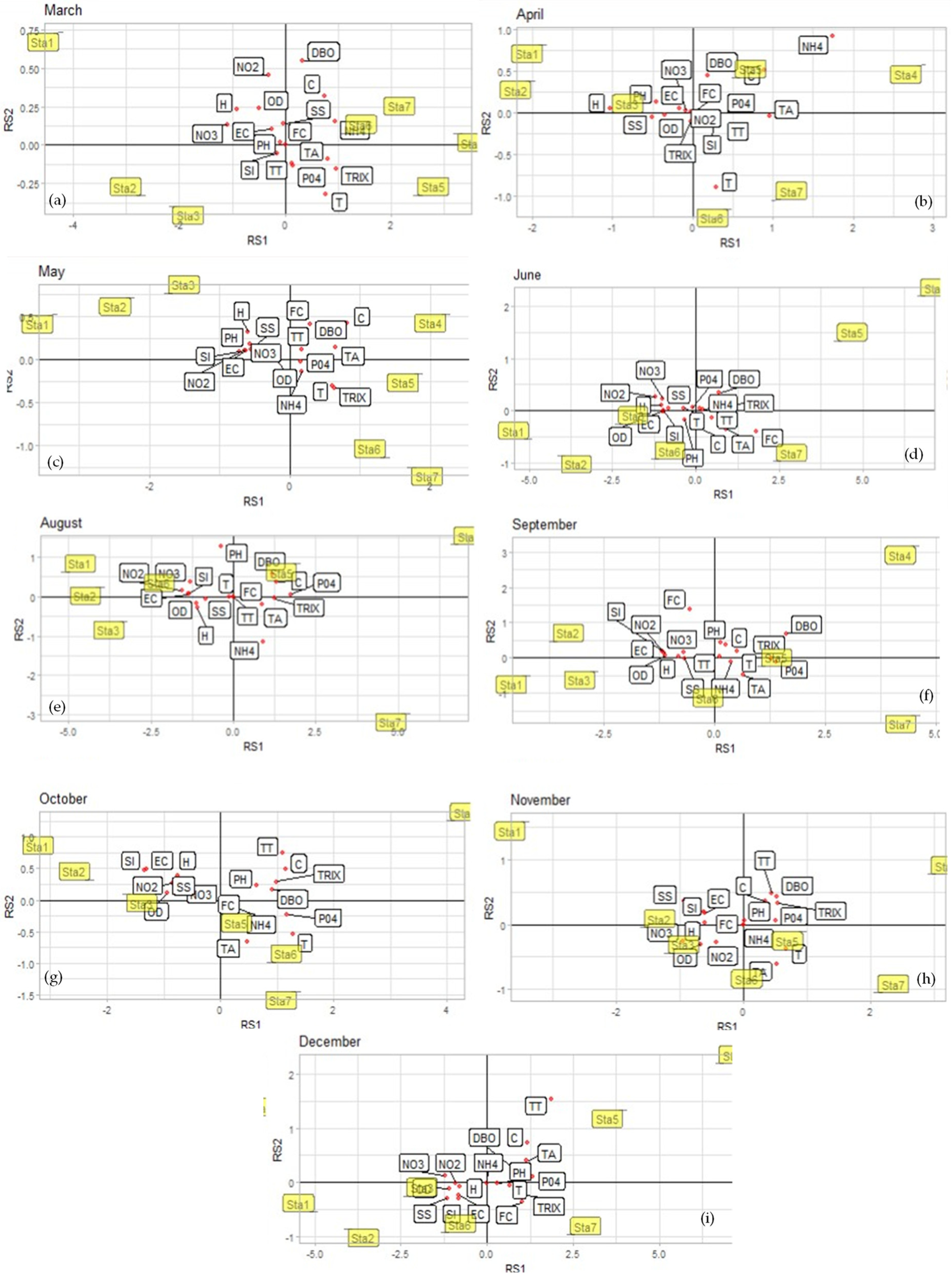
3.3. Intra-Structure Analysis

In this step, we intend to interpret the compromise space through the correlations of the original variables with the dimensions of compromise over the months (Figure 5).

Table A6. Coordinates of dimensions 1 and 2.

Months	Variable	Dim 1	Dim 2
March	NO3−	−1083	0.110
	TRIX	0.958	−0.178
	NH4+	0.937	0.145
	H	−0.912	0.232
	TA	0.808	−0.092
April	NH4+	1737	0.920
	H	−1039	0.034
	TA	0.959	−0.053
	C	0.894	0.528
	T	0.302	−0.892
May	C	0.816	0.436
	NO2−	−0.712	0.085
	TA	0.656	0.145
	EC	−0.641	0.104
	TRIX	0.633	−0.325
June	NO2−	−1209	0.263
	H	−1029	0.114
	DO	−1	−0.007
	NO3−	−0.997	0.24
	EC	−0.988	−0.005
August	PO43−	1737	0.072
	NO2−	−1563	0.152
	EC	−1355	0.046
	Sl	−1334	0.06
	C	1316	0.39
September	DBO	1606	0.684
	PO43−	1379	−0.103
	TRIX	1271	−0.016
	Sl	−1194	0.172
	EC	−1191	0.168
October	Sl	−1348	0.46
	EC	−1314	0.477
	T	1276	−0.553
	PO43−	1177	−0.217
	C	1158	0.51
November	NO3−	−0.958	−0.263
	SSs	−0.94	0.353
	T	0.678	−0.373
	DO	−0.669	−0.307
	Sl	−0.619	0.197
December	TT	1848	1542
	PO43−	1333	0.098
	NO3−	−1229	0.121
	C	1171	0.721
	SSs	−1156	−0.284

shows the five variables that contribute the most to the compromise space throughout the months studied.

The three-way analysis method used in this study, specifically partial triadic analysis, inherently involves a certain degree of information compression. This method prioritizes the extraction of the most dominant patterns from a dataset, which can result in the loss of detailed information about specific data points [27,28]. In this regard, the following observations can be drawn from the intra-structure analysis (see also Table A7 and

Table A8. Means ± standard deviation of water indicators by month.

Parameter	Indicator	March	April	May	June	Aug.	Oct.	Nov.	Dec.	Sept.
Inorganic nutrients	NO2− (mg/L)	0.084 ± 0.05	0.0027 ± 0.002	0.069 ± 0.047	0.078 ± 0.085	0.119 ± 0.105	0.06 ± 0.062	0.078 ± 0.034	0.078 ± 0.066	0.11 ± 0.075
	NO3−(mg/L)	0.71 ± 0.41	0.03 ± 0.04	0.24 ± 0.18	0.34 ± 0.35	0.5 ± 0.46	0.11 ± 0.08	0.75 ± 0.32	0.52 ± 0.44	0.26 ± 0.25
	NH4+ (mg/L)	1.04 ± 0.76	1.99 ± 1.38	0.344 ± 0.15	0.397 ± 0.13	0.987 ± 1.17	0.479 ± 0.22	0.017 ± 0.01	0.019 ± 0.01	0.544 ± 0.26
	PO43− (mg/L)	0.35 ± 0.12	0.42 ± 0.21	0.34 ± 0.1	0.52 ± 0.17	2.09 ± 1.06	1.81 ± 0.75	1.07 ± 0.31	2.21 ± 0.84	2 ± 0.86
Chemical indicators	DO (mg/L)	1.46 ± 0.87	1.85 ± 0.52	1.76 ± 0.42	1.44 ± 1.24	2.16 ± 1.49	1.46 ± 1.12	2.01 ± 0.86	1.75 ± 1.69	1.84 ± 1.35
	pH (U-pH)	7.04 ± 0.04	7.72 ± 0.12	7.73 ± 0.14	7.6 ± 0.07	7.54 ± 0.16	7.65 ± 0.11	7.33 ± 0.04	7.74 ± 0.08	7.48 ± 0.12
	BOD (mg/L)	14.12 ± 5.4	12.47 ± 4.27	8.48 ± 4.87	10.02 ± 6.5	15.11 ± 10.92	9.83 ± 7.64	11.63 ± 5.5	11.86 ± 6.23	17.72 ± 15.07
	TA (mg/L)	144.4 ± 15.92	146.69 ± 18.89	142.16 ± 12.54	151.22 ± 17.63	144.43 ± 17.19	149.01 ± 14.33	141.82 ± 15.47	165.75 ± 23.67	148.95 ± 13.93
	TH (mg/L)	717.72 ± 286.67	596.75 ± 320.5	884.18 ± 248.12	746.1 ± 344.25	995.93 ± 397.66	978.98 ± 290.1	1552.56 ± 226.91	1358.94 ± 248.72	1003.5 ± 283.24
	SI (mg/L)	5.11 ± 1.57	4.45 ± 1.38	8.78 ± 3.42	11.02 ± 4.47	12.93 ± 6.1	15.35 ± 6.53	20.8 ± 3.78	20.43 ± 3.98	14.9 ± 5.66
Physical indicators	TT (NTU)	6.25 ± 3.09	21.47 ± 10.72	4.16 ± 3.94	12.01 ± 9.79	2.27 ± 0.96	19.9 ± 24.64	8.22 ± 13.08	31.92 ± 44.3	3.4 ± 2.19
	C (mg/L)	143.43 ± 99.97	163.14 ± 128.26	160.29 ± 114.12	97.43 ± 44.97	253.29 ± 170.47	199.71 ± 158.46	46 ± 67.07	199.57 ± 174.93	76.5 ± 63.19
	SSs (mg/L)	82 ± 9.09	63.29 ± 16.51	116.14 ± 16.97	110.29 ± 27.38	120.29 ± 36.16	147.14 ± 39.29	167.86 ± 35.48	174.86 ± 36.09	133.21 ± 27.68
	T (°C)	27.86 ± 0.56	28.06 ± 0.79	27.83 ± 0.45	26.84 ± 0.44	26.69 ± 0.71	26.64 ± 0.94	26.83 ± 0.54	26.94 ± 0.45	26.34 ± 0.48
	EC	159.59 ± 47.71	83.06 ± 48.92	282.53 ± 100.23	347.1 ± 129.87	401.06 ± 178.66	466.64 ± 185.27	621.22 ± 102.94	610.92 ± 110.64	458.55 ± 162.82
Contamination indicator	TRIX	7.87 ± 0.69	7.47 ± 0.13	7.21 ± 0.38	7.35 ± 0.17	8.2 ± 0.65	8.2 ± 0.58	7.58 ± 0.4	8.39 ± 0.62	8.43 ± 0.68

).

In March, elevated concentrations of NO₃⁻ and hardness are observed at station 1, station 7 exhibits high levels of TRIX, temperature, and total alkalinity, and station 4 records elevated NH₄⁺ levels (Figure 5a).

April’s data reveal increased concentrations of color, NH₄⁺, and total alkalinity at station 4, elevated temperatures at stations 6 and 7, and higher levels of hardness and suspended solids at station 1 (Figure 5b).

May’s data indicate elevated concentrations of color and alkalinity at station 4, with high levels of NO₂⁻ and electric conductivity observed at stations 1, 2, and 3. Additionally, stations 6 and 7 exhibit elevated levels of TRIX (Figure 5c).

In June, station 1 records high levels of NO₂⁻, hardness, dissolved oxygen, electrical conductivity, and NO₃⁻ (Figure 5d).

August’s data highlight higher concentrations of PO₄³⁻ and color at station 4, along with elevated levels of NO₂⁻, electric conductivity, and salinity at station 1 (Figure 5e).

September’s data reflect elevated concentrations of BOD and color at station 4, PO₄³⁻ and TRIX levels elevated at stations 7 and 4, and electric conductivity and salinity heightened at stations 1 and 2 (Figure 5f).

In October, elevated concentrations of electric conductivity and salinity are observed at stations 1 and 2, with high temperatures recorded at stations 7, 6, and 4. Additionally, station 4 exhibits high levels of color and PO₄³⁻ (Figure 5g).

November’s data reveal elevated concentrations of NO₃⁻, salinity, dissolved oxygen, and suspended solids at station 1, with high temperatures observed at station 7 (Figure 5h).

In December, high turbidity values, along with elevated concentrations of PO₄³⁻ and color, are observed at stations 4 and 5. Station 1 records elevated levels of NO₃⁻, while suspended solids are noted at stations 1 and 2 (Figure 5i).

Despite the growing interest and utility of new multivariate statistical methods, the application of the PTA method may have certain limitations. Our data possess a triadic structure (stations, months, and physicochemical parameters), which is common in environmental studies, allowing for the simultaneous analysis of the interactions among these three dimensions. Additionally, the applied method preserves the structure and integrity of the original data. However, PTA may face challenges in its integration into different contexts due to computational complexity (especially with large datasets), its dependence on high-quality input data (e.g., missing data, scales, and coding of variables), and the requirement for prior knowledge in principal component analysis [14,16,35].

4. Conclusions

The STATIS family analysis and the three-way multivariant methods were a challenging task in the research. However, precise answers have been provided to the research questions set. Firstly, it was feasible to demonstrate the relationships that occur between the properties of water, allowing us to observe their impact on its quality. Secondly, restrictions related to water properties were identified. These restrictions made it possible to characterize the stations that had values higher and lower than the average recorded for each variable over time. The partial triadic analysis allowed us to discover that the fourth station had higher values of certain indicators, such as NH₄⁺, alkalinity, color, PO₄³⁻, BOD, TRIX, and turbidity, with variations in their intensity throughout the months. The fifth station showed similar behavior, but with reduced intensity. Regarding the TRIX, its value was higher for stations 4, 7, 5, and 6.

Stations 1, 2 and 3 were characterized by higher average values of NO₂⁻, NO₃⁻, electrical conductivity, salinity, and suspended solids. Station 7 was distinguished by haying higher temperatures compared to the other stations during the months of March, April, May, October, and November. The levels at station 6 resembled those at station 7 in some months. During March and April, NH₄⁺ presented a greater contribution compared to the other months. In June, variables such as NO₂, hardness, liquid oxygen, NO₃⁻, and electrical conductivity predominated, which arose on the lower side of the analysis. These insights can explain the worsening of common structures. Furthermore, partial triadic analysis method offered a profound understanding of 86% of the variability. This information reveals a relationship of contamination between different months of the year and different properties of water. This relationship allows us to identify observations that arise both on top and on average. This emphasis on specific stations helps us to discern significant patrons and better understand how the characteristics of the water fluctuate over time.

In conclusion, the detailed analysis of sample stations allowed us to identify specific trends and behaviors in the properties of water, providing an integral vision of how these factors affect the quality of water at different times of the year. This information is crucial for the management and conservation of water supplies, as it allows one to implement more effective measures adapted to the specific needs of each station and period.

References

1. Mosquera, M.N.R.; Criollo, D.A.R. El Estero Salado en el desarrollo urbano de Guayaquil: Crónicas de un recurso natural en decadencia. In Seminario Internacional de Investigación en Urbanismo; Universitat Politècnica de Catalunya: Barcelona, Spain, 2019. [Google Scholar]
2. Dudgeon, D.; Arthington, A.H.; Gessner, M.O.; Kawabata, Z.I.; Knowler, D.J.; Lévêque, C.; Naiman, R.J.; Prieur-Richard, A.H.; Soto, D.; Stiassny, M.L.J.; et al. Freshwater biodiversity: Importance, threats, status and conservation challenges. Biol. Rev. Camb. Philos. Soc. 2006, 81, 163–182. [Google Scholar] [CrossRef]
3. Zambrano, N. Plan de Manejo del Bosque Protector Estero Salado Norte. In Programa de Manejo de Recursos Costeros; PMRC: Athens, GA, USA, 2007; 79p. [Google Scholar]
4. Monserrate, L.; Medina, J.F.; Calle, P. Estudio de Condiciones Físicas, Químicas y Biológicas en la zona Intermareal de dos Sectores del Estero Salado con Diferente Desarrollo Urbano; Escuela Superior Politécnica del Litoral, ESPOL: Guayaquil, Ecuador, 2011. [Google Scholar]
5. Villacis, J.E.R.; Gavilánez, L.H.; Huilcapi, C.S.; Alvarado, H.M.A.; García, R.S.M.; Larreta, F.S.G.; Santi, W.M. Evaluación de la contaminación físico-química y microbiológica de aguas del estero salado. Dominio Cienc. 2017, 3, 672–691. [Google Scholar]
6. Distrital, A.A. Norma Técnica para el Control de Descargas Líquidas; Cámara de Industrias y Producción: Quito, Ecuador, 2013. [Google Scholar]
7. Vollenweider, F.X.; Vollenweider-Scherpenhuyzen, M.F.; Bäbler, A.; Vogel, H.; Hell, D. Psilocybin induces schizophrenia-like psychosis in humans via a serotonin-2 agonist action. Neuroreport 1998, 9, 3897–3902. [Google Scholar] [CrossRef]
8. Gourdol, L.; Hissler, C.; Hoffmann, L.; Pfister, L. On the potential for the Partial Triadic Analysis to grasp the spatio-temporal variability of groundwater hydrochemistry. Appl. Geochem. 2013, 39, 93–107. [Google Scholar] [CrossRef]
9. Mendes, S.; Fernández-Gómez, M.J.; Pereira, M.; Azeiteiro, U.; Galindo-Villardón, M.P. The efficiency of the Partial Triadic Analysis method: An ecological application. Biom. Lett. 2010, 47, 83–106. [Google Scholar]
10. Thioulouse, J.; Simier, M.; Chessel, D. Simultaneous analysis of a sequence of paired ecological tables. Ecology 2004, 85, 272–283. [Google Scholar] [CrossRef]
11. Rossi, J.P. The spatiotemporal pattern of a tropical earthworm species assemblage and its relationship with soil structure: The 7th international symposium on earthworm ecology·Cardiff·Wales·2002. Pedobiologia 2003, 47, 497–503. [Google Scholar]
12. Rossi, J.P.; Nardin, M.; Godefroid, M.; Ruiz-Diaz, M.; Sergent, A.S.; Martinez-Meier, A.; Paques, L.; Rozenberg, P. Dissecting the space-time structure of tree-ring datasets using the partial triadic analysis. PLoS ONE 2014, 9, e108332. [Google Scholar] [CrossRef] [PubMed]
13. Marco, C.; Fenga, L. Assessing Partial Triadic Analysis with MaximumEntropy Bootstrap: An Application to BES Italianeducation Indicators. preprint 2021, 21. [Google Scholar] [CrossRef]
14. Bertrand, F.; Maumy, M. Using Partial Triadic Analysis for Depicting the Temporal Evolution of Spatial Structures: Assessing Phytoplankton Structure and Succession in a Water Reservoir. Case Stud. Bus. Ind. Gov. Stat. 2010, 4, 23–43. [Google Scholar]
15. Prieto, J.M.; Amor, V.; Turias, I.; Almorza, D.; Piniella, F. Evaluation of Paris MoU Maritime Inspections Using a STATIS Approach. Mathematics 2021, 9, 2092. [Google Scholar] [CrossRef]
16. Misztal, M. Application of the Partial Triadic Analysis Method to Analyze the Crime Rate in Poland in the Years 2000–2017. Folia Oeconomica Stetin. 2020, 20, 249–278. [Google Scholar] [CrossRef]
17. Rodríguez-Rosa, M.; Gallego-Álvarez, I.; Vicente-Galindo, P.; Galindo-Villardón, M.P. Are Social, Economic and Environmental Well-Being Equally Important in all Countries around the World? A Study by Income Levels. Soc. Indic. Res. 2017, 131, 543–565. [Google Scholar] [CrossRef]
18. García-Bustos, S.; Ruiz-Barzola, O.; Morán, M.; Tandazo, W. Método XSTATIS para estudio de las principales causas de muerte en Ecuador 2020. Papeles Población 2024, 29, 53–81. [Google Scholar] [CrossRef]
19. Prieto, J.M.; Amor-Esteban, V.; Almorza-Gomar, D.; Turias, I.; Piniella, F. Application of Multivariate Statistical Techniques as an Indicator of Variability of the Effects of COVID-19 on the Paris Memorandum of Understanding on Port State Control. Mathematics 2023, 11, 3188. [Google Scholar] [CrossRef]
20. Darwiche-Criado, N.; Comín, F.A.; Jiménez, J.J.; Masip, A.; García, M.; Eismann, S.G.; Sorando, R. Restoring wetlands to remove agricultural pollution in surface waters: Assessment and monitoring through partial triadic analysis (PTA). In Proceedings of the 9th Symposium for European Freshwater Sciences, Geneva, Switzerland, 5–10 July 2015; Volume 2, p. 4. [Google Scholar]
21. Jiménez, J.J.; Darwiche-Criado, N.; Sorando, R.; Comín, F.A.; Sánchez-Pérez, J.M. A Methodological Approach for Spatiotemporally Analyzing Water-Polluting Effluents in Agricultural Landscapes Using Partial Triadic Analysis. J. Environ. Qual. 2015, 44, 1617–1630. [Google Scholar] [CrossRef] [PubMed]
22. Slimani, N.; Jiménez, J.J.; Guilbert, E.; Boumaïza, M.; Thioulouse, J. Surface water quality assessment in a semiarid Mediterranean region (Medjerda, Northern Tunisia) using partial triadic analysis. Environ. Sci. Pollut. Res. 2020, 27, 30190–30198. [Google Scholar] [CrossRef] [PubMed]
23. Cedeño, J.; Donoso, M.C. Atlas Pluviométrico del Ecuador, 1st ed.; Programa Hidrológico Internacional de la UNESCO para América Latina y el Caribe: Guayaquil, Ecuador, 2010; pp. 1–86. [Google Scholar]
24. NTE INEN 2176; Agua. Calidad del Agua. Muestreo. Técnicas de Muestreo. INEN: Quito, Ecuador, 2019.
25. APHA. Standard Methods for the Examination of Water and Wastewater, 21st ed.; American Public Health Association/American Water Works Association/Water Environment Federation: Washington, DC, USA, 2005. [Google Scholar]
26. NTE INEN 2169:2013; Agua. Calidad del Agua. Muestreo. Manejo y Conservación de Muestras. INEN: Quito, Ecuador, 2013.
27. Abdi, A.; Williams, L.; Valentin, D.; Bennani-Dosse, M. STATIS and DISTATIS: Optimum multitable principal component analysis and three way metric multidimensional scaling. Wiley Interdiscip. Rev. Comput. Stat. 2012, 6, 124–167. [Google Scholar] [CrossRef]
28. Lavit, C.; Escoufier, Y.; Sabatier, R.; Traissac, P. The ACT (STATIS method). Comput. Stat. Data Anal. 1994, 8, 97–119. [Google Scholar] [CrossRef]
29. Jaffrenou, P.; Malécot, G. Sur l’analyse des Familles Finies de Variables Vectorielles: Bases Algébriques et Application à la Description Statistique; Éditeur non Identifié. 1978. Available online: https://three-mode.leidenuniv.nl/bibliogr/jaffrennoupa_thesis/jaffrennoupa1978.pdf (accessed on 22 July 2024).
30. Rodríguez-Martínez, C.C.; Cubilla-Montilla, M.; Vicente-Galindo, P.; Galindo-Villardón, P. X-STATIS: A Multivariate Approach to Characterize the Evolution of E-Participation, from a Global Perspective. Mathematics 2023, 11, 1492. [Google Scholar] [CrossRef]
31. Robert, P.; Escoufier, Y. A Unifying Tool for Linear Multivariate Statistical Methods: The RV-Coefficient. J. R. Stat. Soc. Ser. C Appl. Stat. 1976, 25, 257–265. [Google Scholar] [CrossRef]
32. Dray, S.; Dufour, A.B. The ade4 Package: Implementing the Duality Diagram for Ecologists. J. Stat. Softw. 2007, 22, 1–20. [Google Scholar] [CrossRef]
33. Durmishi, N.; Xhabiri, G.; Ferati, I.; Alija, D.; Karakashova, L.; Stamatovska, V.; Lazova-Borisova, I. Monitoring of some parameters of quality and microbiological safety in drinking water. J. Food Technol. Nutr. 2023, 6, 2023. [Google Scholar]
34. Fiori, E.; Zavatarelli, M.; Nadia, P.; Mazziotti, C.; Ferrari, C. Observed and simulated trophic index (TRIX) values for the Adriatic Sea basin. Nat. Hazards Earth Syst. Sci. 2016, 16, 2043–2054. [Google Scholar] [CrossRef]
35. Aibar, G.B.; Monteiro, S.D.F.; Somohano-Rodríguez, F.M. The Waste Hierarchy at the Business Level: An International Outlook. Mathematics 2023, 11, 4574. [Google Scholar] [CrossRef]
Figure 1. Location of control stations in the terminal segment of the Estero Salado.
Water 16 02196 g001
Figure 2. Partial triadic analysis.
Water 16 02196 g002
Figure 3. Projection of the nine periods onto the first and second components (inter-structure).
Water 16 02196 g003
Figure 4. Simultaneous representation of the stations and water indicators in plans 1 and 2 (compromise).
Water 16 02196 g004
Figure 5. Partial factorial scores and variable loadings for the first two dimensions of the compromise space (intra-structure): (a) March representations; (b) April representations; (c) May representations; (d) June representations; (e) August representations; (f) September representations; (g) October representations; (h) November representations; (i) December representations.
Water 16 02196 g005