Article

Evaluation of Future Changes in Climate Extremes over Southeast Asia Using Downscaled CMIP6 GCM Projections

School of Civil and Environmental Engineering, Nanyang Technological University, 50 Nanyang Ave, Singapore 639798, Singapore
*
Author to whom correspondence should be addressed.
Water 2024, 16(15), 2207; https://doi.org/10.3390/w16152207
Submission received: 26 June 2024 / Revised: 31 July 2024 / Accepted: 2 August 2024 / Published: 4 August 2024
(This article belongs to the Special Issue Analysis of Extreme Precipitation under Climate Change)

Abstract

:
This study presented an assessment of climate extremes in the Southeast Asia (SEA) region, utilizing downscaled climate projections from the Coupled Model Intercomparison Project Phase 6 (CMIP6) Global Climate Models (GCMs). The study outputs uncovered statistically significant trends indicating a rise in extreme precipitation and temperature events throughout SEA for both the near-term (2021–2060) and long-term (2061–2100) future under both SSP245 and SSP585 scenarios, in comparison to the historical period (1950–2014). Moreover, we investigated the seasonal fluctuations in rainfall and temperature distributions, accentuating the occurrence of drier dry seasons and wetter rainy seasons in particular geographic areas. The focused examination of seven prominent cities in SEA underscored the escalating frequency of extreme rainfall events and rising temperatures, heightening the urban vulnerability to urban flooding and heatwaves. This study’s findings enhance our comprehension of potential climate extremes in SEA, providing valuable insights to inform climate adaptation, mitigation strategies, and natural disaster preparedness efforts within the region.

1. Introduction

Human activities are causing a persistent increase in greenhouse gas emissions, which has raised apprehensions about the growing occurrence and severity of extreme weather phenomena across the globe. It is of utmost significance to comprehend the prospective alterations in extreme climate events for developing effective approaches for addressing both adaptation and mitigation of the consequences of climate change in the area. To address this issue, numerous studies have utilized the general circulation models (GCMs) to predict climate change under different greenhouse gas and economic activity scenarios [1,2,3,4,5]. The Coupled Model Intercomparison Project Phase 6 (CMIP6) signifies the latest generation of GCMs, providing more comprehensive and various climate projections by combining the representative concentration pathways (RCPs) with shared socioeconomic pathways (SSPs). CMIP6 GCMs provide improved spatial and temporal resolutions, facilitating a more comprehensive evaluation of regional climate changes. They have been observed to surpass their predecessors from the CMIP5 dataset [6,7,8,9].
The original GCMs were typically generated with coarse resolutions and with significant divergence among models [10], posing limitations in capturing regional and local climate characteristics effectively. Previous studies have utilized low-resolution original CMIP5 and CMIP6 GCMs of future climate change projections with spatial resolution ≥0.5° [3,9,11,12,13,14,15]. High-resolution climate data availability with spatial resolution ≤0.25° is essential for conducting thorough and localized examinations of the impact of climate change in particular regions [16]. Downscaling is primarily required to depict small-scale climate conditions by identifying vulnerable areas to be potentially influenced by climate change impacts. There are various techniques to downscale the outputs from GCMs; the commonly used methods are statistical and dynamic downscaling approaches. Dynamical downscaling efforts entail employing Regional Climate Models (RCMs), which utilize the output from GCMs as both boundary and initial conditions. Nevertheless, this process demands significant computational resources and is computationally intensive [17]. An alternative approach to this is statistical downscaling, which involves establishing a link between global climate variables and regional or local characteristics to generate high-resolution climate data [18]. Generally, the statistical approach can be carried out with lower computational cost.
Southeast Asia (SEA) is particularly situated in a region highly susceptible to the impacts of climate extremes [11,12,13,19]. The climate variability in SEA is intricately tied to the El Niño/Southern Oscillation (ENSO) phenomenon [20,21,22]. Precipitation and temperature play pivotal roles in contributing to the incidence of floods and droughts in the SEA region. Excessive rainfall can lead to flooding as it saturates the soil and disrupts natural drainage patterns. Prolonged spells of heavy storms and severe heat can also lead to drought problems, exacerbating water scarcity issues, with a primary impact on agricultural systems in this region. Agriculture, covering 30% of the overall land area of SEA, bears the brunt of these challenges [23].
Previously, many studies have investigated the historical climate extremes, including precipitation and temperature indices, in mainland SEA [3,19,24,25] along with the entire SEA [26,27,28,29,30]. These earlier studies predominantly utilized CMIP5 scenarios as their primary basis for research [27,31]. In the Southeast Asian context, many researchers have undertaken the assessment of CMIP6 GCMs for climate projections. Ge et al. [13] employed data generated by fifteen climate models from CMIP6 to forecast precipitation levels in SEA by the conclusion of the 21st century. Liu et al. [32] assessed the performance ranking of CMIP6 GCMs for rainfall projection in SEA. Ly et al. [33] and Try et al. [9] simulated flood extreme events under climatic change projections using the CMIP6 GCMs in the Mekong River Basin.
Nevertheless, these studies utilized the original coarse resolution of GCMs, making it difficult to capture the characteristics of small, specific regions. There remains a gap in the evaluation of climate change extremes within the SEA region, using downscaled GCMs with high resolution capable of capturing precise local conditions. Moreover, with its inclusion of many sprawling and densely populated cities like Bangkok, Hanoi, Jakarta, and Kuala Lumpur, SEA faces heightened vulnerability to the consequences of urban flooding. Previous studies have touched upon this matter and highlighted that SEA underwent rapid development, making their city prone to urban flooding and necessitating strategies to mitigate extreme urban floods in this region, for instance, case studies of cities in Thailand [34,35], Vietnam [36,37], Cambodia [38,39], Myanmar [40,41], Indonesia [42,43], and the Philippines [44,45]. However, there has not been detailed information about the projection of urban flood hazards under the impacts of climate change in these cities yet. Therefore, there is a pressing need for a more comprehensive investigation focused on urban areas in SEA, utilizing the latest insights from downscaled CMIP6 GCMs.
Hence, this study aims to evaluate the predictability of historical climate datasets in SEA and investigate the climate change impact on precipitation and temperature concerning both wet and dry extreme events in this region. We utilize bias-adjusted projections sourced from the NASA Earth Exchange Global Daily Downscaled Projections (NEX-GDDP-CMIP6), which are derived from GCMs. The study will provide a comprehensive analysis of alterations in the timing and geographical spread of extreme precipitation and temperature. Section 2 will describe the study area, datasets, and climate extreme analysis and indicators. Section 3 will present the outputs of precipitation and temperature changes, including their spatial and temporal distribution, together with an analysis of frequency changes in some local SEA cities. Finally, in Section 4, we will discuss the overall findings and draw conclusions.

2. Data and Methods

2.1. Study Area

This research centers on the SEA region, characterized by its multifaceted populations and unique geographical positioning at the crossroads of the Indian Ocean and the Pacific Ocean (Figure 1). The inhabitants in this region have a history of enduring substantial riverine and coastal floods. For instance, the Chao Phraya flooding event in 2011 witnessed an unprecedented amount of rainfall that was 1.2 times higher than the previous major event in Thailand [46]. In the year 2000, extensive flooding occurred in the Lower Mekong floodplain and delta, primarily affecting Cambodia, Lao PDR, Thailand, and Vietnam, resulting in an economic loss amounting to USD 517 million [9,47]. Furthermore, major cities in SEA experienced significant urban flooding, including Jakarta in Indonesia [48], Manila in the Philippines [49], Bangkok in Thailand [50], Phnom Penh in Cambodia [38], Kuala Lumpur in Malaysia [51], and Ho Chi Minh in Vietnam [52]. Figure 1 illustrates the area of study, comprising five primary regions defined for assessing regional variations in future precipitation and temperature projections. These regions include Mainland Southeast Asia (MSEA), Sumatra and the Malay Peninsula (SRMP), Java Island (JAVA), Borneo and Sulawesi Islands (BORS), and the Philippines (PHLP) [28].

2.2. Datasets and Indices

To assess past climate conditions, this research utilized precipitation data from the Asian Precipitation—Highly Resolved Observational Data Integration Towards Evaluation of Water Resources (APHRODITE) [53]. The APHRODITE dataset was constructed by sourcing a concentrated network of rainfall measurements from rain gauges across Asia at a daily resolution of 0.25° × 0.25° available from 1951 to 2015. Many research studies across Asia have extensively utilized this dataset [2,3,54,55,56]. Additionally, we employed minimum and maximum daily temperature data obtained via the Global Unified Temperature dataset supplied by the National Oceanic and Atmospheric Administration (NOAA) Climate Prediction Center (CPC) [57]. This dataset was created through the integration of various available products, thereby improving its quality and ensuring consistency via an optimal interpolation objective analysis technique. It offers a global daily resolution of 0.5° × 0.5° incorporating the period since 1979. Numerous research initiatives have made extensive use of this dataset [57,58,59,60].
For future climate data, this study employed the climate projection dataset provided by NEX-GDDP-CMIP6 [4], accessible at https://nex-gddp-cmip6.s3.us-west-2.amazonaws.com/index.html (accessed on 30 May 2023). This dataset offers a comprehensive compilation of precise climate change predictions that have been downscaled and bias-corrected with the Bias-Correction Spatial Disaggregation (BCSD) method [61,62]. It enables the evaluation of potential climate change impact on phenomena influenced by intricate climate variations and local terrain influences on weather conditions. This dataset has a fine spatiotemporal resolution (daily and 0.25° × 0.25°) covering the historical period of 1950–2014 and future projection period 2015–2100. Two future project scenarios from CMIP6, namely, SSP245 and SSP585, were used for analysis. The variables of daily precipitation, maximum temperature, and minimum temperature were extracted for SEA region from 29 GCMs provided by various agencies across 14 different regions [4]. A full list of these GCMs can be referred to Supplementary Materials.
Following the definitions by Zhang et al. [63], this research utilized four precipitation indices for extreme wet (two) and dry climates (two): maximum precipitation at daily scale (RX1day), number of days when precipitation exceeds 20 mm/day (R20), daily precipitation value at the 99th percentile (R99P), and maximum length of successive days with rainfall amount below 1 mm (CDD) [63]. In addition, four indicators of hot and cold conditions derived from daily maximum (Tmax) and minimum temperatures (Tmin) are also used: annual peak of Tmax (TXmax), 90th percentile of Tmax (Tmax90P), annual lowest value of Tmin (TNmin), and 10th percentile of Tmin (Tmin10P). A list of the extreme climate indicators is also provided in Supplementary Materials. Indices without percentiles were derived on an annual basis and subsequently averaged to obtain the climatological mean. Conversely, indicators with percentiles (i.e., R99P, Tmax90P, and Tmin10P) were calculated using the data distributions spanning the entire analyzed periods.

2.3. Statistical Test and Indicators

2.3.1. K-S Two Parameter Test

The Kolmogorov–Smirnov (K–S) test, which could measure the statistical variability between two groups of samples, is employed to assess the alterations of precipitation and temperature distribution patterns between historical and projected future climates. The greatest disparity in the cumulative distribution functions (CDFs) of two groups of samples is written as [64]:
D n , m = sup x F n x F m x
where F n and F m represent the empirical CDFs of the two datasets, while “sup” denotes the supremum function. The null hypothesis ( H 0 ) posits that no notable distinction exists between the two CDFs. To reject the null hypothesis, the probability of the samples’ distributions must surpass the designated significance threshold [64].

2.3.2. Extreme Value Analysis

The Generalized Extreme Value (GEV) distribution is commonly employed for fitting climate extreme events based on three parameters. The relevant probability density function (PDF) is written as [65]:
F x ; μ , σ , ξ = exp 1 + ξ ( x μ σ ) 1 ξ
where μ , σ , and ξ denote the location, scale, and shape parameters, respectively.

2.3.3. SPAEF Index

SPAtial EFficiency metric (SPAEF) is an indicator of evaluating spatial agreement by integrating three independent metrics into one [66]. In this research, it is utilized to contrast spatial precipitation and temperature maps among the NEX-GDDP-CMIP6 GCMs, as delineated by the subsequent equation [66]:
SPAEF = 1 ( A 1 ) 2 + ( B 1 ) 2 + ( C 1 ) 2
where A is Pearson correlation [67]; B and C are metrics for bias and variability. The detailed definition of A, B, and C can be referred to Try et al. [9]. SPAEF can range from to 1, where 1 indicates the highest spatial similarity between the two datasets.

2.3.4. FSS Index

The Fractions Skill Score (FSS) is a measurement of spatial agreement between the two geographic maps ranging from 0 to 1 [68], where 1 is the best matching among the two datasets. It is given by:
FSS = M S E ( n ) M S E ( n ) r e f
where M S E and M S E r e f are the mean square error calculated by the following equations [66]:
M S E ( n ) = 1 N x N y i = 1 N x j = 1 N y O n i , j M n i , j 2
M S E ( n ) r e f = 1 N x N y i = 1 N x j = 1 N y O n i , j 2 + i = 1 N x j = 1 N y M n i , j 2
where N x and N y are the numbers of columns and rows in the geospatial map of reference ( O ) , respectively, and NEX-GDDP-CMIP6 ( M ) is characterized by its own number of columns and rows.

2.3.5. Analysis Procedure

The NEX-GDDP-CMIP6 dataset was first evaluated by comparing its rainfall data with APHRODITE and its temperature data with CPC. This comparison ensures the dataset’s accuracy and reliability against established observational records. After verifying the historical climate simulations of extreme precipitation and temperature, the research proceeded to examine future projections to assess how their characteristics might evolve. Future time frames, including two projection scenarios, SSP245 and SSP585, were investigated. The study compared precipitation anomalies for all four precipitation indices across five regions in the SEA for both the short-term future (2021–2060) and the long-term future (2061–2100) against the baseline period of 1950–2014.
We have further broadened our research scope to encompass the distinctive climatic characteristics of several prominent cities in SEA, encompassing Bangkok, Hanoi, Jakarta, Kuala Lumpur, Manila, Phnom Penh, and Singapore. Our goal is to investigate extreme weather occurrences associated with specific return periods determined through fitting GEV curves. We have extracted climatological data for each city and its suburban areas using 3 × 3 grid cells from NEX-GDDP-CMIP6 dataset. Our analysis focuses on variations in the annual maximum series (AMS) of precipitation and temperature at daily scale with 2-, 10-, 50-, and 100-year return periods. We draw comparisons between the historical climate patterns and future predictions based on two scenarios, namely SSP245 and SSP585. Lastly, we conducted an examination of extreme temperatures in the seven cities by analyzing their daily AMS and GEV fitting curves.

3. Results

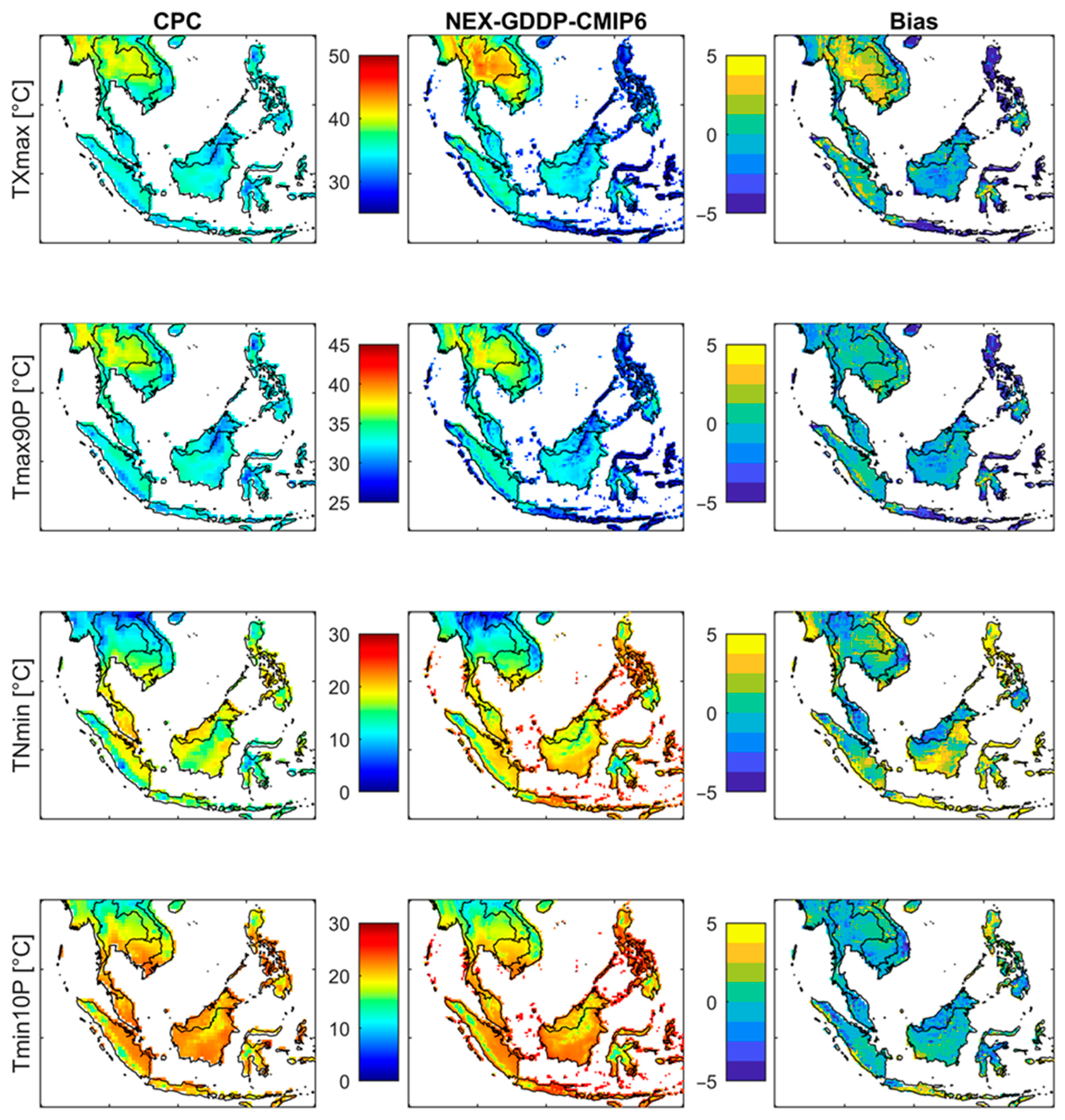
3.1. Historical Verification

The performance evaluation of the historical simulation of 29 GCMs from NEX-GDDP-CMIP6 was assessed by the comparison of the ensemble mean with reference datasets of APHRODITE precipitation and CPC temperature. Figure 2 shows the spatial comparison of four precipitation indicators (RX1day, R20, R99P, and CDD) obtained from the NEX-GDDP-CMIP6 ensemble mean over the 1951–2014 period and APHTODITE during 1951–2014. A bias map is also shown based on the difference between ensemble mean and reference. For RX1day, both datasets exhibited a generally similar distribution pattern, yielding SPAEF and FSS scores of 0.62 and 0.91, respectively. However, there was notable underestimation in the Philippines, contrasted by overestimation in Central Vietnam and Southwestern Cambodia. The NEX-GDDP-CMIP6 dataset exhibited a slight overestimation of the R20 index in the Northern Philippines, Southwestern Cambodia, and the coastal areas in the west of Myanmar and Thailand, with an overall SPAEF of 0.49 and FSS of 0.84. In the case of indices R99P and CDD, there was a commendable agreement in spatial distribution across most of the Southeast Asian region, yielding SPAEF scores of 0.59 and 0.70, and FSS scores of 0.94 and 0.97, respectively.
In addition, Figure 3 presents a comparison between the historical NEX-GDDP-CMIP6 dataset for extreme temperatures and the CPC dataset. The spatial patterns do not exhibit significant differences between the two datasets. However, there was an overestimation of TXmax in Thailand and Cambodia within the MSEA region, along with an underestimation in Northern PHLP, resulting in SPAEF = 0.56 and FSS = 0.996. Despite a slight underestimation in JAVA and Northern Philippines for Tmax90P, no significant bias could be observed, with an overall accuracy of SPAEF = 0.71 and FSS = 0.997. On the other hand, the performance of NEX-GDDP-CMIP6 somehow overestimated TNmin for most of the regions in the SEA, particularly in the Northern PHLP, Southeastern BORS, JAVA, and coastal regions of MSEA, yielding accuracy indices of SPAEF = 0.78 and FSS = 0.96. The NEX-GDDP-CMIP6 dataset effectively captured the Tmin10P index for almost all regions across the SEA, with SPAEF = 0.79 and FSS = 0.99.

3.2. Future Projection

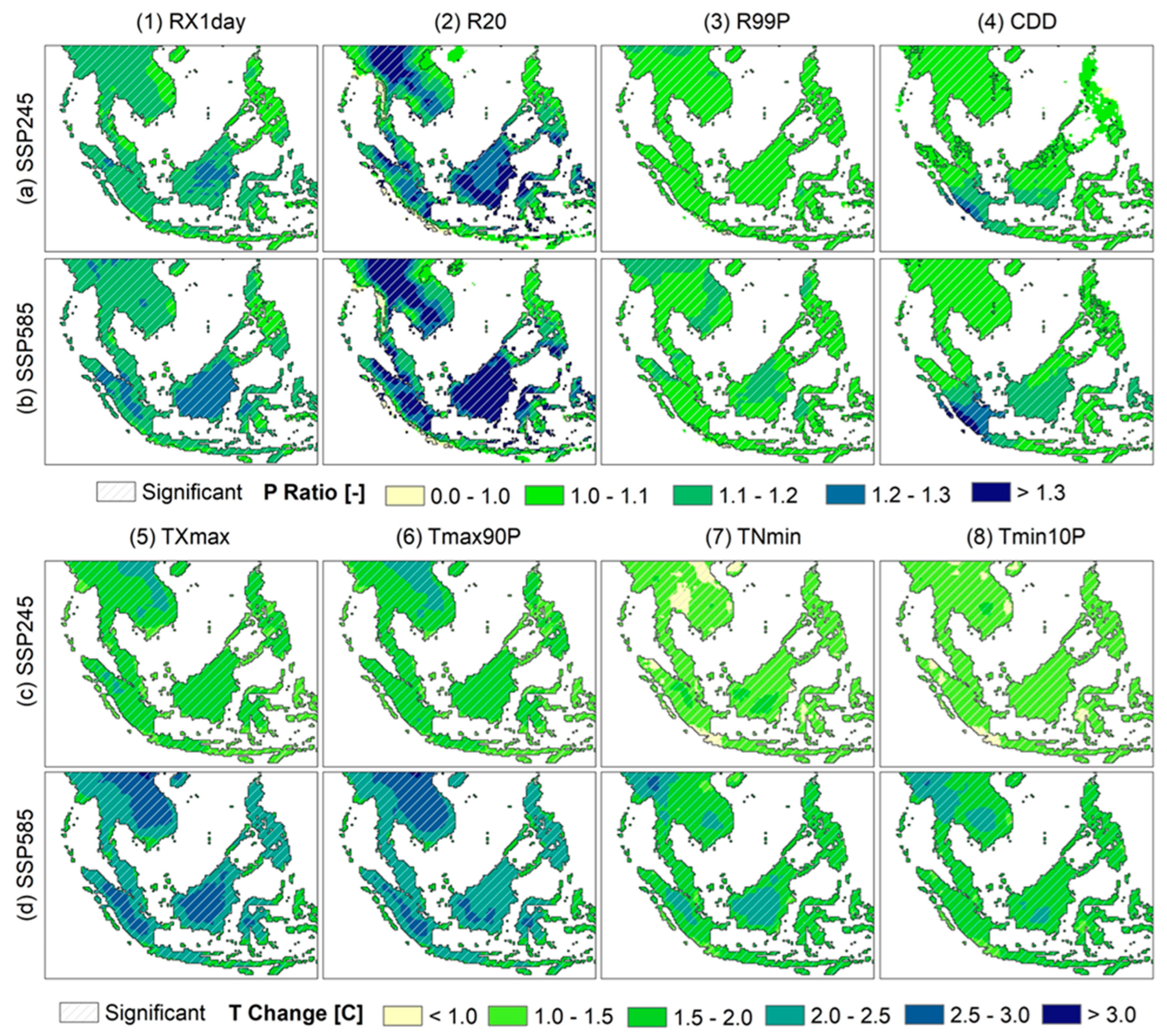
3.2.1. Projection of Precipitation Changes

The indices clearly indicate substantial increases in both projection scenarios for the two projected periods (Table 1). Under the SSP245 scenario, the MSEA region anticipates a rise in the ratio for high extreme rainfall intensity (RX1day and R20) in the range of 1.10 to 1.15 and 1.06 to 1.13, respectively, for the near and far future periods. Conversely, for low rainfall intensity indicators (R99P and CDD), the ratios are expected to be 1.06 to 1.10 and 1.02 for projection periods in the near and far future. In the SRMP, JAVA, and BORS regions, RX1day and R20 are projected to increase by 1.07 to 1.19 and 1.01 to 1.31, with similar increases observed in R99P (1.02 to 1.09) and CDD (1.12 to 1.20). The PHLP region is also expected to experience an increase ranging between 1.08 and 1.12 for high precipitation indices and 1.05 to 1.11 for low precipitation indicators. It is worth noting that almost all extreme precipitation indicators and projected periods demonstrate statistical significance at the 0.1% significant level, with only two cases showing significance at the 1% level, and one case indicating no significance. Furthermore, when considering projections under SSP585, there is a notable increase in precipitation expected over the SEA region compared to SSP245. Specifically, the RX1day and R20 indices are projected to rise significantly, with ratios ranging from 1.07 to 1.14 and 1.03 to 1.20 in the short-term future, and 1.16 to 1.29 and 1.11 to 1.50 in the more distant one, when compared to historical periods. Similarly, the R99 index is anticipated to increase from 1.03 to 1.07 in the near future and from 1.08 to 1.16 in the far future. Additionally, the CDD index is expected to range from 1.02 to 1.18 in the near future and from 1.05 to 1.51 in the far future.
Figure 4a,b spatially illustrates the distribution of precipitation changes, as determined by the ensemble mean of 29 GCMs from the NEX-GDDP-CMIP6 dataset. These changes are observed over the future 65-year periods (2021–2085) when compared to baseline 65-year periods (1950–2014). The spatial patterns mirror the temporal analysis previously discussed for each region within SEA. Notably, we observe clear increases in change ratios across all regions within SEA. The most significant increase is observed in R20, which covers central MSEA and the main island of the BORS region, with a ratio exceeding 1.3. For RX1day, we anticipate an increase of approximately 1.1 to 1.2 for most of the region, and 1.2 to 1.3 for specific areas within the BORS region. Regarding the change ratio for R99P and CDD, we expect it to range between 1.0 and 1.1 for nearly all regions within SEA. It is important to highlight that all four precipitation indices exhibit statistically significant changes to the K-S test, as depicted in Figure 4a,b.

3.2.2. Projection of Temperature Changes

In addition to our analysis of precipitation, this study also delved into temperature changes within SEA. We projected temperature increases for five SEA regions using the ensemble mean derived from 29 downscaled GCMs from the NEX-GDDP-CMIP6 dataset. These projections encompass both the short-term and long-term future of the SSP245 scenario. For TXmax and Tmax90P, we anticipate temperature rises ranging from approximately 1.27 to 2.42 °C and 1.23 to 2.48 °C, respectively (as detailed in Table 2). Meanwhile, TNmin and Tmin10P are predicted to elevate by 0.85 to 1.80 °C and 0.89 to 1.86 °C, respectively, under the SSP245 scenario. In contrast, under SSP585, TXmax is projected to exhibit a notably greater increase, ranging from approximately 1.44 to 1.69 °C in the short-term timeframe and 3.26 to 4.12 °C in the long run. Similarly, Tmax90P is projected to increase by 1.45 to 1.78 °C in the short-term future and 3.26 to 4.09 °C in the long-term one. TNmin is also expected to rise, with an increase ranging from 1.15 to 1.25 °C in the near term and 2.80 to 3.44 °C in the far one, while Tmin10P shows a range of increases between 1.13 to 1.25 and between 2.74 to 3.51 °C in the short- and long-term future, respectively. It is essential to recognize that the statistical significance of these temperature projections, as assessed by the K-S test, is evident for all five regions and both projection scenarios, with significance observed at the 0.1% level (as summarized in Table 2).
Figure 4c,d illustrates the spatial variation of temperature changes in the distant future (2021–2085) in comparison to those in the baseline period (1950–2014). Notably, there is a significant contrast between the two projection scenarios, SSP245 and SSP585. Under the SSP245, most areas within SEA are anticipated to witness a general temperature rise at approximately 1.5 to 2.0 °C for TXmax and Tmax90P, and 1.0 to 1.5 °C for TNmin and Tmin10P. In contrast, the SSP585 scenario projects more substantial temperature rises. TXmax and Tmax90P are estimated to increase by 2.0 to 2.5 °C across the majority of SEA regions, with Central MSEA possibly experiencing an even higher increase of up to 2.5 to 3.0 °C. For TNmin and Tmin10P, the expected temperature increase spans between 1.5 to 2.0 °C across the region, with specific areas such as Myanmar in MSEA and the central main island of BORS likely experiencing a greater rise of 2.0 to 2.5 °C. Noteworthily, the K-S test confirms statistical significance for most regions under both scenarios (SSP245 and SSP585), as visually represented in Figure 4c,d.

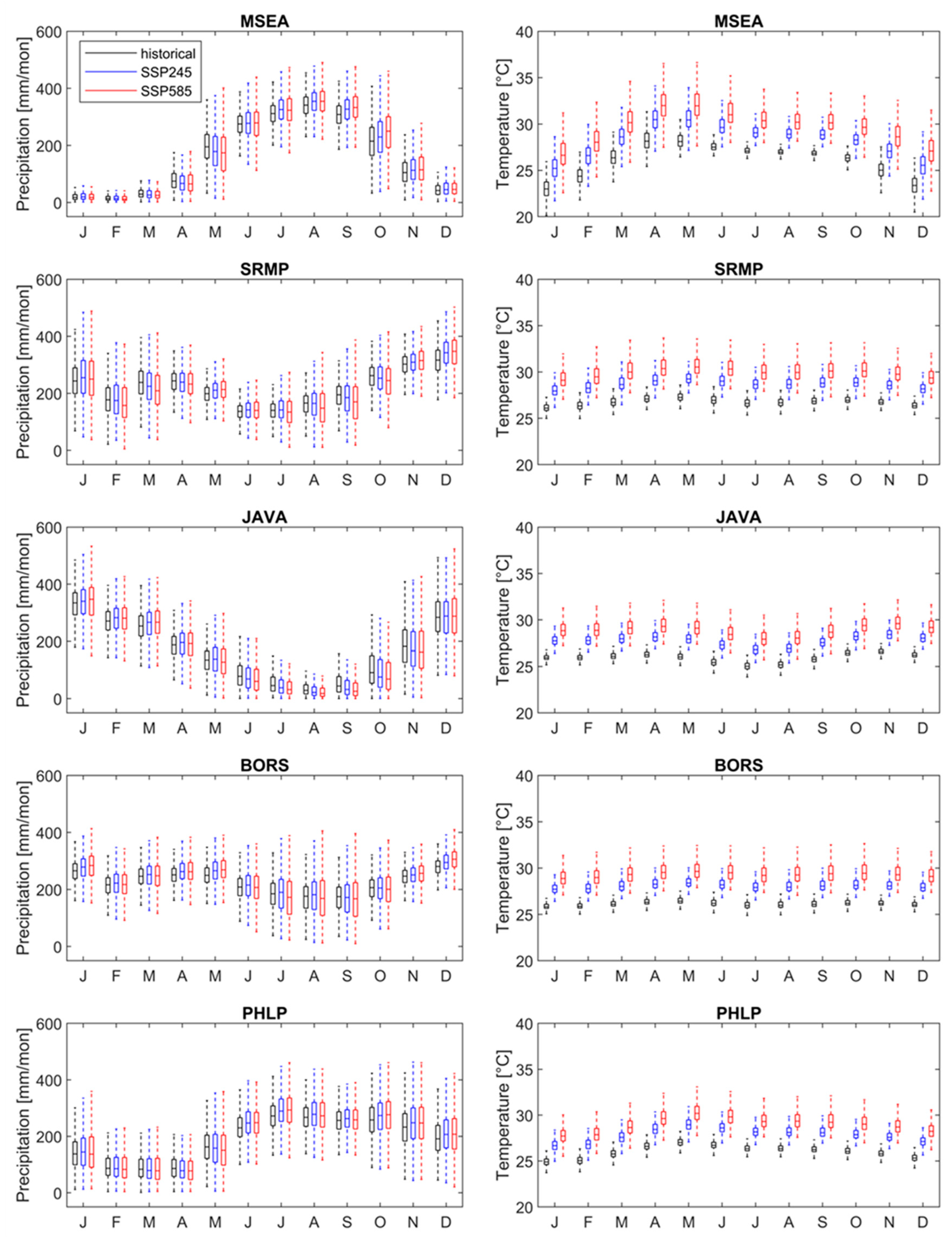
3.3. Seasonal Changes

We have conducted a detailed examination of seasonal variations in precipitation and temperature across the five primary regions in SEA. Figure 5 provides a comprehensive depiction of monthly precipitation and temperature variations in the short-term future (2061–2100) relative to those in the historical period (1950–2014). In the MSEA region, precipitation is suggested to drop by 5.26 to 9.43% for SSP245 and 9.04 to 10.89% for SSP585 during the tail end of the dry season and the onset of the rainy one, specifically from March to May. However, an increase in precipitation is anticipated during the late rainy season, with an uptick of 6.04 to 8.96% (SSP245) and 8.86 to 15.04% (SSP585) observed between September and November. Remarkably, a decline in monthly precipitation is found during the late southwest monsoon (August to October) in the SRMP region, with a range of 0.45 to 5.04% (SSP245) and 5.99 to 11.04 (SSP585). This is followed by an increase in the early northeast monsoon (November to December), with an approximate rise of 3.12 to 8.20% for SSP245 and 4.65 to 9.31% for SSP585.
In the JAVA region, substantial reductions in seasonal rainfall are forecasted during the dry season, spanning from July to October. These reductions are estimated to be in the range of 11.70 to 15.70% for SSP245 and 15.29 to 23.44% for SSP585. Conversely, a modest increase in rainfall is anticipated during the rainy season, with expected increments of 1.60 to 3.05% for SSP245 and 1.80 to 4.93% for SSP585. In the BORS region, the projected average monthly precipitation appears to be evenly distributed throughout the year under both SSP245 and SSP585. Moving on to the PHLP region, a rise in rainfall is projected to occur in the rainy season extending from June to November, with projected increases ranging from 2.60 to 7.32% and 1.02 to 7.72 for the two scenarios, respectively. Conversely, during the dry season (from December to May), changes in rainfall are anticipated to be between −5.58 to 7.43% and −7.99 to 7.42% for SSP245 and SSP585, respectively. In terms of temperature, there is a consistent degree of increase with slight seasonal and monthly variations, but a notable distinction exists between SSP245 and SSP585 scenarios. Specifically, under SSP245, the projected temperature increase is as follows: 2.06 ± 0.12 °C for MSEA, 1.90 ± 0.08 °C for SRMP, 1.82 ± 0.04 °C for JAVA, 1.91 ± 0.04 °C for BORS, and 1.81 ± 0.05 °C for PHLP. Conversely, the SSP585 scenario indicates a higher temperature increase, with values of 3.58 ± 0.19 °C, 3.23 ± 0.12 °C, 3.02 ± 0.06 °C, 3.22 ± 0.09 °C, and 3.02±0.10°C for MSEA, SRMP, JAVA, BORS, and PHLP, respectively.

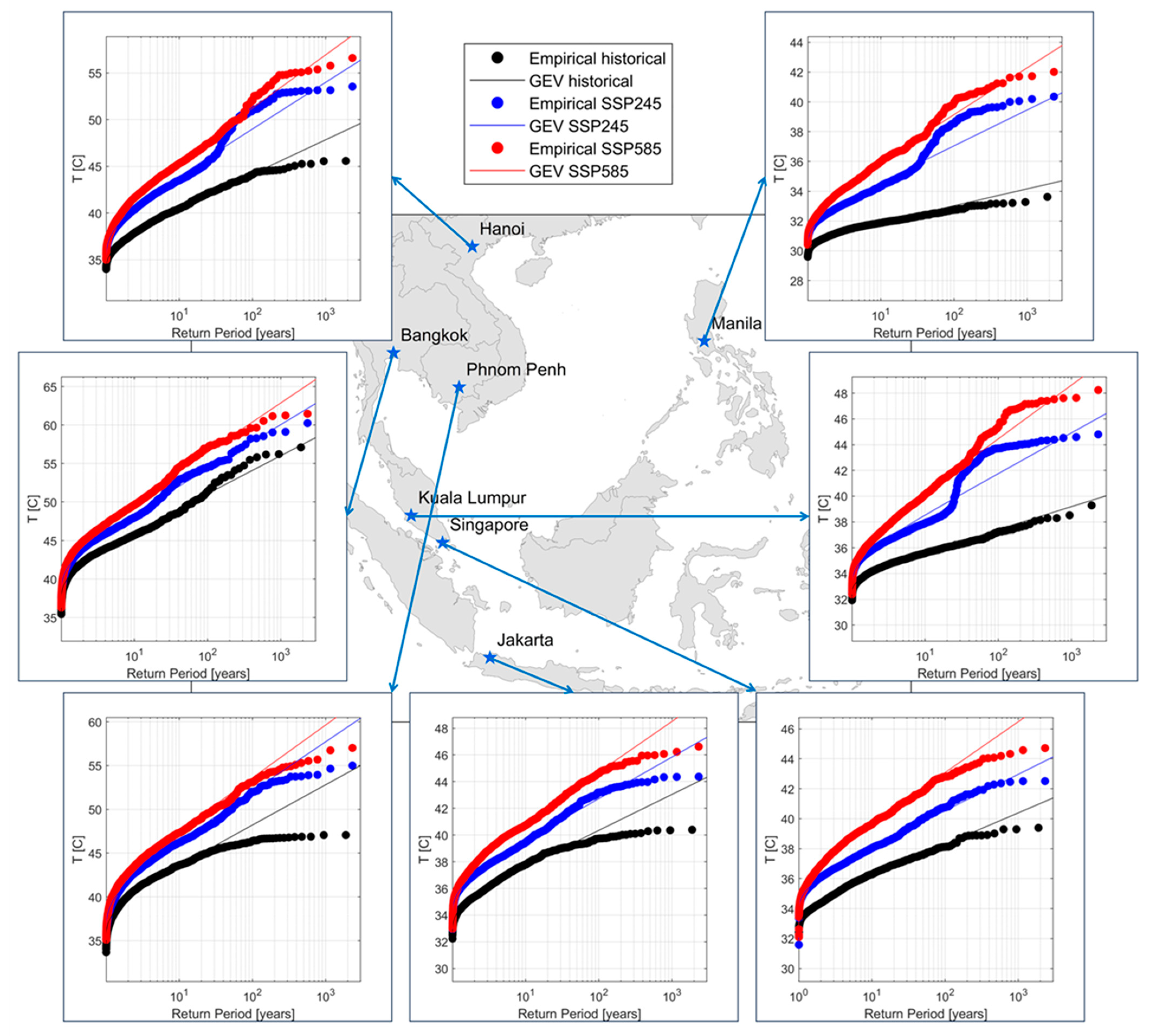
3.4. Localization Outlooks

Figure 6 and Figure 7 visually depict the related AMS results for SEA cities, including Bangkok, Hanoi, Jakarta, Kuala Lumpur, Manila, Phnom Penh, and Singapore. The results consistently indicate that all seven cities demonstrate a rise in intense precipitation in both future projection scenarios (Figure 6). Among these cities, six (excluding Manila) are projected to experience a similarly significant rise in the magnitude of extreme precipitation under various return periods. Specifically, these increases range from 11 to 17%, 18 to 25%, 20 to 31%, and 21 to 33% for the SSP245 scenario, and 22 to 38%, 14 to 21%, 23 to 30%, and 24 to 35% for SSP585 scenario (Table 3). However, Manila exhibits a comparatively lower increase, with a range of 8 to 9% for the SSP245 scenario and 10 to 14% for the SSP585 scenario across return periods from 2 to 100 years.
As Figure 7 clearly illustrates, there is a significant uptick in daily maximum temperature projected for all seven cities in the future under both emission scenarios in contrast to the benchmark of history. Under the SSP245 scenario, extreme temperature is expected to increase similarly across all seven cities in the SEA. These increases are projected to be in the range of 1.04 to 1.06 °C, 1.05 to 1.09 °C, 1.06 to 1.11 °C, and 1.06 to 1.12 °C for all concerned return periods, respectively. In the case of the SSP585 scenario, a more pronounced increase in extreme temperature is foreseen, with ranges of 1.07 to 1.15 °C, 1.06 to 1.13 °C, 1.08 to 1.17 °C, and 1.10 to 1.19 °C projected for the same range of return periods.

4. Discussion and Conclusions

The comprehensive analysis of climate projections for the SEA region, encompassing changes in precipitation and temperature, offers a detailed insight into how climate conditions are expected to evolve in response to the impending climate change impacts. This research has scrutinized these changes in the context of the five main regions within SEA, explored their seasonal variations, and provided localized insights for major cities. The findings are of great significance, bearing profound implications for the region’s future climate and adaptation strategies. In our examination of precipitation changes, we have identified an upward trend in extreme precipitation events across all four indices (RX1day, R20, R99P, and CDD) for both the short-term (2021–2060) and long-term (2061–2100) future under SSP245 and SSP585 scenarios. This suggests that the SEA region can anticipate increasingly frequent and intense rain occurrences in the coming decades, which, in turn, may heighten flood risks and vulnerabilities in social infrastructure, and pose challenges for agriculture and water resources management. It is noteworthy to mention that while this trend is nonuniform across SEA, statistical significance is observed in nearly all extreme precipitation indices and projected periods, affirming the reliability of these findings. Additionally, it is important to note that the analysis of changing increments is based on modeled historical data rather than actual historical data to ensure greater consistency in trend analysis.
Our temperature projections reveal a significant and consistent increase in temperatures across varying time scales and regions. The SSP245 and SSP585 scenarios underscore the pivotal role of reducing greenhouse gas emissions to mitigate future global warming. These temperature increases would bring about a broad spectrum of effects, including heightened heat-related stress, increased energy demand for cooling, shifts in ecosystems, and alterations in agricultural practices [69]. These challenges pose significant difficulties for humanity and society as a whole. The analysis of seasonal changes in precipitation and temperature enhances our understanding of temporal variations. Shifts in rainfall patterns, with some areas experiencing drier dry seasons and wetter rainy seasons, have notable implications for water resources management, agriculture, and ecosystems. Moreover, the localized outlook for major SEA cities highlights the urban challenges posed by increasing extreme storm occurrences, which could bring about a higher risk of urban flooding. Concurrently, rising temperatures can exacerbate heat waves and strain cooling infrastructure, compounding the challenges faced by these urban centers.
The study has identified certain limitations that warrant consideration. It projected future climate extremes in SEA cities utilizing downscaled CMIP6 GCMs with a spatial resolution of approximately 25km. However, this resolution might still lack the necessary granularity to provide detailed insights into specific locations, such as sub-regions within cities. To address this limitation in future research, it is advisable to explore the adoption of a finer spatial resolution. Moreover, the study operated on a daily temporal scale. To enhance the analysis of climate extremes, future studies could benefit from utilizing a higher temporal resolution, such as sub-daily or hourly data. This finer time scale would offer the opportunity for a more detailed examination of rapid changes in extreme weather events, which are becoming increasingly pertinent due to climate change. Furthermore, while the NEX-GDDP-CMIP6 dataset has undergone bias correction against finer resolutions and various statistical characteristics across a large spatial domain, its validity and accuracy require careful evaluation for use in studies at smaller spatial scales [62]. Additional bias correction may be necessary to ensure the local representativeness of the data.
While rainfall data are commonly employed to represent flood hazards, it is vital to recognize that future research should consider incorporating hydrodynamic simulations into their methodologies. The study significantly enhances hydrodynamic modeling and flood risk mitigation by providing high-resolution data through downscaled climate projections. This detailed information allows for more accurate simulations of flood events, as hydrodynamic models can better capture local topography, land use, and hydrological responses to extreme weather. By integrating precise precipitation and temperature data, these models can predict flood extents and durations with greater reliability. Understanding shifts in precipitation and temperature patterns is crucial for assessing flood risks and designing effective drainage systems. The study’s analysis of seasonal changes helps identify areas that may experience wetter rainy seasons, enabling urban planners and engineers to prepare for increased runoff during peak periods. This knowledge is essential for developing infrastructure that can withstand the impacts of extreme weather events.
The findings of the study can inform urban planning efforts by highlighting areas at higher risk of flooding. This information is vital for developing resilient infrastructure, such as green roofs, permeable pavements, and improved drainage systems. Additionally, the study can guide zoning regulations to prevent construction in flood-prone areas, ultimately reducing vulnerability to flooding in urban environments. By identifying potential flooding hotspots and the expected frequency of extreme weather events, the study enables local governments and communities to develop better preparedness plans. This includes establishing early warning systems, community education programs, and emergency response strategies tailored to the specific risks identified. Enhanced community preparedness is essential for minimizing the impacts of flooding on residents and infrastructure.
In conclusion, future research recommendations suggest incorporating land use and economic conditions into analyses, which can help identify vulnerable populations and critical infrastructure that need protection. This holistic approach ensures that mitigation strategies are equitable and effective, addressing the needs of all community members and enhancing overall resilience to flooding. The evidence presented in the study regarding the increasing risks associated with climate change can guide policymakers in developing effective climate adaptation strategies. By highlighting the urgency of addressing these risks, the study supports the formulation of policies aimed at reducing vulnerability and enhancing community resilience against flooding, ultimately contributing to a more sustainable and secure future for affected regions.

Supplementary Materials

The following supporting information can be downloaded at: https://www.mdpi.com/article/10.3390/w16152207/s1. Table S1: List of datasets used in this study; Table S2: List of extreme indicators used in this research [4]; Table S3: List of 29 GCMs for future projection in this study [63].

Author Contributions

Conceptualization, S.T. and X.Q.; methodology, S.T. and X.Q.; software, S.T.; validation, S.T. and X.Q.; formal analysis, S.T.; investigation, S.T.; resources, S.T.; data curation, S.T.; writing—original draft preparation, S.T.; writing—review and editing, X.Q.; visualization, S.T.; supervision, X.Q.; project administration, X.Q.; funding acquisition, X.Q. All authors have read and agreed to the published version of the manuscript.

Funding

This research was funded by Ministry of Education, Singapore, under its MOE Academic Research Fund Tier 1 grant number RG72/22 and in part by the Ministry of Education, Singapore, under its MOE Academic Research Fund Tier 3 grant number MOE-MOET32022-0006.

Data Availability Statement

The climate dataset is freely accessible from NEX-GDDP-CMIP6 at https://nex-gddp-cmip6.s3.us-west-2.amazonaws.com/index.html. The observed hydrological data may be available from the corresponding authors upon reasonable request.

Acknowledgments

This research is supported by the Ministry of Education, Singapore, under its MOE Academic Research Fund Tier 1 (Grant No. RG72/22). This research is also supported in part by the Ministry of Education, Singapore, under its MOE Academic Research Fund Tier 3, Award number MOE-MOET32022-0006. Any opinions, findings, conclusions, or recommendations expressed in this material are those of the authors and do not reflect the views of the Ministry of Education, Singapore. Climate scenarios used were from the NEX-GDDP-CMIP6 dataset, prepared by the Climate Analytics Group and NASA Ames Research Center using the NASA Earth Exchange and distributed by the NASA Center for Climate Simulation (NCCS).

Conflicts of Interest

The authors declare no conflict of interest.

References

  1. Adeyeri, O.E.; Zhou, W.; Wang, X.; Zhang, R.; Laux, P.; Ishola, K.A.; Usman, M. The trend and spatial spread of multisectoral climate extremes in CMIP6 models. Sci. Rep. 2022, 12, 21000. [Google Scholar] [CrossRef] [PubMed]
  2. Chhin, R.; Oeurng, C.; Yoden, S. Drought projection in the Indochina Region based on the optimal ensemble subset of CMIP5 models. Clim. Chang. 2020, 162, 687–705. [Google Scholar] [CrossRef]
  3. Iqbal, Z.; Shahid, S.; Ahmed, K.; Ismail, T.; Ziarh, G.F.; Chung, E.-S.; Wang, X. Evaluation of CMIP6 GCM rainfall in mainland Southeast Asia. Atmos. Res. 2021, 254, 105525. [Google Scholar] [CrossRef]
  4. Thrasher, B.; Wang, W.; Michaelis, A.; Melton, F.; Lee, T.; Nemani, R. NASA global daily downscaled projections, CMIP6. Sci. Data 2022, 9, 262. [Google Scholar] [CrossRef] [PubMed]
  5. Try, S.; Sayama, T.; Phy, S.R.; Sok, T.; Ly, S.; Oeurng, C. Assessing the impacts of climate change and dam development on potential flood hazard and damages in the Cambodian floodplain of the lower mekong basin. J. Hydrol. Reg. Stud. 2023, 49, 101508. [Google Scholar] [CrossRef]
  6. Bourdeau-Goulet, S.; Hassanzadeh, E. Comparisons between CMIP5 and CMIP6 models: Simulations of climate indices influencing food security, infrastructure resilience, and human health in Canada. Earth’s Future 2021, 9, e2021EF001995. [Google Scholar] [CrossRef]
  7. Chen, H.; Sun, J.; Lin, W.; Xu, H. Comparison of CMIP6 and CMIP5 models in simulating climate extremes. Sci. Bull. 2020, 65, 1415–1418. [Google Scholar] [CrossRef] [PubMed]
  8. Seneviratne, S.I.; Hauser, M. Regional climate sensitivity of climate extremes in CMIP6 versus CMIP5 multimodel ensembles. Earth’s Future 2020, 8, e2019EF001474. [Google Scholar] [CrossRef]
  9. Try, S.; Tanaka, S.; Tanaka, K.; Sayama, T.; Khujanazarov, T.; Oeurng, C. Comparison of CMIP5 and CMIP6 GCM performance for flood projections in the Mekong River Basin. J. Hydrol. Reg. Stud. 2022, 40, 101035. [Google Scholar] [CrossRef]
  10. Murphy, J.M.; Sexton, D.M.; Barnett, D.N.; Jones, G.S.; Webb, M.J.; Collins, M.; Stainforth, D.A. Quantification of modelling uncertainties in a large ensemble of climate change simulations. Nature 2004, 430, 768–772. [Google Scholar] [CrossRef]
  11. Chhin, R.; Yoden, S. Ranking CMIP5 GCMs for model ensemble selection on regional scale: Case study of the Indochina Region. J. Geophys. Res. Atmos. 2018, 123, 8949–8974. [Google Scholar] [CrossRef]
  12. Desmet, Q.; Ngo-Duc, T. A novel method for ranking CMIP6 global climate models over the southeast Asian region. Int. J. Climatol. 2022, 42, 97–117. [Google Scholar] [CrossRef]
  13. Ge, F.; Zhu, S.; Luo, H.; Zhi, X.; Wang, H. Future changes in precipitation extremes over Southeast Asia: Insights from CMIP6 multi-model ensemble. Environ. Res. Lett. 2021, 16, 024013. [Google Scholar] [CrossRef]
  14. Le, P.V.; Randerson, J.T.; Willett, R.; Wright, S.; Smyth, P.; Guilloteau, C.; Mamalakis, A.; Foufoula-Georgiou, E. Climate-driven changes in the predictability of seasonal precipitation. Nat. Commun. 2023, 14, 3822. [Google Scholar] [CrossRef] [PubMed]
  15. Peng, S.; Wang, C.; Li, Z.; Mihara, K.; Kuramochi, K.; Toma, Y.; Hatano, R. Climate change multi-model projections in CMIP6 scenarios in Central Hokkaido, Japan. Sci. Rep. 2023, 13, 230. [Google Scholar] [CrossRef] [PubMed]
  16. Rettie, F.M.; Gayler, S.; Weber, T.K.; Tesfaye, K.; Streck, T. High-resolution CMIP6 climate projections for Ethiopia using the gridded statistical downscaling method. Sci. Data 2023, 10, 442. [Google Scholar] [CrossRef] [PubMed]
  17. Rummukainen, M. State-of-the-art with regional climate models. Wiley Interdiscip. Rev. Clim. Change 2010, 1, 82–96. [Google Scholar] [CrossRef]
  18. Giorgi, F.; Francisco, R. Evaluating uncertainties in the prediction of regional climate change. Geophys. Res. Lett. 2000, 27, 1295–1298. [Google Scholar] [CrossRef]
  19. Supharatid, S.; Nafung, J.; Aribarg, T. Projected changes in temperature and precipitation over mainland Southeast Asia by CMIP6 models. J. Water Clim. Change 2022, 13, 337–356. [Google Scholar] [CrossRef]
  20. Ge, F.; Zhi, X.; Babar, Z.A.; Tang, W.; Chen, P. Interannual variability of summer monsoon precipitation over the Indochina Peninsula in association with ENSO. Theor. Appl. Climatol. 2017, 128, 523–531. [Google Scholar] [CrossRef]
  21. Takahashi, H.G.; Yasunari, T. Decreasing trend in rainfall over Indochina during the late summer monsoon: Impact of tropical cyclones. J. Meteorol. Soc. Japan. Ser. II 2008, 86, 429–438. [Google Scholar] [CrossRef]
  22. Wang, B.; Wu, R.; Lau, K. Interannual variability of the Asian summer monsoon: Contrasts between the Indian and the western North Pacific–East Asian monsoons. J. Clim. 2001, 14, 4073–4090. [Google Scholar] [CrossRef]
  23. Faostat, F. Statistical Database; Food and Agriculture Organization of the United Nations: Rome, Italy, 2017. [Google Scholar]
  24. Qin, X.; Dai, C. Comparison of different quantile delta mapping schemes in frequency analysis of precipitation extremes over mainland Southeast Asia under climate change. J. Hydrol. 2022, 606, 127421. [Google Scholar] [CrossRef]
  25. Skliris, N.; Marsh, R.; Haigh, I.D.; Wood, M.; Hirschi, J.; Darby, S.; Quynh, N.P.; Hung, N.N. Drivers of rainfall trends in and around Mainland Southeast Asia. Front. Clim. 2022, 4, 926568. [Google Scholar] [CrossRef]
  26. Endo, N.; Matsumoto, J.; Lwin, T. Trends in precipitation extremes over Southeast Asia. Sola 2009, 5, 168–171. [Google Scholar] [CrossRef]
  27. Hariadi, M.H.; van der Schrier, G.; Steeneveld, G.; Ratri, D.N.; Sopaheluwakan, A.; Tank, A.K.; Aldrian, E.; Gunawan, D.; Moine, M.; Bellucci, A. Evaluation of extreme precipitation over Southeast Asia in the Coupled Model Intercomparison Project Phase 5 regional climate model results and HighResMIP global climate models. Int. J. Climatol. 2023, 43, 1639–1659. [Google Scholar] [CrossRef]
  28. Mandapaka, P.V.; Lo, E.Y. Assessment of future changes in Southeast Asian precipitation using the NASA Earth Exchange Global Daily Downscaled Projections data set. Int. J. Climatol. 2018, 38, 5231–5244. [Google Scholar] [CrossRef]
  29. Singh, V.; Qin, X. Study of rainfall variabilities in Southeast Asia using long-term gridded rainfall and its substantiation through global climate indices. J. Hydrol. 2020, 585, 124320. [Google Scholar] [CrossRef]
  30. Tangang, F.; Juneng, L.; Cruz, F.; Chung, J.X.; Ngai, S.T.; Salimun, E.; Mohd, M.S.F.; Santisirisomboon, J.; Singhruck, P.; PhanVan, T. Multi-model projections of precipitation extremes in Southeast Asia based on CORDEX-Southeast Asia simulations. Environ. Res. 2020, 184, 109350. [Google Scholar]
  31. Kim, I.-W.; Oh, J.; Woo, S.; Kripalani, R. Evaluation of precipitation extremes over the Asian domain: Observation and modelling studies. Clim. Dyn. 2019, 52, 1317–1342. [Google Scholar] [CrossRef]
  32. Liu, S.; Raghavan, S.V.; Ona, B.J.; Nguyen, N.S. Bias evaluation in rainfall over Southeast Asia in CMIP6 models. J. Hydrol. 2023, 621, 129593. [Google Scholar] [CrossRef]
  33. Ly, S.; Sayama, T.; Try, S. Integrated impact assessment of climate change and hydropower operation on streamflow and inundation in the lower Mekong Basin. Prog. Earth Planet. Sci. 2023, 10, 55. [Google Scholar] [CrossRef]
  34. Thanvisitthpon, N.; Shrestha, S.; Pal, I. Urban flooding and climate change: A case study of Bangkok, Thailand. Environ. Urban. ASIA 2018, 9, 86–100. [Google Scholar] [CrossRef]
  35. Worawiwat, A.; Chaleeraktrakoon, C.; Sharma, A. Is Increased Flooding Bangk. A Result Rising Local Temp? J. Hydrol. X 2021, 13, 100095. [Google Scholar]
  36. Duy, P.; Chapman, L.; Tight, M.; Thuong, L.; Linh, P. Urban resilience to floods in coastal cities: Challenges and opportunities for Ho Chi Minh city and other emerging cities in southeast Asia. J. Urban Plan. Dev. 2018, 144, 05017018. [Google Scholar] [CrossRef]
  37. Luo, P.; Mu, D.; Xue, H.; Ngo-Duc, T.; Dang-Dinh, K.; Takara, K.; Nover, D.; Schladow, G. Flood inundation assessment for the Hanoi Central Area, Vietnam under historical and extreme rainfall conditions. Sci. Rep. 2018, 8, 12623. [Google Scholar] [CrossRef]
  38. Heng, S.; Ly, S.; Chhem, S.; Kruy, P. Analysis of Public Perceptions on Urban Flood in Phnom Penh, Cambodia. In Water Security in Asia: Opportunities and Challenges in the Context of Climate Change; Springer: Berlin/Heidelberg, Germany, 2021; pp. 687–701. [Google Scholar]
  39. Thuon, T.; Cai, Y. Resistance for resilience: A reflexive exploration of battambang, Cambodia. In Urban Climate Resilience in Southeast Asia; Springer: Cham, Swizerland, 2019; pp. 127–146. [Google Scholar]
  40. Reeder, G. Urban Governance of flooding in Myanmar: A case study of bago. In Urban Climate Resilience in Southeast Asia; Springer: Cham, Swizerland, 2019; pp. 103–126. [Google Scholar]
  41. Zin, W.W.; Kawasaki, A.; Takeuchi, W.; San, Z.M.L.T.; Htun, K.Z.; Aye, T.H.; Win, S. Flood hazard assessment of Bago river basin, Myanmar. J. Disaster Res. 2018, 13, 14–21. [Google Scholar] [CrossRef]
  42. Phanuwan, C.; Takizawa, S.; Oguma, K.; Katayama, H.; Yunika, A.; Ohgaki, S. Monitoring of human enteric viruses and coliform bacteria in waters after urban flood in Jakarta, Indonesia. Water Sci. Technol. 2006, 54, 203–210. [Google Scholar] [CrossRef] [PubMed]
  43. Rendana, M.; Mohd Razi Idris, W.; Abdul Rahim, S.; Abdo, H.G.; Almohamad, H.; Abdullah Al Dughairi, A. Flood risk and shelter suitability mapping using geospatial technique for sustainable urban flood management: A case study in Palembang city, South Sumatera, Indonesia. Geol. Ecol. Landsc. 2023, 1–11. [Google Scholar] [CrossRef]
  44. Garcia, F.C.C.; Retamar, A.E.; Javier, J.C. A real time urban flood monitoring system for metro Manila. In Proceedings of the TENCON 2015–2015 IEEE Region 10 Conference, Macao, China, 1–4 November 2015; pp. 1–5. [Google Scholar]
  45. Zoleta-Nantes, D.B. Flood hazards in Metro Manila: Recognizing commonalities, differences, and courses of action. Soc. Sci. Diliman 2007, 1, 60–105. [Google Scholar]
  46. Sayama, T.; Tatebe, Y.; Iwami, Y.; Tanaka, S. Hydrologic sensitivity of flood runoff and inundation: 2011 Thailand floods in the Chao Phraya River basin. Nat. Hazards Earth Syst. Sci. 2015, 15, 1617–1630. [Google Scholar] [CrossRef]
  47. MRC. Annual Mekong Flood Report 2011. Mekong River Commission, Vientiane, Lao PDR. 2015. Available online: https://reliefweb.int/report/cambodia/annual-mekong-flood-report-2011 (accessed on 25 May 2023).
  48. Budiyono, Y.; Aerts, J.C.; Tollenaar, D.; Ward, P.J. River flood risk in Jakarta under scenarios of future change. Nat. Hazards Earth Syst. Sci. 2016, 16, 757–774. [Google Scholar] [CrossRef]
  49. Lagmay, A.M.; Mendoza, J.; Cipriano, F.; Delmendo, P.A.; Lacsamana, M.N.; Moises, M.A.; Pellejera, N., III; Punay, K.N.; Sabio, G.; Santos, L. Street floods in Metro Manila and possible solutions. J. Environ. Sci. 2017, 59, 39–47. [Google Scholar] [CrossRef] [PubMed]
  50. Dutta, D. An integrated tool for assessment of flood vulnerability of coastal cities to sea-level rise and potential socio-economic impacts: A case study in Bangkok, Thailand. Hydrol. Sci. J. 2011, 56, 805–823. [Google Scholar] [CrossRef]
  51. Bhuiyan, T.R.; Reza, M.I.H.; Choy, E.A.; Pereira, J.J. Facts and trends of urban exposure to flash flood: A case of Kuala Lumpur City. In Improving Flood Management, Prediction and Monitoring; Emerald Publishing Limited: Bingley, UK, 2018; pp. 79–90. [Google Scholar]
  52. Vachaud, G.; Quertamp, F.; Phan, T.S.H.; Ngoc, T.D.T.; Nguyen, T.; Luu, X.L.; Nguyen, A.T.; Gratiot, N. Flood-related risks in Ho Chi Minh City and ways of mitigation. J. Hydrol. 2019, 573, 1021–1027. [Google Scholar] [CrossRef]
  53. Yatagai, A.; Kamiguchi, K.; Arakawa, O.; Hamada, A.; Yasutomi, N.; Kitoh, A. APHRODITE: Constructing a long-term daily gridded precipitation dataset for Asia based on a dense network of rain gauges. Bull. Am. Meteorol. Soc. 2012, 93, 1401–1415. [Google Scholar] [CrossRef]
  54. Noor, M.; Ismail, T.; Shahid, S.; Nashwan, M.S.; Ullah, S. Development of multi-model ensemble for projection of extreme rainfall events in Peninsular Malaysia. Hydrol. Res. 2019, 50, 1772–1788. [Google Scholar] [CrossRef]
  55. Sunilkumar, K.; Yatagai, A.; Masuda, M. Preliminary evaluation of GPM-IMERG rainfall estimates over three distinct climate zones with APHRODITE. Earth Space Sci. 2019, 6, 1321–1335. [Google Scholar] [CrossRef]
  56. Try, S.; Tanaka, S.; Tanaka, K.; Sayama, T.; Oeurng, C.; Uk, S.; Takara, K.; Hu, M.; Han, D. Comparison of gridded precipitation datasets for rainfall-runoff and inundation modeling in the Mekong River Basin. PLoS ONE 2020, 15, e0226814. [Google Scholar] [CrossRef]
  57. Chen, M.; Shi, W.; Xie, P.; Silva, V.B.; Kousky, V.E.; Wayne Higgins, R.; Janowiak, J.E. Assessing objective techniques for gauge-based analyses of global daily precipitation. J. Geophys. Res. Atmos. 2008, 113, D04110. [Google Scholar] [CrossRef]
  58. Haile, A.T.; Habib, E.; Rientjes, T. Evaluation of the climate prediction center (CPC) morphing technique (CMORPH) rainfall product on hourly time scales over the source of the Blue Nile River. Hydrol. Process. 2013, 27, 1829–1839. [Google Scholar] [CrossRef]
  59. McKinnon, K.A.; Rhines, A.; Tingley, M.; Huybers, P. Long-lead predictions of eastern United States hot days from Pacific sea surface temperatures. Nat. Geosci. 2016, 9, 389–394. [Google Scholar] [CrossRef]
  60. Sun, Q.; Miao, C.; Duan, Q.; Ashouri, H.; Sorooshian, S.; Hsu, K. A review of global precipitation data sets: Data sources, estimation, and intercomparisons. Rev. Geophys. 2018, 56, 79–107. [Google Scholar] [CrossRef]
  61. Wood, A.W.; Leung, L.R.; Sridhar, V.; Lettenmaier, D.P. Hydrologic implications of dynamical and statistical approaches to downscaling climate model outputs. Clim. Change 2004, 62, 189–216. [Google Scholar] [CrossRef]
  62. Thrasher, B.; Maurer, E.P.; McKellar, C.; Duffy, P.B. Technical Note: Bias correcting climate model simulated daily temperature extremes with quantile mapping. Hydrol. Earth Syst. Sci. 2012, 16, 3309–3314. [Google Scholar] [CrossRef]
  63. Zhang, X.; Alexander, L.; Hegerl, G.C.; Jones, P.; Tank, A.K.; Peterson, T.C.; Trewin, B.; Zwiers, F.W. Indices for monitoring changes in extremes based on daily temperature and precipitation data. Wiley Interdiscip. Rev. Clim. Change 2011, 2, 851–870. [Google Scholar] [CrossRef]
  64. Massey, F.J., Jr. The Kolmogorov-Smirnov test for goodness of fit. J. Am. Stat. Assoc. 1951, 46, 68–78. [Google Scholar] [CrossRef]
  65. Singh, V.P.; Singh, V.P. Generalized extreme value distribution. In Entropy-Based Parameter Estimation in Hydrology; Springer Nature: Dordrecht, The Netherlands, 1998; pp. 169–183. [Google Scholar]
  66. Demirel, M.C.; Mai, J.; Mendiguren, G.; Koch, J.; Samaniego, L.; Stisen, S. Combining satellite data and appropriate objective functions for improved spatial pattern performance of a distributed hydrologic model. Hydrol. Earth Syst. Sci. 2018, 22, 1299–1315. [Google Scholar] [CrossRef]
  67. Pearson, K. Early Statistical Papers; Cambridge University Press: Cambridge, UK, 1948; pp. 1–40. [Google Scholar]
  68. Roberts, N.M.; Lean, H.W. Scale-selective verification of rainfall accumulations from high-resolution forecasts of convective events. Mon. Weather. Rev. 2008, 136, 78–97. [Google Scholar] [CrossRef]
  69. Wu, Y.H.; Huang, C.Z.; Huang, W.W.; Chen, X.J. Projected changes in temperature and precipitation over Canada in the 21st Century. J. Environ. Inform. 2024. [Google Scholar] [CrossRef]
Figure 1. Study area of Southeast Asia: (a) five geographical masks for regional analysis including Mainland Southeast Asia (MSEA), Sumatra and Malay Peninsula (SRMP), Java Island (JAVA), Borneo and Sulawesi Islands (BORS), and the Philippines (PHLP); and (b) digital elevation map for the study region. The country administrative boundaries were accessed from open data provided by the World Food Programme (a UN agency) at https://public.opendatasoft.com/explore/dataset/world-administrative-boundaries (accessed on 30 May 2023). The digital elevation data was freely available from HydroSHEDS at https://www.hydrosheds.org/hydrosheds-core-downloads (accessed on 30 May 2023).
Water 16 02207 g001
Figure 2. Comparison of precipitation indices from APHRODITE with historical NEX-GDDP-CMIP6 dataset. The bias was calculated by using the NEX-GDDP-CMIP6 dataset subtracted from the APHRODITE dataset.
Water 16 02207 g002
Figure 3. Comparison of temperature indices from CPC with historical NEX-GDDP-CMIP6 dataset. The bias was calculated by using the NEX-GDDP-CMIP6 dataset subtracted from the CPC dataset.
Water 16 02207 g003
Figure 4. Comparison of precipitation (a,b) and temperature changes (c,d) from the future projection period (2021–2085) compared to the baseline period (1950–2014). The hatch fills represent the significance of K-S test at a significant level of 1%.
Water 16 02207 g004
Figure 5. Monthly changes in precipitation (left column) and temperature (right column) over the five main regions in SEA in the far future (2061–2100) compared to the baseline period (1950–2014).
Water 16 02207 g005
Figure 6. Changes in extreme and frequency of precipitation in SEA cities. The dots and lines represent the empirical and GEV fitting for the future projections under the SSP245 (blue) and SSP585 (red) scenarios compared to the historical period (black).
Water 16 02207 g006
Figure 7. Changes in extreme and frequency of temperature in SEA cities. The dots and lines represent the empirical and GEV fitting for the future projections under the SSP245 (blue) and SSP585 (red) scenarios compared to the historical period (black).
Water 16 02207 g007
Table 1. Change ratios for precipitation indicators for each region in both the short-term and long-term future periods when compared to the baseline period 1950–2014. (*) and (**) represent statistical significance of K-S test at significant levels 1% and 0.1%.
ScenarioRegionRX1dayR20R99PCDD
Near FutureFar FutureNear FutureFar FutureNear FutureFAR FutureNear FutureFar Future
SSP245MSEA1.10 **1.15 **1.06 **1.13 **1.06 **1.10 **1.02 *1.02 *
SRMP1.12 **1.19 **1.10 **1.21 **1.05 **1.09 **1.14 **1.20 **
JAVA1.07 **1.12 **1.011.07 **1.02 **1.06 **1.14 **1.15 **
BORS1.13 **1.19 **1.17 **1.31 **1.05 **1.09 **1.12 **1.19 **
PHLP1.08 **1.10 **1.08 **1.12 **1.05 **1.08 **1.07 **1.11 **
SSP585MSEA1.12 **1.23 **1.07 **1.20 **1.07 **1.16 **1.021.05 **
SRMP1.13 **1.27 **1.12 **1.31 **1.06 **1.13 **1.18 **1.51 **
JAVA1.08 **1.17 **1.031.11 **1.03 **1.08 **1.13 **1.29 **
BORS1.14 **1.29 **1.20 **1.50 **1.06 **1.14 **1.16 **1.43 **
PHLP1.07 **1.16 **1.07 **1.15 **1.05 **1.12 **1.09 **1.21 **
Table 2. Changes in temperature indicators in degrees Celsius [°C] for each region in the short-term and long-term future periods when compared to the baseline period 1950–2014.
ScenarioRegionTXmaxTmax90PTNminTmin10P
Near FutureFar FutureNear FutureFar FutureNear FutureFar FutureNear FutureFar Future
SSP245MSEA1.502.421.522.480.851.800.911.86
SRMP1.432.291.392.250.951.770.891.68
JAVA1.231.981.231.990.941.650.921.64
BORS1.362.201.342.161.001.790.981.75
PHLP1.272.071.262.040.961.690.931.65
SSP585MSEA1.694.121.784.091.203.441.253.51
SRMP1.643.901.643.801.223.001.132.88
JAVA1.443.261.453.261.152.801.132.76
BORS1.613.741.603.641.253.041.222.98
PHLP1.533.431.513.381.202.811.152.74
Note: All shown numbers in the table are at significant level of 0.1%.
Table 3. Ratio changes in extreme events of precipitation and temperature over seven cities in SEA.
VariableCitySSP245 [Years]SSP585 [Years]
2105010021050100
Precipitation change [%]Bangkok1120252630142530
Hanoi1219222325162428
Jakarta1123303238152735
Kuala Lumpur1723262730213034
Manila899910121414
Phnom Penh1318202122182324
Singapore1425313337162935
Temperature change [°C]Bangkok1.712.382.973.222.683.884.945.39
Hanoi2.423.504.434.843.375.036.477.08
Jakarta1.601.952.252.382.343.244.034.37
Kuala Lumpur1.782.923.924.342.634.606.327.04
Manila1.662.713.634.022.424.075.516.12
Phnom Penh1.912.783.543.852.763.944.975.40
Singapore1.611.892.132.232.403.464.394.78
Disclaimer/Publisher’s Note: The statements, opinions and data contained in all publications are solely those of the individual author(s) and contributor(s) and not of MDPI and/or the editor(s). MDPI and/or the editor(s) disclaim responsibility for any injury to people or property resulting from any ideas, methods, instructions or products referred to in the content.

