Article

An Improved Index-Velocity Method for Calculating Discharge in Meandering Rivers

School of Electronics and Information Engineering, Guangxi Normal University, Guilin 541000, China
*
Author to whom correspondence should be addressed.
Water 2024, 16(17), 2361; https://doi.org/10.3390/w16172361
Submission received: 22 July 2024 / Revised: 14 August 2024 / Accepted: 20 August 2024 / Published: 23 August 2024

Abstract

:
Accurately measuring river flow is not only crucial for hydrologists monitoring hydrological processes but also important for all professionals involved in hydrological research. The ultrahigh frequency (UHF) band enables the surface flow velocity measurement at a deeper effective water depth, so it is less susceptible to the influence of wind drift. However, in curved river channels, the spatial variation in surface velocity is caused by the uneven erosion of the water flow, and this variation is influenced by both air shear stress and the curvature of the river. To mitigate the impact of water level on cross-sectional flow velocity estimation and address the nonlinear relationship between cross-sectional area and water level, this paper proposes a model that is independent of river water level. The nonlinear relationship between cross-sectional area and water level is calculated using a Taylor series expansion. The model was validated using experimental data collected from the Xiantao section of the Han River in Hubei, China, from March to July 2018. The data were discussed separately for high-flow and low-flow periods and were divided into training and validation sets in an 8:2 ratio. Compared to the previous method, our improved method reduces the Root Mean Square Error (RMSE) and Mean Absolute Percentage Error (MAPE) by approximately 2%. In the estimation of flow during the dry season, the improved method achieved a correlation coefficient of 0.9523, representing an increase of 0.1243 compared to the original method. The RMSE was 23.0383, and the MAPE was 0.0232, showing reductions of 23.144 and 0.0241, respectively, compared to the original method. In the estimation of discharge during the wet season, the improved method achieved a correlation coefficient of 0.9908, an increase of 0.0575 compared to the original method. The RMSE was 65.4929, and the MAPE was 0.0391, reflecting reductions of 75.1271 and 0.0338, respectively, compared to the original method. This advancement further enhances the application of UHF radar for discharge measurement in meandering rivers.

1. Introduction

The monitoring of river flow is of great importance for the water cycle, flood prevention, and climate change, making it essential to stay informed about changes in river flow promptly [1,2,3]. With this monitoring approach, we can gain a better understanding of river pollution and conduct timely assessments. In addition, obtaining real-time river flow data during the flood season is crucial for flood control; these data also provide a reference for hydraulic and related engineering projects, which are closely linked to people’s economic lives and navigation [4]. For instance, hydropower generation, port construction, and inland navigation all necessitate relevant hydrological information. Understanding the hydrological data and trends of the associated watershed assist in predicting the interactions between water bodies, climate, and the ecosystem. Therefore, obtaining accurate discharge data requires two key factors: one is precise parameters such as water level and velocity, and the other is using an appropriate discharge inversion algorithm to calculate the flow rate.
The technology and equipment related to water level monitoring have become well-established. The acquisition of river flow data relies on both the monitoring of flow velocity and the application of flow inversion algorithms. The measurement of river flow is mainly divided into two types: contact measurement and non-contact measurement. Contact measurement is more widely used in traditional methods [5], such as mechanical flow meters, Acoustic Doppler Velocimeters (ADV, ADVM), and Acoustic Doppler Current Profilers (ADCP). The mechanical structure and flow measurement principle are relatively simple, but this type of instrument needs to be immersed in water for measurement [6]. Since the instrument is in the water, it may be affected by aquatic plants and animals, leading to reduced measurement accuracy and even posing a risk of instrument damage.
The Acoustic Doppler Velocimeter requires specific installation conditions, making installation and maintenance somewhat challenging. Traditional contact measurement methods, which require direct contact with water, bring about high maintenance costs, environmental impact, and low measurement efficiency. In response to the issues associated with contact measurement, non-contact measurement methods have emerged. For example, remote sensing technology, flow meters, or ultra-high frequency radar can be used for direct or indirect flow measurement [7,8]. Unlike contact measurement, non-contact measurement only measures the surface flow velocity of the river. Remote sensing photography technology, via satellites or drones, can be used to measure the surface flow velocity of rivers, which can then be used to calculate the flow rate based on the surface velocity [9,10]. However, remote sensing measurement of river surface flow velocity is susceptible to weather conditions. When cloud cover is dense, the captured images may be unclear, which can affect the extraction of river flow velocity.
The existing flow velocity inversion algorithms mainly include the index velocity method, semi-empirical and semi-theoretical formulas for obtaining cross-sectional velocity distribution, and velocity distribution derived from fluid dynamics principles [11,12,13]. The semi-empirical and semi-theoretical formulas are primarily applied in non-contact methods for wide and shallow straight river channels. However, for narrow, deep, and curved rivers, some underwater flow velocity data or related parameters are needed [14]. However, the velocity distribution derived from fluid dynamics is mostly based on regular river channels, making it difficult to apply in natural rivers. Existing algorithms can be divided into two categories: one type involves inversion using parameters such as river width, water depth, and water level without considering river flow velocity, while the other, more mainstream approach, uses flow velocity for inversion. The most commonly used methods in the first category of algorithms include the stage–discharge rating curve [15] and the Manning formula. The algorithm that uses water level to invert flow rate requires fitting with long-term water level data and demands a high degree of river stability. The Manning formula has certain limitations in its application, as calculations for natural river channels can be quite complex. The second category of methods mainly includes the five-point method [16], the index velocity method, the exponential method, and the logarithmic method [17]. The five-point method is mostly used in contact measurements, while the index velocity and logarithmic methods fall under semi-empirical, semi-theoretical formulas. These methods often require complex parameters, making them difficult to apply in non-contact measurements. The index velocity method has achieved good results in contact-based river applications. Some researchers have also applied it to non-contact river measurements and have obtained promising results.
Ultra-high frequency radar technology has become increasingly mature and can be used for measuring river flow velocity [17,18,19]. Its measurement principle is based on the Bragg scattering theory and the Doppler effect. After obtaining the surface flow velocity of the river, the flow rate can be calculated using machine learning algorithms [20,21,22,23], the logarithmic method, the velocity–area method [24,25], or the exponential velocity method [26,27]. In recent years, there has been a proposal to use the exponential velocity method for real-time monitoring of river flow [28,29]. The current methods for calculating the average cross-sectional flow velocity of rivers using the exponential velocity method must consider the impact of water level. When water level fluctuations are small, using radar to measure the water level may result in significant errors. Additionally, in curved rivers, the flow velocity distribution on both sides of the riverbed is asymmetrical, which may lead to changes in the main channel of the river and even cause the river to breach its banks [30,31,32,33]. Therefore, it is necessary to monitor changes in the velocity or discharge distribution in curved rivers.
The main contributions of this study can be summarized as follows: (1) The proposed method for calculating river discharge does not rely on water level parameters, reducing the impact of changes in river water level due to varying rainfall on the calculation of river discharge. (2) The proposed method considers the nonlinear relationship between irregular cross-sectional area and water level when calculating river cross-sectional area. (3) The proposed model uses a Taylor series expansion to address the nonlinear relationship between cross-sectional area and water level.
The remainder of this article is organized as follows: Section 2 introduces the proposed method. Section 3 provides the experimental results. Section 4 presents the discussion associated with the proposed method. Section 5 presents a summary of this paper.

2. Method

2.1. Previous Index-Velocity Method

This approach involves calculating river discharge by multiplying the average velocity across a river’s cross-section with the cross-sectional area. The equation used for this calculation is as (1):
Q = V m e a n × A
In the formula, Q represents the river discharge, v m e a n represents the mean velocity across the river cross-section, and A represents the area of the river cross-section. The cross-sectional velocity can be determined using the index-velocity method, which establishes the relationship between the surface and cross-sectional velocities of the river. The model for the index-velocity method is shown in Equation (2) as referenced in [29].
V m e a n = a V i n d H + b V i n d + c
In the formula, v m e a n represents the mean cross-sectional velocity, v i n d represents the index velocity, and a , b , c represents the regression coefficient. As seen from the equation, calculating the mean cross-sectional velocity of a river requires consideration of not only the index velocity but also the impact of water levels.
When UHF radar to measure water level, significant measurement errors can result in calculated discharges that deviate substantially from actual values. Thus, incorporating the variable of water level can introduce errors into the equation, which may amplify during calculations and subsequently affect the accuracy of the estimated river discharge. Therefore, it is necessary to optimize this model to reduce the impact of water level errors on the estimation of mean cross-sectional velocity, thereby improving calculation accuracy and minimizing errors in river discharge estimation.
The cross-sectional area of a river is primarily calculated through approximation methods or by performing sectional integration. For example, for the regular river channel cross-section shown in Figure 1, the cross-sectional area can be calculated using the (3):
A = x 1 x 2 [ h L ( x ) ] d x
In the equation, h represents the height of the riverbed, while x 1 and x 2 represent the upper and lower boundaries of the river surface, respectively. It can be seen from the equation that A is a nonlinear function of h. However, within a very small range of h changes, it can be represented by a linear relationship (4):
A = α h + β
However, for a curved river, the cross-sectional conditions of the river are approximate as shown in Figure 2. The traditional linear model estimation cannot accurately estimate the cross-sectional area. Additionally, due to the influence of the monsoon climate, the range of water level fluctuations increases with the amount of rainfall. Therefore, using Equation (4) to estimate the cross-sectional area of a curved river is not suitable.

2.2. Improved Index-Velocity Method

In response to the above raising issue, the next step is to make a near improvement to the formula for fitting the mean cross-section velocity using the index-velocity method. Equation (5) shows the improved model.
V m e a n = a V 2 i n d + b V i n d + c
The improved model deletes the effect of water level on the calculation of cross-section velocity, and the use of second-order models for fitting the mean cross-section velocity of a river is also very frequent.
The river channel can be eroded into the cross-section shown in Figure 2 due to the uneven scouring by the water flow in meandering rivers. During the flood season, as water levels rise, the rate of change in the water depth D ( x ) at position x is not constant but increases with the rise in h. This paper uses an exponential function to describe the relationship between A and h for such situations. To calculate the cross-sectional area more accurately, a Taylor series can be used within the nonlinear model. According to the mean value theorem of the Taylor series, if a function has derivatives up to the order at some neighborhood of the point a, then within that neighborhood, the n th order Taylor formula for f ( x ) is:
f ( x ) = f ( x 0 ) + L ( x 0 ) ( x x 0 ) + f ( x 0 ) 2 ! ( x x 0 ) 2 + + f n ( x 0 ) n ! ( x x 0 ) ( n ) + R n ( x )
In the formula, R n ( x ) = [ f ( n + 1 ) ( n + 1 ) ! ( x x 0 ) ( n + 1 ) ] represents the Lagrange form of the remainder. To establish a nonlinear relationship between the river cross-section and water level for the meandering river shown in (7).
S ( h ) = S ( h 0 ) + f ( h 0 ) ( h h 0 ) + S ( h 0 ) 2 ! ( h h 0 ) 2 + + S n ( h 0 ) n ! ( h h 0 ) ( n ) + R n ( h )
In the equation, S , S , and S are, respectively, the first, second, and third derivatives of S at h = h 0 . By substituting the expanded forms of S ( h ) into Equation (6), we can approximate the area of the river channel. From Equation (3), we deduce that S is a nonlinear function of h, which allows us to express S as a Taylor series expansion in terms of h. Furthermore, Equation (5) indicates that the cross-sectional flow velocity is independent of h, thus enabling the use of the Taylor series expansion. If the change in h is relatively small, only a few initial terms are needed to achieve a good approximation. Conversely, if the change in h is more significant, more terms need to be considered. Considering the monsoonal climate, which results in periods of high and low water levels in the river, this paper chooses to discuss these periods separately. It is assumed that during these different periods, water level changes are not significant. Therefore, for the Taylor series expansion of the river’s cross-sectional area, only the first three terms are selected for discussion.

2.3. Selection of Index Velocity

The maximum velocity was chosen as the index velocity for straight river channels [29,30]; however, this method is not suitable for curved river channels. In meandering channels, the nearby water surface is affected by air shear stress, resulting in a decrease in the river’s surface velocity as indicated in [31]. The river’s velocity decays more rapidly in areas of higher curvature and more slowly in areas of lesser curvature. Additionally, in meandering channels, the maximum velocity may be influenced by the hydraulic resistance within the river, which also means that the index velocity for this paper’s river cannot be selected as the average maximum velocity as it would be for straight channels. For the context of this paper, averaging the surface velocities to use as the index velocity will to some extent mitigate the impact of meandering channels on the surface velocity.

3. Experiment Analysis

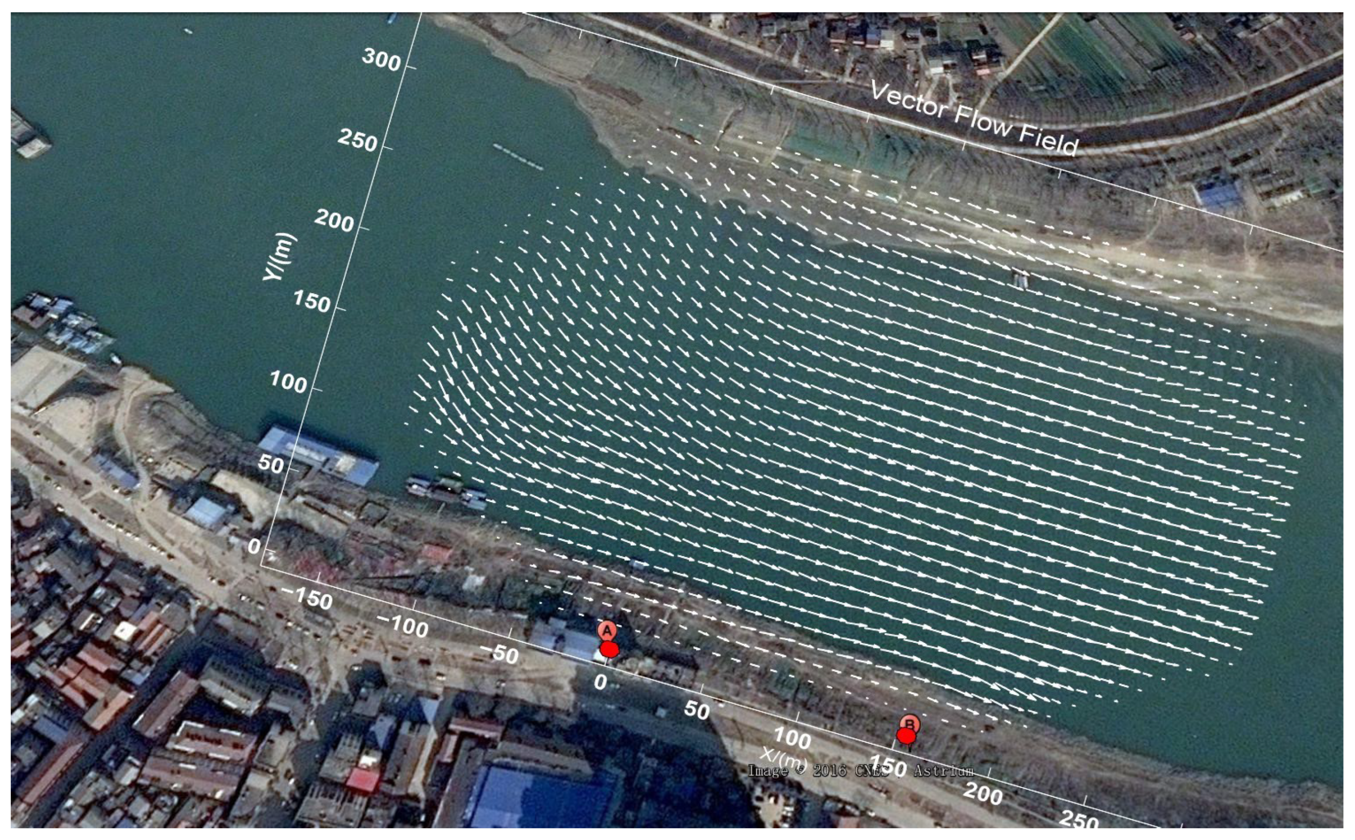
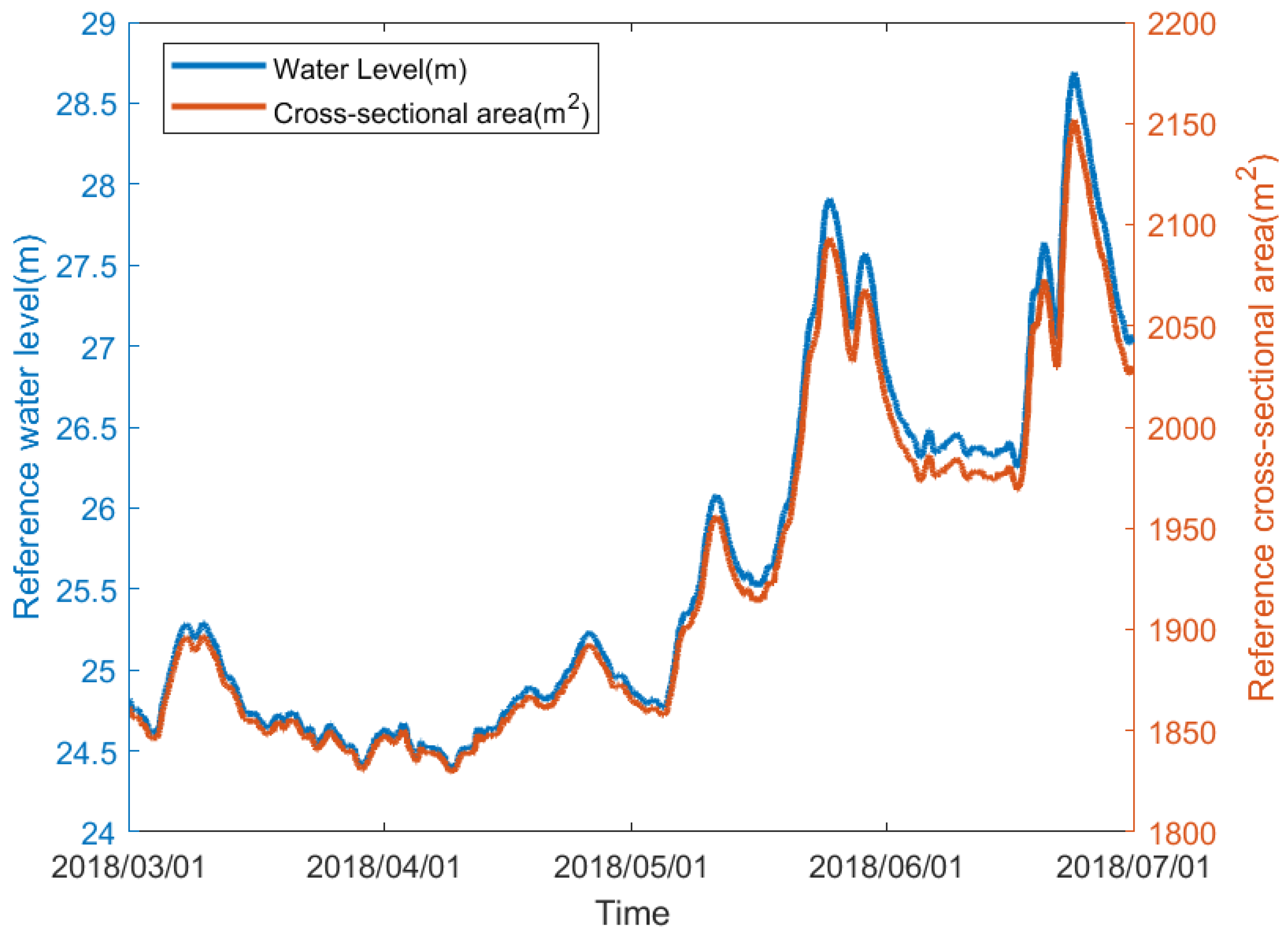
3.1. Experiment Description

To validate the aforementioned method, the experimental data collected by the Ultra High Frequency (UHF) ground wave radar at the Xiantao section of the Han River (113°26′49.62″ E, 30°22′45.76″ N) from March to July 2018, operated by the Radar Signal Processing Laboratory of Wuhan University, was analyzed. The river width at the Xiantao hydrological station ranges from 250 m to 300 m and is located in a curved section of the river, making the flow direction more complex compared to straight river channels. According to historical data, the river flow rate in the Xiantao section of the Han River ranges from 500 to 10,000 cubic meters per second. The UHF radar uses a Frequency Modulated Interrupted Continuous Wave (FMICW) with a carrier frequency of 340 MHz and a bandwidth of 15 MHz, with a coherent accumulation time of 20 s. Two radars are deployed at the Xiantao hydrological station on the Han River, the largest tributary of the Yangtze River. Station A is located inside the hydrological station, with the receiving antenna about 10–15 m above the water surface, and Station B is constructed about 100 m downstream at a height of about 10 m above the water surface. Figure 3 shows the distribution diagram of the dual-station radar, and Figure 4 presents the cross-sectional schematic of the river under study, where the maximum water depth is about 30 m and the maximum width is about 300 m, characteristic of a wide and deep river channel.The relevant radar parameters are shown in Table 1. Figure 5 shows Study area of the river and the vector flow field of the river surface flow.
Figure 6 shows the data graph of water level and the cross-sectional area calculated using linear fitting provided by the Xiantao hydrological station during the radar operation period, with a resolution of 1 h. Figure 7 shows the cross-sectional flow velocity and water level range calculated before improvements, ranging from 24 to 29 m, and the river flow rate ranging from 500 to 3500 m3/s. The occurrence of high flow rates coincides with high water levels. The relationship between water level and flow rate cannot be described using a specific hydraulic model, which also contributes to the complexity of the river flow pattern in this region.

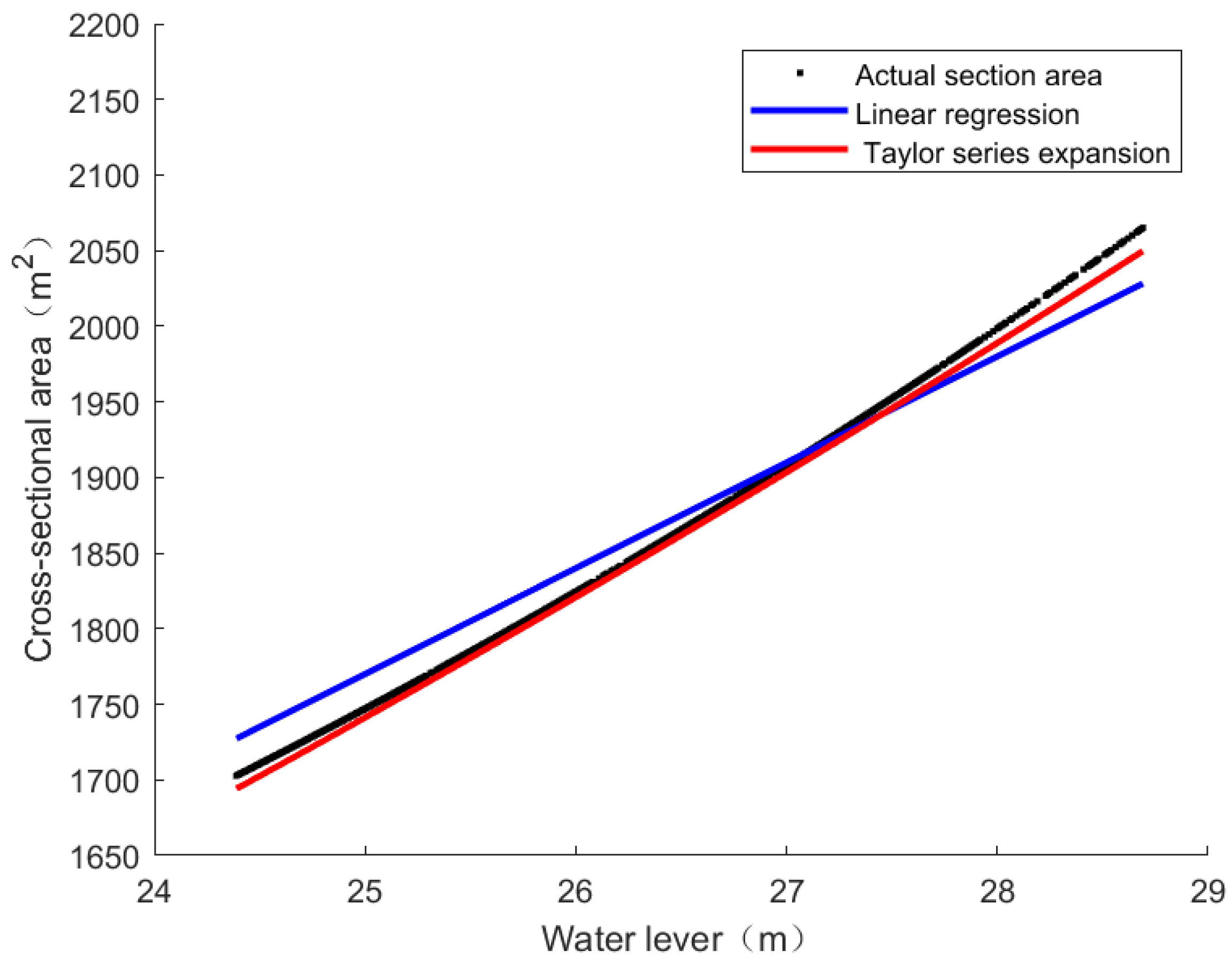
3.2. Cross-Sectional Velocity Model Fitting

To evaluate the effectiveness of the improved method, the radar data was divided into two subsets: 80% for the training set and 20% for the validation set. These subsets were randomly selected to avoid biases and ensure coverage across the entire range of water level changes. The proposed model was fitted using the least squares method by substituting river cross-sectional flow velocity and index velocity into Equations (2) and (5), respectively. Due to the impact of rainfall, the river flow rates were divided into high-water period (wet season) and low-water period (dry season) for fitting. The resulting expressions for the relationship between the average cross-sectional velocity and index velocity during the low-water period are shown in Equations (8) and (9), and those for the high-water period are shown in Equations (10) and (11).
V k 1 = 2.173 v i n d 2 h + 57.52 v i n d + 0.423
V x 1 = 0.1296 v i n d 2 3.281 v i n d + 0.7179
V k 2 = 0.598 v i n d 2 h 0.5553 v i n d + 0.6366
V x 2 = 1.58 v i n d 2 1.973 v i n d + 1.376
The comparison chart between the fitted cross-sectional flow velocity and the actual flow velocity is shown in Figure 8 and Figure 9. However, to better evaluate the model’s performance and accuracy, this paper uses the Mean Absolute Error (MAE), Root Mean Square Error (RMSE), and Nash–Sutcliffe Efficiency Coefficient (NSE) to assess the quality of the model’s predictions. For MAE and RMSE, values closer to 0 indicate better model performance. For NSE values closer to 1 signify better model performance. The relevant formula expressions are shown in Equations (12)–(14).
M A E = i = 1 n | x i y i | n
R M S E = 1 n i = 1 n ( x i y ¯ i ) 2
N S E = 1 i = 1 n ( x i y i ) 2 i = 1 n ( x i x ¯ i ) 2
In the formula: x i represents the calculated cross-sectional flow velocity, x ¯ i represents the average of the calculated cross-sectional flow velocities, y i represents the actual cross-sectional flow velocity, y ¯ i represents the average of the actual cross-sectional flow velocities, and n represents the number of samples.
Based on Table 2, it can be observed that during both the low-flow period and the high-flow period, the improved model has a smaller mean absolute error (MAE) than the pre-improvement model. For MAE, the error of the improved model has reduced by 3% compared to the pre-improvement model. Looking at the Nash–Sutcliffe model efficiency coefficient, the improved model is closer to the measured values. Hence, it can be concluded that the improved model has a better fit than the model before improvement.

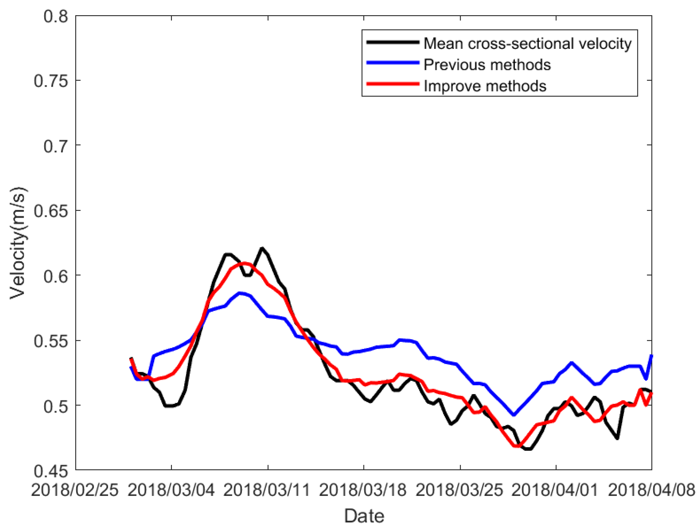
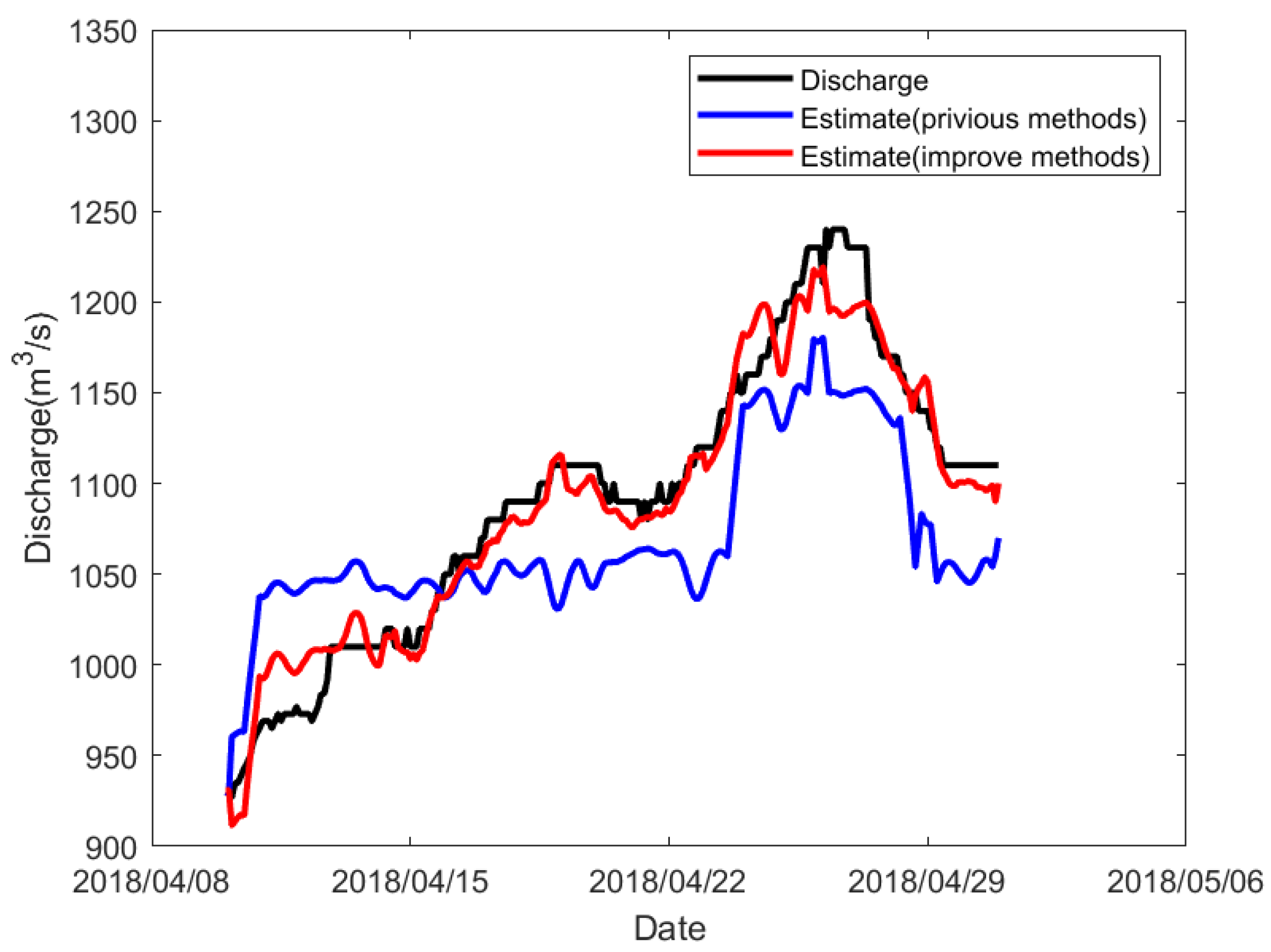
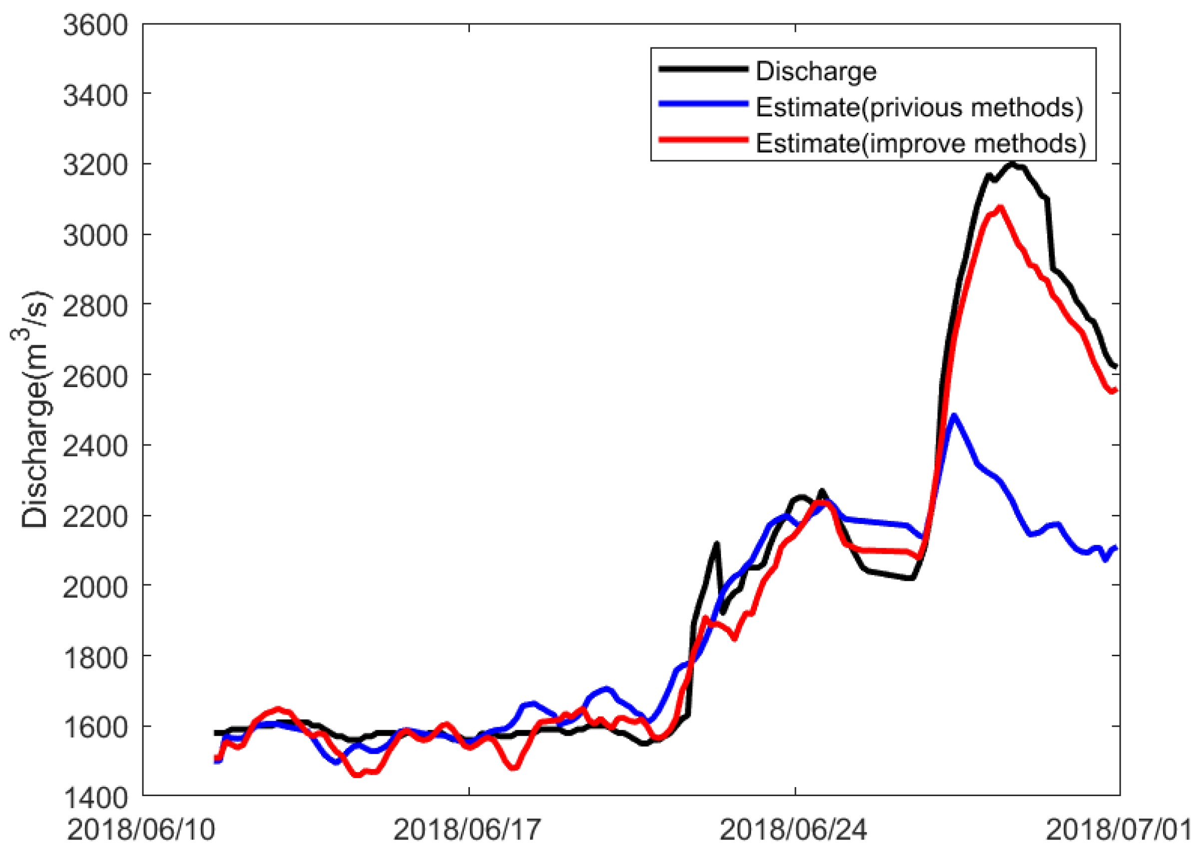
3.3. River Discharge Forecasting

For the method proposed in this article, the relationship between cross-sectional area and water level is nonlinear. The relationship graph obtained by employing Taylor series expansion for cross-sectional area and water level is shown in Figure 10.
According to the fitting model mentioned above, by substituting Equations (3) and (6) into Equation (1), the flow rate can be calculated. Evaluation metrics are assessed using the correlation coefficient, RMSE (Root Mean Square Error), and Mean Absolute Percentage Error (MAPE), as shown in Equations (15) and (16). A correlation coefficient closer to 1 indicates a better model, and smaller RMSE and MAPE indicate a better model as well. The calculated metrics are shown in Table 3.
C C = i = 1 k ( ( Q m ) i ( ( Q ¯ m ) i ) ( ( Q i ) ( Q ¯ ) i ) ( i = 1 k ( ( Q m ) i ( Q ¯ m ) i ) j = 1 k ( ( Q ) i ( Q ¯ ) i ) ) 1 2
M A P E = 100 % k i = 1 k | ( Q m ) i ( Q m ) ^ | ( Q m ) i
In the formula: Q i represents the calculated river discharge, Q m represents the river discharge provided by the hydrological station, Q ¯ i represents the average of the calculated discharge, Q ¯ m represents the average of the river discharge provided by the hydrological station, and n represents the number of samples.
To illustrate the differences between the two methods using velocity-based metrics, Figure 11 and Figure 12 show the flow measurements for approximately one month during both the low-water and high-water periods. During this period, the flow rate changes from 900 to 1250 m3 during the low-water period, and from 1400 to 3200 m3 during the high-water period. Although both methods are very close to the true values, the errors in the method after improvement are smaller than those in the method before improvement.
From Figure 11, Figure 12 and Table 3, it can be analyzed that both methods have high correlation coefficients. However, compared to the method before improvement, the method after improvement has reduced the RMSE by 25 during the low-water period and by 75 during the high-water period, and the MAPE has decreased by 2% during the low water period and by 3% during the high water period. The experimental results show that the improvements are more significant during the high-water period, possibly due to the more pronounced water level changes caused by increased rainfall. The pre-improvement method, which included water level as a factor, tends to amplify this error during the rainy season, resulting in larger errors in the calculated discharge. After the improvements, all indicators performed better than the previous method. The differences in the correlation coefficients between the two methods are not significant, but in terms of RMSE and MAPE, the improved method shows about a 2% reduction in error compared to before the improvements. Therefore, it can be concluded that the improved model provides a discharge estimation with smaller errors.

4. Discussion

Liu et al. [30] conducted a study on narrow and deep rivers in mountainous areas. They chose the average of the maximum surface flow velocity as the reference velocity. Their study also took into account the high curvature in winding river channels when selecting the reference flow velocity, and similarly, they chose the average surface flow velocity as the reference velocity. In the approximate calculation of the cross-sectional area, Liu and Yang et al. [29] used a quasi-rectangular cross-section to estimate the river’s cross-sectional area. In the estimation of the river’s cross-sectional area.
Nonetheless, the method outlined in this study also has some limitations. When using UHF radar to measure flow velocity, only the surface flow velocity of the river can be detected. Therefore, for rivers that are relatively deep or have significant undercurrents, using the surface flow velocity to estimate the cross-sectional flow velocity can result in significant errors. Secondly, UHF radar measures velocity using electromagnetic waves. Therefore, when the river flow velocity is low, the radar echoes are weak, which can lead to larger errors in the measured flow velocity. Finally, concerning the prediction of river flow, the data used in this study has a limited. This restricts the effectiveness of the predictions and prevents them from accurately reflecting long-term trends.

5. Conclusions

The focus of this experiment is to study the newly proposed method for calculating the flow of winding rivers. The conclusions derived from the comparison with the prior method are as follows:
The index-velocity for the mean velocity on the river surface is chosen and the cross-sectional velocity obtained through binary regression fitting, without incorporating water level, are closer to the actual cross-sectional flow velocity of the river. In the previous method, the water level was considered when fitting the cross-sectional velocity. During the dry season, with minimal water level changes, the impact of water level error on the cross-sectional velocity is minimal. However, during the wet season, as the river level rises, water level error can significantly impact the cross-sectional flow velocity. During the dry season, the improved method reduced the MAE from 0.0331 to 0.0094, the RMSE from 0.251 to 0.0124, and increased the NSE from 0.5902 to 0.9228 compared to the previous method. During the wet season, the improved method reduced the MAE from 0.0546 to 0.0355, the RMSE from 0.0762 to 0.0359, and increased the NSE from 0.8578 to 0.9555 compared to the previous method.
This indicates that the improved method is more effective in predicting the cross-sectional velocity in curved river channels. After obtaining the river cross-sectional flow velocity, we propose using a Taylor series expansion to fit the nonlinear relationship between cross-sectional area and water level. Compared to the previous method, the improved approach increased the CC from 0.8280 to 0.9523, reduced the RMSE from 48.1057 to 23.0383, and decreased the MAPE from 0.0473 to 0.0232 during the dry season. During the wet season, the CC increased from 0.9333 to 0.9908, the RMSE decreased from 140.62 to 65.4929, and the MAPE dropped from 0.0729 to 0.0391. This suggests that utilizing a Taylor series expansion for nonlinear calculations can more effectively minimize the errors associated with linear approximation fitting.
The study’s findings enhance river flow calculations with non-contact measurement techniques and extend the use of ultra-high frequency surface wave radar in analyzing curved river channels.

Author Contributions

K.L. proposed the methodology, conducted the experiment, prepared figures, and wrote the manuscript. Z.L. reviewed the manuscript. All authors have read and agreed to the published version of the manuscript.

Funding

This work was supported in part by National Natural Science Foundation of China (NSFC) (NO. 62361006), in part by Guangxi Natural Science Foundation under grant 2020GXNSFBA297119.

Data Availability Statement

Due to privacy concerns, the data from this study are not publicly available. The sensitivity of the data and the need to protect privacy prevent us from sharing the data. If you have any questions or require further information, please contact the corresponding author of this paper.

Conflicts of Interest

The authors declare no conflicts of interest.

References

  1. Aguilera, R.; Melack, J.M. Relationships among nutrient and sediment fluxes, hydrological variability, fire, and land cover in coastal California catchments. J. Geophys. Res. Biogeosci. 2018, 123, 2568–2589. [Google Scholar] [CrossRef]
  2. Allen, G.H.; Pavelsky, T.M. Global extent of rivers and streams. Science 2018, 361, 585–588. [Google Scholar] [CrossRef]
  3. Haddel, I.; Clark, D.B.; Franssen, W.; Ludwig, F.; Voß, F.; Arnell, N.W.; Bertr, N.; Best, M.; Folwell, S.; Gerten, D.; et al. Multimodel estimate of the global terrestrial water balance: Setup and first results. J. Hydrometeorol. 2011, 12, 869–884. [Google Scholar] [CrossRef]
  4. Vyas, J.K.; Perumal, M.; Moramarco, T. Non-contact discharge estimation at a river site by using only the maximum surface flow velocity. J. Hydrol. 2024, 638, 131505. [Google Scholar] [CrossRef]
  5. Fulford, J.M.; Thibodeaux, K.G.; Kaehrle, W.R. Comparison of current meters used for stream gaging. In Proceedings of the Symposium on Fundamentals and Advancements in Hydraulic Measurements and Experimentation, Buffalo, NY, USA, 1–5 August 1994; pp. 376–385. [Google Scholar]
  6. Vermeulen, B.; Sassi, M.G.; Hoitink, A.J.F. Improved flow velocity estimates from moving-boat ADCP measurements. Water Resour. Res. 2014, 50, 4186–4196. [Google Scholar] [CrossRef]
  7. Lin, H.; Cheng, X.; Liu, J.; Shi, Q.; Li, T.; Zheng, L.; Hou, X.; Du, J. Estimating river discharge across scales with a novel regional gauging method driven by Sentinel satellite data. Remote Sens. Environ. 2024, 311, 114266. [Google Scholar] [CrossRef]
  8. Xu, J.; Wang, L.; Yao, T.; Chen, D.; Wang, G.; Jing, Z.; Zhang, F.; Wang, Y.; Li, X.; Zhang, Y.; et al. Totaling river discharge of the third pole from satellite imagery. Remote Sens. Environ. 2024, 308, 114181. [Google Scholar] [CrossRef]
  9. Sichangi, A.W.; Wang, L.; Yang, K.; Chen, D.; Wang, Z.; Li, X.; Zhou, J.; Liu, W.; Kuria, D. Estimating continental river basin discharges using multiple remote sensing data sets. Remote Sens. Environ. 2016, 179, 36–53. [Google Scholar] [CrossRef]
  10. Keulegan, G.H. Laws of Turbulent Flow in Open Channels. J. Res. Natl. Bur. Stand. 1938, 21, 707–741. [Google Scholar] [CrossRef]
  11. Cheng, N.S. Power-Law Index for Velocity Profiles in Open Channel Flows. Adv. Water Resour. 2007, 30, 1775–1784. [Google Scholar] [CrossRef]
  12. Bonakdari, H.; Larrarte, F.; Lassabatere, L.; Joannis, C. Turbulent Velocity Profile in Fully-Developed Open Channel Flows. Environ. Fluid Mech. 2008, 8, 1–17. [Google Scholar] [CrossRef]
  13. Coles, D. The Law of the Wake in the Turbulent Boundary Layer. J. Fluid Mech. 1956, 1, 191–226. [Google Scholar] [CrossRef]
  14. Wang, S.; Wen, B.; Wang, C.; Zhou, Y. UHF Surface Dynamics Parameters Radar Design and Experiment. IEEE Microw. Wirel. Compon. Lett. 2014, 24, 65–67. [Google Scholar] [CrossRef]
  15. Zhang, Y.; Zhou, Y. Automatic Flow Detection System for Rectangular Channels Based on the Five-Point Method. Chin. Rural Water Hydropower 2014, 5, 115–117. [Google Scholar]
  16. Sarma, K.V.N.; Lakshminarayana, P.; Rao, N.S.L. Velocity Distribution in Smooth Rectangular Open Channels. J. Hydraul. Eng. 1983, 109, 270–289. [Google Scholar] [CrossRef]
  17. Levesque, V.A.; Oberg, K.A. Computing Discharge Using the Index Velocity Method; US Department of the Interior, US Geological Survey: Reston, VA, USA, 2012.
  18. Teague, C.C.; Barrick, D.E.; Lilleboe, P.M.; Cheng, R.T.; Ruhl, C.A. UHF RiverSonde observations of water surface velocity at Threemile Slough, California. In Proceedings of the IEEE International Geoscience and Remote Sensing Symposium, Seoul, Republic of Korea, 29 July 2005; Volume 50, pp. 4186–4196. [Google Scholar]
  19. Fulton, J.W.; Mason, C.A.; Eggleston, J.R.; Nicotra, M.J.; Chiu, C.L.; Henneberg, M.F.; Best, H.R.; Cederberg, J.R.; Holnbeck, S.R.; Lotspeich, R.R.; et al. Near-field remote sensing of surface velocity and river discharge using radars and the probability concept at 10 US geological survey streamgages. Remote Sens. 2022, 12, 1296. [Google Scholar] [CrossRef]
  20. Alimenti, F.; Bonafoni, S.; Gallo, E.; Palazzi, V.; Gatti, R.V.; Mezzanotte, P.; Roselli, L.; Zito, D.; Barbetta, S.; Corradini, C.; et al. Noncontact Measurement of River Surface Velocity and Discharge Estimation With a Low-Cost Doppler Radar Sensor. IEEE Trans. Geosci. Remote Sens. 2022, 58, 5195–5207. [Google Scholar] [CrossRef]
  21. Qiu, J.; Long, K.; Du, Y.; Xie, H.; Wei, Z.; Shangguan, W.; Dai, Y. A hybrid deep learning algorithm and its application to streamflow prediction. J. Hydrol. 2021, 601, 126636. [Google Scholar]
  22. Alizadeh, F.; Gharamaleki, A.F.; Jalilzadeh, R. A two-stage multiple-point conceptual model to predict river stage-discharge process using machine learning approaches. J. Water Clim. Chang. 2021, 12, 278–295. [Google Scholar] [CrossRef]
  23. Difi, S.; Elmeddahi, Y.; Hebal, A.; Singh, V.P.; Heddam, S.; Kim, S.; Kisi, O. Monthly streamflow prediction using hybrid extreme learning machine optimized by bat algorithm: A case study of Cheliff watershed, Algeria. Hydrol. Sci. J. 2022, 68, 189–208. [Google Scholar] [CrossRef]
  24. Shabbir, M.; Chand, S.; Iqbal, F. A novel hybrid method for river discharge prediction. Water Resour. Manag. 2022, 36, 253–272. [Google Scholar] [CrossRef]
  25. Mutschler, M.A.; Scharf, P.A.; Rippl, P.; Gessler, T.; Walter, T.; Waldschmidt, C. River Surface Analysis and Characterization Using FMCW Radar. IEEE J. Sel. Top. Appl. Earth Obs. Remote Sens. 2022, 15, 2493–2502. [Google Scholar] [CrossRef]
  26. Le Coz, J.; Camenen, B.; Peyrard, X.; Dramais, G. Uncertainty in open-channel discharges measured with the velocity–area method. Flow Meas. Instrum. 2012, 26, 18–29. [Google Scholar] [CrossRef]
  27. Ruhl, C.A.; Simpson, M.R. Computation of Discharge Using the Index-Velocity Method in Tidally Affected Areas; US Department of the Interior, US Geological Survey: Denver, CO, USA, 2005.
  28. Morse, B.; Hamai, K.; Choquette, Y. River discharge measurement using the velocity index method. In Proceedings of the 13th CRIPE Workshop on the Hydraulics of Ice Covered Rivers, Hanover, NH, USA, 15–16 June 2005. [Google Scholar]
  29. Yang, Y.; Wen, B.; Wang, C.; Hou, Y. Real-Time and Automatic River Discharge Measurement With UHF Radar. IEEE Geosci. Remote Sens. Lett. 2022, 17, 1851–1855. [Google Scholar] [CrossRef]
  30. Liu, C.; Wen, B.; Duan, Z.; Tian, Y. Measurement of Mountain River Discharge Based on UHF Radar. IEEE Geosci. Remote Sens. Lett. 2023, 20, 1–5. [Google Scholar] [CrossRef]
  31. Ma, M.; Li, G.; Ning, J. Large-Eddy Simulation of Hydrodynamic Structure in a Strongly Curved Bank. Appl. Sci. 2022, 12, 11883. [Google Scholar] [CrossRef]
  32. Sy, E. River Water Surface Velocity Measurement Using Large-Scale Particle Image Velocimetry. 2024. Available online: https://mspace.lib.umanitoba.ca/items/3aea13aa-8be1-487f-bf28-e9c67f457b69 (accessed on 21 July 2024).
  33. Zhang, E.; Li, L.; Huang, W.; Jia, Y.; Zhang, M.; Kang, F.; Da, H. Measuring Velocity and Discharge of High Turbidity Rivers Using an Improved Near-Field Remote-Sensing Measurement System. Water 2024, 16, 135. [Google Scholar] [CrossRef]
Figure 1. Ideal river cross-sectional area.
Water 16 02361 g001
Figure 2. Curved river channel cross-sectional area.
Water 16 02361 g002
Figure 3. Deployment of ultra-high frequency radar schematic.
Water 16 02361 g003
Figure 4. Cross-section of the channel.
Water 16 02361 g004
Figure 5. Study area of the river.
Water 16 02361 g005
Figure 6. Water level and cross-sectional area provided by the Xiantao Hydrologic Station.
Water 16 02361 g006
Figure 7. Cross-sectional area and discharge provided by the Xiantao Hydrologic Station.
Water 16 02361 g007
Figure 8. Comparison between the estimated cross-sectional river velocity and the velocity provided by the Hubei Xiantao Hydrologic Station during the dry season.
Water 16 02361 g008
Figure 9. Comparison between the estimated cross-sectional river velocity and the velocity provided by the Hubei Xiantao Hydrologic Station during the wet season.
Water 16 02361 g009
Figure 10. Taylor expansion approximation results for the S-h relationship.
Water 16 02361 g010
Figure 11. Comparison between the estimated discharge and the discharge provided by the Hubei Xiantao Hydrologic Station during the dry season.
Water 16 02361 g011
Figure 12. Comparison between the estimated discharge and the discharge provided by the Hubei Xiantao Hydrologic Station during the wet season.
Water 16 02361 g012
Table 1. OSMAR-SU waveform parameters of ultra high frequency radar.
Operating FrequencyValue
Operating frequency f (MHz)340
Sweep bandwidth B (MHz)15
Sweep width  T s (ms)41
Sweep period T (ms)40
Maximum detection range  R m a x (m)500
Range resolution  Δ R (m)10
Maximum detection speed  v m a x (m/s)5.489
Speed resolution  Δ v (m/s)0.0214
Table 2. Performance evaluation of velocities calculated by different models.
TimeDry SeasonWet Season
MethodPreviousImprovePreviousImprove
MAE0.03310.00940.05460.0355
RMSE0.02510.01240.07620.0359
NSE0.59020.92280.85780.9555
Table 3. Statistical results of radar discharge measurement.
TimeDry SeasonWet Season
MethodPreviousImprovePreviousImprove
CC0.82800.95230.93330.9908
RMSE48.105723.0383140.6265.4929
MAPE0.04730.02320.07290.0391
Disclaimer/Publisher’s Note: The statements, opinions and data contained in all publications are solely those of the individual author(s) and contributor(s) and not of MDPI and/or the editor(s). MDPI and/or the editor(s) disclaim responsibility for any injury to people or property resulting from any ideas, methods, instructions or products referred to in the content.

