Abstract
Climate change and anthropogenic impacts drastically affect the biogeochemical regime of the Black Sea, which contains the largest volume of sulphidic water in the world. The Sea’s oxygen inventory depends on vertical mixing that transports dissolved oxygen (DO) from the upper euphotic layer to deeper layers and on dissolved oxygen consumption for the oxidation of organic matter (OM) and reduced species of S, Fe, and Mn. Here we use a vertical one-dimensional transport model, 2DBP, forced by Copernicus data, that was coupled with the FABM-family N-P-Si-C-O-S-Mn-Fe Bottom RedOx Model BROM. The research objective of this study was to analyze the oxygen budget in the upper 350 m of the Sea and demonstrate the role of the parameterization of the acceleration of the sinking of particles covered by precipitated Mn(IV). The analysis of the oxygen budget revealed distinct patterns in oxygen consumption within different depths. In the oxic zone, the primary sink for DO is the mineralization of organic matter, whereas in the suboxic zone, dissolved Mn(II) oxidation becomes the predominant sink. The produced Mn(IV) sinks down and reacts with hydrogen sulphide several meters below, making possible the existence of the suboxic layer without detectable concentrations of DO and H2S.
1. Introduction
The Black Sea is an inland sea that is permanently stratified by the large river runoffs at the surface and saline Mediterranean water influx, with the bottom current in the Bosphorus Strait. The existence of a permanent halocline limits the influence of the river discharges and atmospheric forcing to the upper 100–150 m of the water column, resulting in pronounced seasonal variations [1], while the deeper water contains the largest volume of sulphidic water in the world. Therefore, the sea’s surface waters and the deep waters are decoupled, and the residence time increases from a few years for the layer of the main halocline [2,3] to several hundred years for the deepest layer [4]. This feature of the vertical structure distinguishes the Black Sea from other marine environments.
Annual renewal of the surface waters extends only to depths of 60–80 m, coinciding with the cold intermediate layer (CIL) ( = 14.50 kg/m). Below this depth, turbulent diffusion governs vertical fluxes, limiting the oxygen supply and causing rapid depletion due to the oxidation of organic matter (OM) and reactions with reduced species of nitrogen, manganese, iron, and sulphur sourced from deeper layers. Hydrogen sulphide begins to appear around 50 m below the CIL (∼110 to 130 m), marking the onset of euxinic conditions [5].
A defining feature of the Black Sea is the formation of a transitional redox layer, or pelagic redoxcline, where the redox potential decreases with the depth (and density), marking the transition from oxic to anoxic conditions and facilitating complex interactions among oxidized and reduced chemical species [6,7]. This layer plays a key role in the biogeochemical cycling of oxygen and other elements, influencing nutrient dynamics and ecosystem processes throughout the water column. The processes in the redox zone occur in a predictable sequence depending on changes in redox potential [6,7]. Organic matter, the main reducing agent in the redox zone, is transported from the euphotic zone as a new production and is also generated by chemosynthesis within the redox zone.
One of the most interesting properties of the Black Sea redox zone is the suboxic layer, first described by the 1988 RV Knorr Expedition [8]. This zone is characterized by low oxygen concentrations (<10 M) and minimal hydrogen sulphide levels (<0.3 M), serving as a boundary between the oxic and sulphidic layers. The formation of this layer is attributed to the interactions between manganese compounds, oxygen, and hydrogen sulphide [9,10].
A characteristic feature of the Black Sea, excluding the Bosporus Strait area, is that chemical and biological processes in the redox zone occur within narrow density layers (2–5 m), a correspondence known as chemotrophy [6,7,11,12,13,14,15,16,17]. This correspondence between chemical profiles and water density facilitates the application of one-dimensional conceptual and numerical models to understand the biogeochemical dynamics.
The biogeochemical regime of the Black Sea is increasingly affected by the complex interactions of climate change and anthropogenic impacts. Changes in temperature, wind patterns, stratification, storm activity, the hydrological cycle, and intensified eutrophication from anthropogenic nutrient supply pose significant challenges to ecosystem resilience [18,19,20,21]. Furthermore, the oxygen budget is highly sensitive to these changes, highlighting the importance of understanding the effect of different processes on the oxygen budget and dynamics.
Over the past few decades, different mathematical models have been developed to study the biogeochemical and ecosystem dynamics of the Black Sea. These models vary in their degree of complexity, from one-dimensional Fasham-like models of the oxic layer to three-dimensional models [1,5,22,23,24,25,26,27,28,29,30]. These models have been able to reproduce fundamental features of the water column and the pelagic redox interface [9] and have contributed to understanding the impacts of climate change and anthropogenic pressures on the oxygen inventory, including the shallowing of the oxygen penetration depth [24].
In this study, our objective is to model the biogeochemical structure of the upper 350 m of the Black Sea, with a specific focus on the redox layer, and to analyze the effect of different processes on the oxygen budget. Additionally, we aim to investigate the impact of particulate manganese precipitation on the vertical distribution of biogeochemical species. For this purpose, we conduct numerical simulations using the benthic–pelagic biogeochemical model BROM, selected for its capability to accurately replicate the processes at the redox interfaces. This model is based on previous work on modeling the Black Sea’s biogeochemistry [22,23,31,32], with a new hydrodynamical approach based on an up-to-date Copernicus Black Sea Physical Reanalysis (version E3R1) [33].
2. Methods
2.1. Model Description
We coupled the biogeochemical model BROM with the two-dimensional benthic–pelagic transport model 2DBP, resulting in the integrated model 2DBP–BROM. This model operates within the modular Framework for Aquatic Biogeochemical Models (FABM) [34], which facilitates the use of different models as reusable components, including the transport 2DBP module and the BROM ecological and biogeochemical modules.
2.2. Transport Model
The two-dimensional benthic–pelagic model (2DBP) simulates the vertical and horizontal transport of particulate and dissolved matter in the water column and upper sediments at small horizontal scales [22]. In this study, we employ only a one-dimensional approach, dividing the water column grid into layers of variable depth (1 to 100 m), with an increasing resolution in the pelagic redoxcline (Figure 1). Vertical transport results from two mechanisms: vertical diffusivity and particulate matter sinking. Vertical diffusivity is estimated from temperature and salinity data using the Gargett formula (Equation (1)) [35].
where N is the buoyancy frequency, g is the acceleration of gravity, is the mean density, and and q are empirical coefficients. This approach was successfully used for studying the vertical physical [36] and biogeochemical structure [9] of the Black Sea.
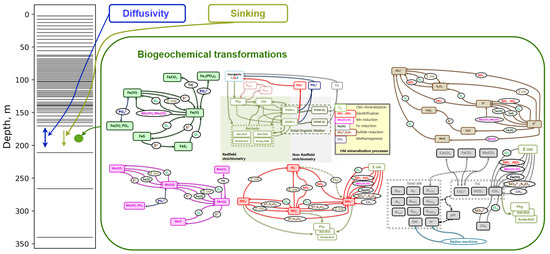
Figure 1.
Model setup scheme. On the left-hand side, the calculation grid is presented. In each grid cell, sinking, diffusivity and biogeochemistry processes are parmeterized following Equation (2). One can find a detailed description of biogeochemical transformations in model BROM in [22].
An overall equation of the model is
where is the concentration of the i-th model state variable, is the sinking rate, is the vertical turbulence coefficient, and is the biogeochemical “sources-minus-sinks” term.
2.3. Biogeochemical Model
The benthic–pelagic biogeochemical model BROM integrates a relatively simple pelagic ecosystem model with a comprehensive biogeochemical model that simulates the water column, benthic boundary layer, and sediments, with a particular emphasis on oxygen dynamics and redox conditions. BROM accounts for the coupled cycling of multiple chemical species, including nitrogen (N), phosphorus (P), silica (Si), carbon (C), oxygen (O), sulphur (S), manganese (Mn), and iron (Fe). The model quantifies organic matter (OM) using nitrogen as the currency while adhering to the Redfield ratios that govern the stoichiometric relationships between the major nutrients (Figure 1). The model BROM incorporates parameterizations for organic matter (OM) dynamics, including production processes such as photosynthesis and chemosynthesis, as well as decay pathways like oxic mineralization, denitrification, manganese reduction, iron reduction, sulphate reduction, and methanogenesis. To capture the changing redox conditions in detail, BROM simulates the mineralization of OM using multiple electron acceptors, and dissolved oxygen is consumed during both the mineralization of OM and the oxidation of various reduced compounds. Within the model, OM is represented as dissolved labile OM, dissolved semi-labile OM, particulate labile OM, and particulate semi-labile OM, providing a comprehensive characterization of the organic matter pool. Adopting a similar approach to the ERSEM model, the decay of labile organic matter forms in BROM leads to the release of phosphate and ammonium, as well as the transformation of labile forms into semi-labile forms. During the decay process of organic matter (OM), electron acceptors are consumed and carbon dioxide is released. This feature enables the model to account for deviations from the Redfield stoichiometry during OM mineralization. The inhibition of biogeochemical processes is parameterized using a set of redox-dependent switches, which are modulated by the redox potential. Furthermore, BROM incorporates a module that describes carbonate equilibria, allowing the model to investigate acidification processes and the impacts of changing pH and saturation states on the biogeochemistry of water and sediments. A detailed description of BROM is given in [22]. The list of the model state variables is given in Table A1.
A common feature of the redox interface is the presence of a Mn(IV) maximum [37]. Typically, Mn(IV) particles are formed in the oxic zone through the oxidation of dissolved Mn(II). These particles then sink down to the sulphidic layer, where they are reduced back to Mn(II). Due to its high density, which is about 7 times higher than that of organic matter, Mn(IV) accelerates the sinking of other particles present in the redoxcline [38]. This mechanism is important for understanding the absence of both oxygen and hydrogen sulphide in the suboxic layer.
To model the accelerated sinking of particles, we implement the following equation:
where — the total vertical velocity, — the intrinsic vertical velocity of the suspended matter type, — the intrinsic vertical velocity of the Mn(IV), – Mn(IV) oxide concentration, and = 0.1 M (empirical coefficient). Particulate matter types: S, MnS, MnCO, Fe(III), FeS, FeCO, Fe(PO) CaCO, POM, and plankton species. The presented equation is just an addition of the intrinsic vertical velocity of the suspended matter type and an additional velocity term. The last is a Monod term that depends on the Mn(IV) concentration. A similar approach is used in [9] and based on field observations [37]. We deliberately ignore Fe particulated species due to their small contribution to the redox exchange [37].
2.4. Model Setup
The 2DBP–BROM model was configured for a location in the Black Sea, focusing on the upper 350 m of the water column, comprising the surface oxygenated layer, pelagic redoxcline, and sulphidic bottom environment. The model was driven by sea temperature and salinity data obtained from the Copernicus Black Sea Physical Reanalysis (version E3R1) [33] for 2003 for a point with the coordinates 42.0° N 30.5° E. A simulation was initialized with vertically homogeneous conditions and run until a quasi-stationary solution was reached after 50 model years. The model results were validated by comparing them with in-situ measurements from the 2003 RV “Knorr” field expedition [39].
3. Results and Discussion
3.1. Comparison with the Observations Data
The modeled vertical distributions of dissolved oxygen, hydrogen sulphide, and dissolved Mn(II) were compared with measurements from the Western Black Sea Gyre in March 2003 [39]. The modeled dissolved oxygen shows a comparable profile to the observations, decreasing from approximately 300–350 M at the surface to complete depletion at the 15.7 kg/m isopycnic level. Mn(II) first appears at the density level of 15.9 kg/m, reaching 6 M at = 16.1 kg/m in the model, compared with 5–8 M at = 16.5 kg/m in the observations, indicating the shallower position of the Mn(II) maximum in the model. Hydrogen sulphide initially appears at a density level of 16.1 kg/m and increases with depth, exhibiting similar behavior in both the model and observations. These results demonstrate the capability of the model to reproduce the vertical distribution of these variables during winter (Figure 2).
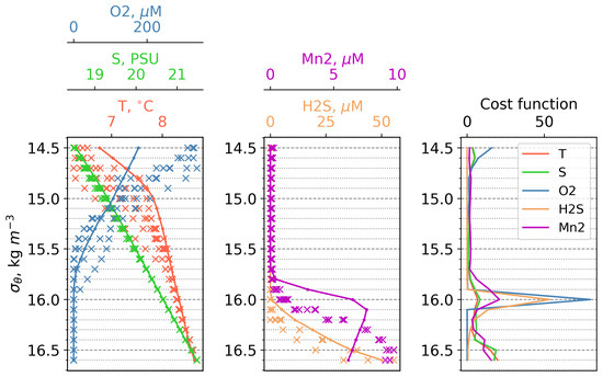
Figure 2.
Left and center plots: First vertical distributions of temperature, salinity, dissolved oxygen, bivalent manganese, and hydrogen sulphide in density coordinates. Lines refers to model data, “x” to observations of the expedition on the RV “Knorr” in March 2003. All data interpolated on the same density levels. Right plot: Vertical distributions of cost function for salinity, dissolved oxygen, bivalent manganese, and hydrogen sulphide in density coordinates.
We validated our results using the cost function (Equation (4)) method employed in the work [40].
where is the model mean, is the averaged observation data, and is the standard deviation of the observation data. This method is convenient for assessing the closeness of the obtained model solution to the observation data in the absence of a large amount of the latter. In fact, it checks whether the difference between the model solution and the selected validation data falls outside the standard deviation of the latter. The following scale is recommended for this method: a from 0 to 1—good; from 1 to 2—reasonable; 2 and above—poor [40].
Before averaging, we interpolated the model data and observation data onto density levels, then averaged the model data for March and the observation data for the available stations. The vertical distributions of the resulting cost functions (C) are shown in (Figure 2). The horizons that contribute the most weight to the cost function can be seen in Figure 2.
First of all, it must be noted that the hydrophysical forcing data from Copernicus used in the model correspond to a typical year, while during the observations in 2003, it was a very cold year that included the renovation of the Black Sea CIL [39]. That is why, in 1 t 14.5, there is a strong discrepancy in the DO, which is most likely caused by the increased temperature of the model input data compared with the Knorr cruise data (Figure 2). The next critical section is density level 16.0. This huge maximum is explained by a combination of unpleasant features: (1) the input series T and S—this leads to a slight shift in the position of the oxycline, which, under the conditions of a strong gradient of the characteristic, is expressed in an increased deviation from the observation data; and (2) the extremely low standard deviations for chemical compounds in the observation data, which leads to division by a small number and huge values of C. All large values of C below the 16.0 horizon are explained by the same reason, but simply on a smaller scale than at the 16.0 horizon. We suppose that the main reason for the difference between the onset depths of Mn2 and H2S in the model and in the observations is connected with the forcing of our 1D model with the hydrophysics produced by a model (Copernicus reanalysis that has deviations from the observations). Nevertheless, as it was discussed above, our results correctly reflect the main features of the vertical distributions of the biogeochemical parameters.
The vertical distribution of all model state variables during summer is shown in Figure 3. The cold intermediate layer spans depths between 10 and 50 m, while the oxygenated layer extends from the surface to 90 m, with the oxycline being observed between 40 and 80 m below the cold intermediate layer. NO increases from 1 M in the surface layer to a maximum of 4 M at an 80 m depth. NO is only detected between an 80 and 90 m depth, while NH, in the absence of oxygen, begins to increase, reaching 50 M at a 270 m depth. Modeled concentrations of PON and DON (0.4 M and 10 M, respectively) generally correspond to those observed in the Black Sea [17,41].
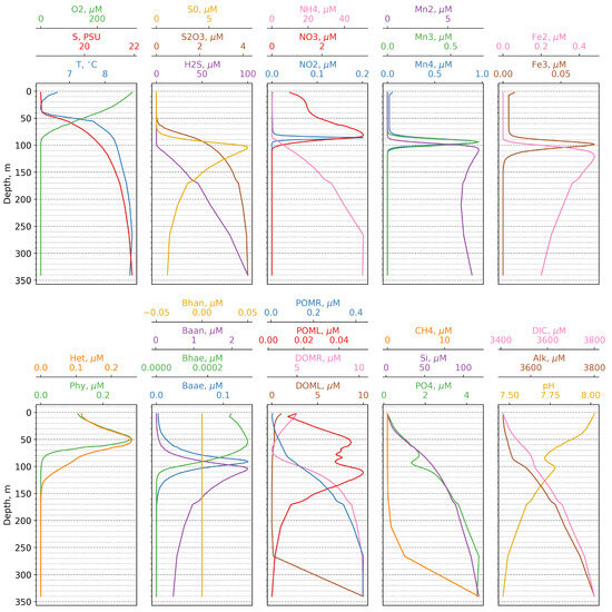
Figure 3.
Calculated vertical distributions of the model state variables versus depth.
In the model, the suboxic zone, where hydrogen sulphide and oxygen are absent, can be found between a 90 and 105 m depth. S first appears at around 70 m, peaks at 105 m with a value of 10 M, and then decreases to 2 M at 300 m, which is within the range of values observed in the Black Sea [42]. Thiosulphate, an intermediate product of sulphate reduction and sulphide oxidation, appears at 60 m in the oxic zone and increases to 6 M at 300 m.
Mn(II) first appears at 90 m and, after peaking at about 110 m, maintains relatively constant concentrations throughout the sulphidic layer (Figure 3). Mn(III) and Mn(IV) exhibit similar distributions, being observed exclusively above the sulphidic layer at depths between 80 and 110 m. The simulated values for the manganese compounds fall within the ranges reported in the literature [9,43,44,45]. The vertical distributions of Fe species follow a similar pattern to that of manganese compounds. Maximum concentrations of Fe(III) (0.07 M) correspond to those reported by observations [43]. However, the depths at which both manganese and iron compounds first appear are slightly deeper than those reported in observations [13,43].
The model successfully reproduces the phosphate dipole, with phosphate showing a minimum value at around 100 m and a maximum at 250 m. Additionally, the model predicts a steep increase in phosphate concentrations at the onset of the sulphidic layer, which is consistent with observations.
Regarding functional ecological groups, the biomass of phytoplankton and zooplankton varies seasonally between 50 and 250 mg/m, while the biomass of different bacterial groups ranges from 5 to 10 mg/m. Overall, these results are in agreement with field measurements [46].
Overall, the model successfully reproduces the fundamental characteristics of the vertical structure of the pelagic redoxcline as reported in the literature [5]. Specifically, it captures (i) the correspondence between the depths of the nitrate maximum and the oxycline, (ii) the simultaneous appearance of Mn(II) and NH4+ at the same depth, and (iii) the rapid increase in phosphate below the onset of the sulphidic layer. Additionally, the model accurately simulates the sequence of electron acceptor consumption (O-NO-Mn(IV)-Fe(III)) and the appearance of electron donors (Mn(II)-NH-Fe(II)-H2S), corresponding to the theoretical “electron tower” sequence [47]. Furthermore, modeled maxima for Mn(IV), Fe(III), and anaerobic autotrophic bacteria coincide with the depth of the turbidity layer, as observed in previous studies [6,8,15,16] (Figure 4).
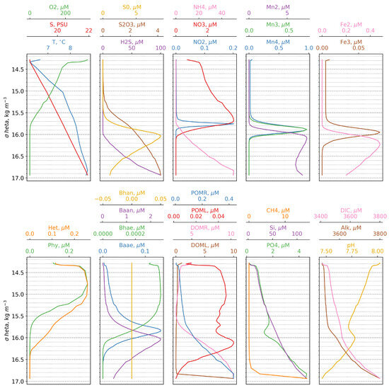
Figure 4.
Calculated vertical distributions of the model state variables versus density.
3.2. Seasonal Variability
Figure 5 illustrates the seasonal variability of key state variables. Between April and May, oxygen penetrates to a depth of up to 80 m as water oxygenation increases due to colder temperatures and the recent phytoplankton bloom that raises oxygen levels above the pycnocline. The oxygenated layer contracts to the upper 50 m by the end of summer due to the increased respiration associated with organic matter remineralization. Changes in pH within the oxic zone correlate with fluctuations in oxygen levels, as the production and consumption of organic matter affect both oxygen and CO levels, thereby influencing pH. In the suboxic zone, however, pH variations are disconnected from changes in oxygen and instead reflect changes in proton concentrations resulting from successive redox reactions [22]. The upper boundary of the sulphidic zone generally follows the trend of the oxygen layer with a delay of 1–2 months.
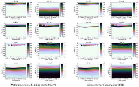
Figure 5.
Calculated seasonal variability of O2, H2S, Mn(IV), NO3, Phy, pH, S0, and, PO with accelerated sinking due to presence of Mn(IV) (right column) and without accelerated sinking due to presence of Mn(IV) (left column).
The effect of modeling the accelerated sinking of particles associated with the settling of particulate Mn(IV) is shown in Figure 5 and Figure 6. Incorporating this feature results in a narrower distribution and decreased concentration of Mn(V). The phosphate dipole is also more pronounced (Figure 5). Additionally, the redox layer decreases its depth by 0.2 density units, leading to changes in the penetration depth of oxygen that closely align with observations. Therefore, modeling the effect of accelerated sinking associated with the settling of particulate Mn(IV) improves the modeled distribution of key biogeochemical variables in the suboxic zone.

Figure 6.
Difference between experiment and base calculations in O2, H2S, Mn(IV), and NO3 seasonal variability, where experiment includes accelerated sinking velocity and base does not.
3.3. Oxygen Consumption
We investigated the effect of different processes on the oxygen budget. Figure 7 illustrates the vertical distribution of the rate of oxygen consumption associated with each process. While oxygen production through photosynthesis is observed in the upper layers (15.5 kg/m), consumption processes peak in deeper regions around 15.8 kg/m. Organic matter mineralization was identified as the primary consumer of dissolved oxygen, accounting for approximately 50.2% of the total oxygen consumption (see Figure 8). Both stages of nitrification consume around 20.5% of the available oxygen at the bottom of the oxic zone, followed by manganese oxidation, which consumes 12.8% (Figure 7 and Figure 8).

Figure 7.
Oxygen production/consumption profile in the water column from 0 to 100 m. Positive values correspond to oxygen consumption and negative ones to oxygen production.
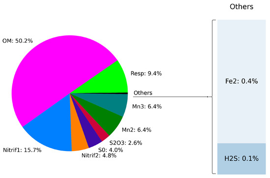
Figure 8.
Oxygen production/consumption budget in the water column from 0 to 100 m.
In the suboxic layer, where O concentrations are below 30 M above the sulphidic layer, photosynthesis is absent and respiration becomes negligible (see Figure 9 and Figure 10). In this zone, less oxygen is consumed for organic matter mineralization (approximately 25.9%), while consumption for the oxidation of reduced species and nitrification increases. A significant proportion of oxygen (43.5%) is utilized for the oxidation of both Mn(II) and Mn(III), contrasting with 12.8% in the oxic layer. Both stages of nitrification exhibit oxygen consumption levels similar to those observed in the oxic layer (21.7%), while the oxidation of iron becomes negligible (Figure 9 and Figure 10).

Figure 9.
Oxygen consumption profile in the water column in suboxic layer (O < 30 M). Positive values correspond to oxygen consumption and negative ones to oxygen production.

Figure 10.
Oxygen consumption budget in the water column in suboxic layer (O < 30 M).
The estimates of the seasonal dynamics of the biogeochemical components of the Black Sea and dissolved oxygen consumption obtained in this work demonstrate the adequacy of the biogeochemical model and the introduced parameterization, as they align with previous studies on this topic [9,48] and are available for rational interpretation. However, a comprehensive analysis of the oxygen balance in the Black Sea requires more realistic hydrophysical conditions due to the strong dependence of oxygen on wind speed, temperature distribution, and density, as mentioned in the introduction and evidenced by the model validation results based on field data.
It is also essential to consider the field hydrochemical data themselves. The most challenging aspect of verifying the model in the redox layer is finding accurate oxygen data. The difficulty in obtaining such data arises from (1) the redox layer being relatively thin compared with the depth of the sea, complicating sampling, and (2) the fact that the Winkler method for measuring dissolved oxygen concentration is still predominantly used for most measurements in the Black Sea, which does not allow for the use of data series to study the redox layer due to the high detection limit of the method. This lack of quality observational data may represent the greatest uncertainty in studying the redox layer, allowing for broad interpretations of the results from various experiments, including those involving mathematical modeling.
4. Conclusions
The results described above demonstrate the capability of the BROM model to reproduce the vertical distribution and dynamics of key biogeochemical tracers in the Black Sea. This allowed for the quantification of the effect of different processes in the oxygen budget.
The application of this model in this study provides a mechanistic understanding of the existence of the suboxic zone and the lack of direct contact between the oxic and hydrogen sulphide layers. In the suboxic zone, dissolved oxygen is primarily consumed in the oxidation of the intermediate compounds Mn(II) and Mn(III), resulting in the production of particulate Mn(IV). The sinking particulate Mn(IV) then oxidizes hydrogen sulphide, forming intermediate compounds such as thiosulphate and elemental sulphur, which are subsequently oxidized primarily by oxygen several meters above the sulphidic layer. This is the main reason for the existence of the suboxic zone without detectable concentrations of oxygen but with detectable concentrations of Mn(III) and Mn(IV) [10]. It should be noted that oxygen determination with the Winkler technique actually gives the sum of dissolved oxygen in Mn(III) and Mn(IV) [10]. The chemical transformation of manganese compounds is therefore a key process in explaining the existence of the suboxic zone in the Black Sea, as well as in other regions like the Gotland Deep and various fjords.
A key process in explaining the characteristics of the redoxcline is the precipitation of particulate Mn(IV) and its role in accelerating the sinking of other particles. This process can significantly influence the distribution of suspended matter, explaining why a transparent layer lies above the highly turbid layer at the boundary of the sulphidic zone. Our study demonstrates that modeling the accelerated sinking of particles associated with Mn(IV) deposition improves the model’s ability to reproduce the vertical distribution of key biogeochemical compounds. Mn(IV) deposition increases the thickness of the oxygen layer by about 3 m and more accurately reproduces the position of the sulphidic interface, the nitrate maximum, and its concentrations, as well as a more pronounced phosphate dipole. This finding highlights the importance of considering Mn(IV) deposition in biogeochemical models to better understand the dynamics of pelagic redoxclines.
The analysis of the oxygen budget revealed distinct patterns in oxygen consumption within different zones. In the oxic zone, the primary sink for O is the mineralization of organic matter, whereas in the suboxic zone, manganese oxidation becomes the predominant sink. The model also indicates that seasonal variations in particulate manganese are driven by the competition for dissolved oxygen between organic matter in the surface layer during summer and the reduced compounds supplied from the anoxic zone throughout the year. During summer, the increased mineralization of recently formed organic matter reduces the availability of oxygen for the oxidation of reduced forms of manganese, iron, and sulphur. In contrast, during winter, enhanced physical mixing and reduced organic matter remineralization increase the availability of oxygen for the formation of particulate manganese and iron, leading to higher concentrations of these elements during this season.
Our study can be used as a justification for employing parameterization as a means to investigate the influence of specific processes. However, the use of this parameterization does not guarantee consistently good results. It is important to remember the high complexity of models, their varying sensitivity, and the inherent ambiguities. In addition to the successful implementation of parameterization, our work clearly demonstrated the strong dependence of the biogeochemical model on the accuracy of physical data and the availability of field data for validation.
Author Contributions
Conceptualization, M.N., E.Y. and S.P.; methodology, E.Y. and M.N.; software, M.N., E.Y. and A.B.; validation, M.N., E.Y. and S.P.; formal analysis, M.N.; investigation, S.P.; resources, M.N.; data curation, S.P.; writing—original draft preparation, M.N. and E.Y.; writing—review and editing, S.P. and A.B.; visualization, A.B. and M.N.; supervision, E.Y.; project administration, M.N.; funding acquisition, M.N. and E.Y. All authors have read and agreed to the published version of the manuscript.
Funding
This research was funded for M.N. by IO RAS theme FMWE-2024-0015 and, for A.B., E.Y. and S.P. by the Research Council of Norway contract 342628/L10. All financial support and project activity for A.B., E.Y. and S.P. were finalized prior to the Russian invasion of Ukraine.
Data Availability Statement
Copernicus Marine Service (CMEMS) Black Sea Physics Reanalysis dataset is used as Black Sea temperature and salinity source for 2003: https://data.marine.copernicus.eu/product/BLKSEA_MULTIYEAR_PHY_007_004 (accessed on 1 August 2024). The 2DBP source code is available from GitHub repository: https://github.com/BottomRedoxModel/2DBP (accessed on 1 August 2024). The BROM source code is available from GitHub repository: https://github.com/BottomRedoxModel/BROM (accessed on 1 August 2024). The FABM source code is available from GitHub repository: https://github.com/limash/fabm-omp (accessed on 1 August 2024). Article case configuration and preprocessed input data files are available from GitHub repository: https://github.com/BottomRedoxModel/Water_2024_BS (accessed on 1 August 2024).
Acknowledgments
We thank Petr Zavialov for discussions of the model results and Jorn Bruggemann for help with coding. We also thank Beatriz Arellano-Nava for discussions of the model results and significant assistance in the manuscript text editing.
Conflicts of Interest
The authors declare no conflicts of interest.
Appendix A

Table A1.
List of the model state variables.
Table A1.
List of the model state variables.
| BROM, Variable | Name | Notation, Unit | BROM, Variable | Name | Notation, Unit |
|---|---|---|---|---|---|
| Nitrogen | Manganese | ||||
| NH4 | Ammonia | NH, M N | Mn2 | Dissolved bivalent manganese | Mn(II), M Mn |
| NO2 | Nitrite | NO, M N | Mn3 | Dissolved trivalent manganese | Mn(III), M Mn |
| NO3 | Nitrate | NO, M N | Mn4 | Particulate quadrivalent manganese | Mn(IV), M Mn |
| PON | Particulate organic nitrogen | –, M N | MnS | Manganese sulphide | MnS, M Mn |
| DON | Dissolved organic nitrogen | –, M N | MnCO3 | Manganese carbonate | MnCO, M Mn |
| Phosphorus | Iron | ||||
| PO4 | Phosphate | PO, M P | Fe2 | Dissolved bivalent iron | Fe(II), M Fe |
| Silicon | Fe3 | Particulate trivalent iron | Fe(III), M Fe | ||
| Si | Dissolved silicon | Si, M Si | FeS | Iron monosulphide | FeS, M Fe |
| Sipart | Particulate silicon | –, M Si | FeS2 | Pyrite | FeS, M Fe |
| Oxygen | FeCO3 | Ferrous carbonate | FeCO, M Fe | ||
| O2 | Dissolved oxygen | O, M N | Sulphur | ||
| Ecosystem parameters | S0 | Total elemental sulphur | S, M S | ||
| Phy | Phototrophic producers | –, M N | S2O3 | Thiosulphate and sulphites | –, M S |
| Het | Pelagic and benthic heterotrophs | –, M N | SO4 | Sulphate | SO, M S |
| Bhae | Aerobic heterotrophic bacteria | –, M N | HS | Hydrogen sulphide | HS, M S |
| Baae | Aerobic autotrophic bacteria | –, M N | Carbon | ||
| Bhan | Anaerobic heterotrophic bacteria | –, M N | DIC | Dissolved inorganic carbon | –, M C |
| Baan | Anaerobic autotrophic bacteria | –, M N | CH4 | Methane | CH, M C |
| Alkalinity | CaCO3 | Calcium carbonate | CaCO, M Ca | ||
| Alk | Total alkalinity | Alk, M | |||
References
- Grégoire, M.; Soetaert, K. Carbon, nitrogen, oxygen and sulfide budgets in the Black Sea: A biogeochemical model of the whole water column coupling the oxic and anoxic parts. Ecol. Model. 2010, 221, 2287–2301. [Google Scholar] [CrossRef]
- Ünlülata, Ü.; Oğuz, T.; Latif, M.; Özsoy, E. On the physical oceanography of the Turkish Straits. In The Physical Oceanography of Sea Straits; Springer: Berlin/Heidelberg, Germany, 1990; pp. 25–60. [Google Scholar]
- Buesseler, K.O.; Livingston, H.D.; Casso, S.A. Mixing between oxic and anoxic waters of the Black Sea as traced by Chernobyl cesium isotopes. Deep Sea Res. Part A Oceanogr. Res. Pap. 1991, 38, S725–S745. [Google Scholar] [CrossRef]
- Murray, J.W.; Top, Z.; Özsoy, E. Hydrographic properties and ventilation of the Black Sea. Deep Sea Res. Part A Oceanogr. Res. Pap. 1991, 38, S663–S689. [Google Scholar] [CrossRef]
- Yakushev, E. Chemical Structure of Pelagic Redox Interfaces: Observation and Modeling; The Handbook of Environmental Chemistry; Springer: Berlin/Heidelberg, Germany, 2012. [Google Scholar]
- Murray, J.W.; Codispoti, L.A.; Friederich, G.E. Oxidation-reduction environments: The suboxic zone in the Black Sea. In Advances in Chemistry Vol. 244. Aquatic Chemistry; ACS Publications: Washington, DC, USA, 1995; pp. 157–176. [Google Scholar]
- Rozanov, A. Redox stratification in the Black Sea water. Okeanologiya 1995, 35, 544–549. [Google Scholar]
- Murray, J.; Jannasch, H.; Honjo, S.; Anderson, R.; Reeburgh, W.; Top, Z.; Friederich, G.; Codispoti, L.; Izdar, E. Unexpected changes in the oxic/anoxic interface in the Black Sea. Nature 1989, 338, 411–413. [Google Scholar] [CrossRef]
- Yakushev, E.; Pollehne, F.; Jost, G.; Kuznetsov, I.; Schneider, B.; Umlauf, L. Analysis of the water column oxic/anoxic interface in the Black and Baltic seas with a numerical model. Mar. Chem. 2007, 107, 388–410. [Google Scholar] [CrossRef]
- Yakushev, E.; Vinogradova, E.; Dubinin, A.; Kostyleva, A.; Men’Shikova, N.; Pakhomova, S. On determination of low oxygen concentrations with Winkler technique. Oceanology 2012, 52, 122–129. [Google Scholar] [CrossRef]
- Vinogradov, M.; Nalbandov, Y.R. Effect of changes in water density on the profiles of physicochemical and biological characteristics in the pelagic ecosystem of the Black Sea. Oceanology 1990, 30, 567–573. [Google Scholar]
- Tugrul, S.; Basturk, O.; Saydam, C.; Yilmaz, A. Changes in the hydrochemistry of the Black Sea inferred from water density profiles. Nature 1992, 359, 137–139. [Google Scholar] [CrossRef]
- Landing, W.M.; Lewis, B.L. Thermodynamic modeling of trace metal speciation in the Black Sea. In Black Sea Oceanography; Springer: Berlin/Heidelberg, Germany, 1991; pp. 125–160. [Google Scholar]
- Rozanov, A.; Demidova, T.; Egorov, A.; Lukashev, Y.F.; Stepanov, N.; Chasovnikov, V.; Yakushev, E. Hydrochemical structure of the Black Sea over the standard section from Gelendzhik to the center of the sea. Oceanology 2000, 40, 26–31. [Google Scholar]
- Konovalov, S.; Murray, J. Variations in the chemistry of the Black Sea on a time scale of decades (1960–1995). J. Mar. Syst. 2001, 31, 217–243. [Google Scholar] [CrossRef]
- Chasovnikov, V.K. Features of the Hydrochemical Structure of the Northeastern Part of the Black Sea. Ph.D. Thesis, MSU, Moscow, Russia, 2002. (In Russian). [Google Scholar]
- Yakushev, E.V.; Chasovnikov, V.; Debolskaya, E.; Egorov, A.; Makkaveev, P.; Pakhomova, S.; Podymov, O.; Yakubenko, V. The northeastern Black Sea redox zone: Hydrochemical structure and its temporal variability. Deep Sea Res. Part II Top. Stud. Oceanogr. 2006, 53, 1769–1786. [Google Scholar] [CrossRef]
- Statham, P.J. Nutrients in estuaries—An overview and the potential impacts of climate change. Sci. Total Environ. 2012, 434, 213–227. [Google Scholar] [CrossRef]
- Nixon, S.W.; Fulweiler, R.W.; Buckley, B.A.; Granger, S.L.; Nowicki, B.L.; Henry, K.M. The impact of changing climate on phenology, productivity, and benthic–pelagic coupling in Narragansett Bay. Estuarine Coast. Shelf Sci. 2009, 82, 1–18. [Google Scholar] [CrossRef]
- Rabalais, N.N.; Turner, R.E.; Díaz, R.J.; Justić, D. Global change and eutrophication of coastal waters. ICES J. Mar. Sci. 2009, 66, 1528–1537. [Google Scholar] [CrossRef]
- Lazar, L.; Vlas, O.; Pantea, E.; Boicenco, L.; Marin, O.; Abaza, V.; Filimon, A.; Bisinicu, E. Black Sea Eutrophication Comparative Analysis of Intensity between Coastal and Offshore Waters. Sustainability 2024, 16, 5146. [Google Scholar] [CrossRef]
- Yakushev, E.V.; Protsenko, E.A.; Bruggeman, J.; Wallhead, P.; Pakhomova, S.V.; Yakubov, S.K.; Bellerby, R.G.; Couture, R.M. Bottom RedOx Model (BROM v. 1.1): A coupled benthic–pelagic model for simulation of water and sediment biogeochemistry. Geosci. Model Dev. 2017, 10, 453–482. [Google Scholar] [CrossRef]
- Stanev, E.V.; He, Y.; Staneva, J.; Yakushev, E. Mixing in the Black Sea detected from the temporal and spatial variability of oxygen and sulfide–Argo float observations and numerical modelling. Biogeosciences 2014, 11, 5707–5732. [Google Scholar] [CrossRef]
- Capet, A.; Meysman, F.J.; Akoumianaki, I.; Soetaert, K.; Grégoire, M. Integrating sediment biogeochemistry into 3D oceanic models: A study of benthic-pelagic coupling in the Black Sea. Ocean Model. 2016, 101, 83–100. [Google Scholar] [CrossRef]
- Oguz, T.; Ducklow, H.; Malanotte-Rizzoli, P.; Tugrul, S.; Nezlin, N.P.; Unluata, U. Simulation of annual plankton productivity cycle in the Black Sea by a one-dimensional physical-biological model. J. Geophys. Res. Ocean. 1996, 101, 16585–16599. [Google Scholar] [CrossRef]
- Staneva, J.V.; Stanev, E.V. Oceanic response to atmospheric forcing derived from different climatic data sets. Intercomparison study for the Black Sea. Oceanol. Acta 1998, 21, 393–417. [Google Scholar] [CrossRef][Green Version]
- Grégoire, M.; Lacroix, G. Exchange processes and nitrogen cycling on the shelf and continental slope of the Black Sea basin. Glob. Biogeochem. Cycles 2003, 17, 1073. [Google Scholar] [CrossRef]
- Oguz, T.; Ducklow, H.W.; Purcell, J.E.; Malanotte-Rizzoli, P. Modeling the response of top-down control exerted by gelatinous carnivores on the Black Sea pelagic food web. J. Geophys. Res. Ocean. 2001, 106, 4543–4564. [Google Scholar] [CrossRef]
- Lebedeva, L.; Shushkina, E.A. Modelling the effect of Mnemiopsis on the Black Sea plankton community. Oceanol. Russ. Acad. Sci. 1994, 34, 72–80. [Google Scholar]
- Lancelot, C.; Martin, J.M.; Panin, N.; Zaitsev, Y. The north-western Black Sea: A pilot site to understand the complex interaction between human activities and the coastal environment. Estuarine Coast. Shelf Sci. 2002, 54, 279–283. [Google Scholar] [CrossRef]
- Yakushev, E. Numerical modeling of transformation of nitrogen compounds in the redox zone of the Black Sea. Oceanology 1992, 32, 173–177. [Google Scholar]
- Yakushev, E.V.; Neretin, L.N. One-dimensional modeling of nitrogen and sulfur cycles in the aphotic zones of the Black and Arabian Seas. Glob. Biogeochem. Cycles 1997, 11, 401–414. [Google Scholar] [CrossRef]
- Lima, L.; Aydogdu, A.; Escudier, R.; Masina, S.; Ciliberti, S.A.; Azevedo, D.; Peneva, E.L.; Causio, S.; Cipollone, A.; Clementi, E.; et al. Black Sea Physical Reanalysis (CMEMS BS-Currents) (Version 1) [Data Set]; Copernicus Monitoring Environment Marine Service (CMEMS): Ramonville-Saint-Agne, France, 2020. [Google Scholar]
- Bruggeman, J.; Bolding, K. A general framework for aquatic biogeochemical models. Environ. Model. Softw. 2014, 61, 249–265. [Google Scholar] [CrossRef]
- Gargett, A.E. Vertical eddy diffusivity in the ocean interior. J. Mar. Res. 1984, 42, 359–393. [Google Scholar] [CrossRef]
- Samodurov, A.; Ivanov, L. Processes of ventilation of the Black Sea related to water exchange through the Bosporus. Nato Sci. Ser. Environ. Secur. 1998, 47, 221–236. [Google Scholar]
- Pakhomova, S.; Rozanov, A.; Yakushev, E. Dissolved and particulate forms of iron and manganese in the redox zone of the Black Sea. Oceanology 2009, 49, 773–787. [Google Scholar] [CrossRef]
- Yakushev, E.; Chasovnikov, V.; Debolskaya, E.; Grégoire, M.; Podymov, O.; Yakubenko, V. The north-eastern Black Sea redox zone hydrochemical structure: Observed concentrations and estimated fluxes. In Proceedings of the International Conference Oceanography of the Eastern Mediterranean and Black Sea. Similarities and Differences of Two Interconnected Basins, Zappeion International Conference Centre, Ankara, Turkey, 14–18 October 2002. [Google Scholar]
- Gregg, M.; Yakushev, E. Surface ventilation of the Black Sea’s cold intermediate layer in the middle of the western gyre. Geophys. Res. Lett. 2005, 32. [Google Scholar] [CrossRef]
- Eilola, K.; Gustafsson, B.G.; Kuznetsov, I.; Meier, H.; Neumann, T.; Savchuk, O. Evaluation of biogeochemical cycles in an ensemble of three state-of-the-art numerical models of the Baltic Sea. J. Mar. Syst. 2011, 88, 267–284. [Google Scholar] [CrossRef]
- Konovalov, S.; Murray, J.; Luther, G.; Tebo, B. Processes controlling the redox budget for the oxic/anoxic water column of the Black Sea. Deep Sea Res. Part II Top. Stud. Oceanogr. 2006, 53, 1817–1841. [Google Scholar] [CrossRef]
- Volkov, I.; Rozanov, A.; Demidova, T. Reduced inorganic sulfur species and dissolved manganese in the water of the Black Sea. In Winter State of the Ecosystem of the Open Part of the Black Sea; Shirshov Institute of Oceanology RAS: Moscow, Russia, 1992; pp. 38–50. [Google Scholar]
- Greenwood, N.N.; Earnshaw, A. Chemistry of the Elements; Elsevier: Amsterdam, The Netherlands, 2012. [Google Scholar]
- Trouwborst, R.E.; Clement, B.G.; Tebo, B.M.; Glazer, B.T.; Luther III, G.W. Soluble Mn (III) in suboxic zones. Science 2006, 313, 1955–1957. [Google Scholar] [CrossRef]
- Sorokin, I. The Black Sea: Ecology and Oceanography; Biology of Inland Waters; Backhuys Pub.: Zuid-Holland, The Netherlands, 2002. [Google Scholar]
- Pimenov, N.V.; Neretin, L.N. Composition and activities of microbial communities involved in carbon, sulfur, nitrogen and manganese cycling in the oxic/anoxic interface of the Black Sea. In Past and Present Water Column Anoxia; Springer: Cham, Switzerland, 2006; pp. 501–521. [Google Scholar]
- Canfield, D.E.; Kristensen, E.; Thamdrup, B. Aquatic Geomicrobiology; Gulf Professional Publishing: Houston, TX, USA, 2005. [Google Scholar]
- Stunzhas, P.; Yakushev, E. Fine hydrochemical structure of the redox zone in the black sea according to the results of measurements with an open oxygen sensor and with bottle samplers. Oceanology 2006, 46, 629–641. [Google Scholar] [CrossRef]


Disclaimer/Publisher’s Note: The statements, opinions and data contained in all publications are solely those of the individual author(s) and contributor(s) and not of MDPI and/or the editor(s). MDPI and/or the editor(s) disclaim responsibility for any injury to people or property resulting from any ideas, methods, instructions or products referred to in the content. |
© 2024 by the authors. Licensee MDPI, Basel, Switzerland. This article is an open access article distributed under the terms and conditions of the Creative Commons Attribution (CC BY) license (https://creativecommons.org/licenses/by/4.0/).