Quantifying Land Degradation in Upper Catchment of Narmada River in Central India: Evaluation Study Utilizing Landsat Imagery

Abstract

The escalating rates of deforestation, compounded by land degradation arising from intensified mining operations, forest fires, encroachments, and road infrastructure, among other factors, are severely disrupting the botanical and soil ecology of tropical ecosystems. This research focused on the upper Narmada River catchment area in central India, employing geospatial methodologies to assess land use and land cover (LULC) changes. Landsat 5, 7, and 8 satellite data for 2000, 2010, and 2022 were digitally classified using the maximum likelihood algorithm within the ERDAS IMAGINE and ArcGIS platforms. LULC was delineated into five categories (i.e., water bodies, built-up land, agricultural areas, forested regions, and fallow land). A spatio-temporal analysis revealed substantial declines of approximately 156 km² in fallow land and 148 km² in forested areas, accounting for 3.21% of the total area, while built-up land, water bodies, and agriculture land expanded between 2000 and 2022. There was a notable negative correlation observed between the Normalized Difference Vegetation Index (NDVI) and Land Surface Temperature (LST) across all LULC categories, except water bodies. The Land Degradation Vulnerability Index indicated that fallow lands, followed by forests and agriculture areas, exhibited a high vulnerability, with 43.16% of the landscape being categorized as vulnerable over the past 22 years. This study underscores the imperative of effective ecological restoration to mitigate land degradation processes and foster resilient ecosystems. The findings emphasize the importance of integrating scientific data into policy-making frameworks to ensure the comprehensive and timely management of the Narmada River landscape.

1. Introduction

The issue of land degradation has gained significant attention from planners, policymakers, and scientific communities due to its environmental, economic, and social implications. Addressing land degradation is critical to achieving the Sustainable Development Goal (SDG) 15.3, which aims to combat desertification, restore degraded land, and promote sustainable land management [1,2]. Globally, approximately 23% of the world’s land resources are degraded, with this degradation accelerating at a rate from 5 to 10 million hectares annually [3]. In India, land degradation affects nearly 44% of the total land area, driven by factors such as deforestation, improper land use practices, soil erosion, waterlogging, industrial expansion, infrastructure development, and excessive mining [4]. Water is essential for life on Earth, and India’s rivers, including the Narmada, play crucial roles in providing water for domestic, agricultural, and industrial uses [5,6]. Protecting these water resources from degradation is vital for maintaining their sustainability and ensuring that they continue to support human livelihoods and ecosystems. One of the leading drivers of terrestrial biodiversity loss and alternations in ecosystem services is land use change [7,8]. Throughout the last century, numerous natural and semi-natural ecosystems have suffered severe reductions throughout Europe, as stated by [7].

According to Hooftman and Bullock [9], these declines are thought to be widespread throughout all habitat types, which is why monitoring and mapping a region’s structure, species richness, and LULC pattern using geospatial technologies have been shown to be quite effective. The systematic mapping of a species’ presence in a particular region reveals patterns of distribution connected to ecological characteristics and their availability [10]. Topographical slopes, vegetation, and LULC types all have important impacts on the spatial–temporal distribution of the LST in mountainous regions. Studying the associated influence on the ecosystem service value requires a quantitative investigation of the impacts brought about by LULC changes [11]. LULC drastically changes with the alarming rates of deforestation, colonization, infrastructure, the disposal of wastes, and the expansion of agriculture and industrial plants [12]. Land use changes are further driven by complex interactions among human activities and ecological disturbances [13]. Making decisions about the environmental sustainability of ecosystems could be aided by this [14,15]. Remote sensing technology can swiftly and precisely collect land surface information in real time, making up for the drawbacks of conventional approaches, and the post-classification comparison method is commonly used [10]. Several of the largest cities in the world have quickly changed their dynamics of land use and cover (LULC) to accomplish the economic objectives and urbanization requirements of a fast-expanding population [16]. According to Zhang et al. [17], time series analysis offers a reliable way to track changes on a wider spatiotemporal scale [18]; this method has been used to map the disturbance and restoration of forests [19], as well as for the identification of dynamic changes in vegetation over a period of time [20]. LULC has played a major role in transforming the regulation of the environment and the overall atmosphere [21].

The Narmada River, completing its 1300 km long journey across central India, flows via three main bedrock gorges and finally debouches into the Arabian Sea. The ENE–WSW-trending Son–Narmada fault (lineament) and Tapi north fault significantly control its main drainage system channels [22,23]. Land use changes are further driven by the complex interactions among human activities and ecological disturbances in the Narmada basin area [24]. The development of roads, power stations, schools, hospitals, collieries, etc., has caused an influx of population, which increases anthropogenic or biotic pressure in the basin areas and alters land use [25,26]. This understanding and realization of the nature–human relationship, as well as the interface of such a relationship, will create a governance of the resource that is governed by ethics and, in the case of river management, river ethics. Considering these ethical concerns, policymakers aim to set a bedrock foundation that is well-accepted by all cross-cutting branches to result in holistic management of the river ecosystem and its surrounding landscape.

Land cover/land use, surface brightness, topographical elevation, and the division of heat fluxes into latent and sensible heat are only a few of the variables that have an impact on the degree and geographic distribution of land surface temperature (LST) [27]. One of the most popular vegetation indices in remote sensing is the NDVI, which was developed in the 1970s. With the improved applicability of satellite-derived remotely sensed data, scientists and researchers have started to employ the Normalized Difference Vegetation Index in their studies. Biomass and greenness are measured by the NDVI, the value of which ranges from +1 to −1. Negative numbers indicate non-vegetated regions, whereas positive values aid in identifying vegetated and non-vegetated areas [28,29,30]. At very broad temporal and geographical scales, the NDVI has been proven to be a valuable tool for coupling vegetation and climatic distribution and performance [10,31]. Given that vegetation productivity and strength are correlated with temperature, evapotranspiration, and precipitation [32], the NDVI is a valuable tool for coupling vegetation and climatic distribution and performance in broad temporal and geographical dimensions.

According to recent studies, the ability of RS approaches to extract LST has been enhanced by integrating multispectral bands with Landsat’s TIR bands [33]. A variety of approaches have been developed to estimate LST for a variety of purposes, including land surface emissivity, urban heat analysis, meteorology and climatology, land use and land cover (LULC) monitoring, split windows and single channels, and the relationship between LST and NDVI [34,35]. LST and NDVI are helpful in such studies for evaluating areas of desertification and can be adopted for the management of geo environmental green growth, which includes land deterioration. To perform supervised classifications, training sites, scene areas, and the area containing the material of interest must be known in advance [36]. This information must also be kept and designated for use in the supervised classification method [11,37]. To assess alterations in LULC attributes using satellite datasets, change detection methods are employed, allowing for a quantitative analysis of the historical impacts of events [10]. This study delves into the intricate interactions between human activities and ecological disturbances that drive land use changes in the upper Narmada River catchment area in central India. Utilizing GIS and remote-sensing techniques as a unified and conventional approach, this research aims to quantify LULCCs (Land Use Land Cover Changes) and the Land Degradation Vulnerability Index. This information aids in prioritizing areas for reclamation and revegetation, crucial for successful river restoration initiatives. The study’s primary objectives include examining the effects of LULC changes, assessing land degradation vulnerability, analyzing the Normalized Difference Vegetation Index (NDVI) and Land Surface Temperature (LST), and advocating for biological reclamation strategies in degraded landscapes.

2. Materials and Methods

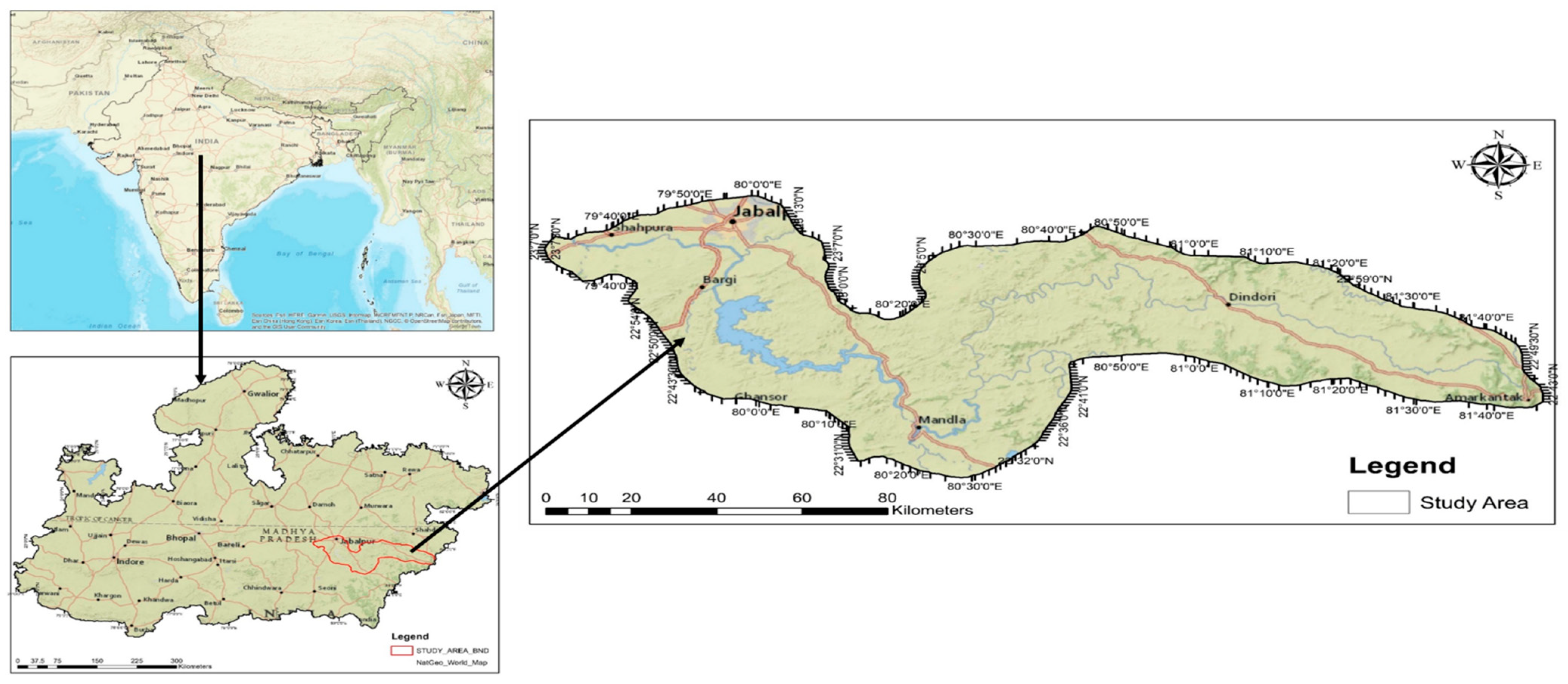
2.1. Study Location

The area’s natural scenery demonstrates its similar geological characteristics. The Vindhyan mountain ranges terminate on the right bank, while the foothills of the Satpura Mountains begin on the left side. This area lies amid a latitude ranging from 22°01′00″ N to 23°01′00″ N and a longitude ranging from 79°0′00″ E to 82°0′00″ E, approximately (Figure 1). The area spans a region of around 9461.09 km² with a mean elevation ranging from 128 to 1048 m above mean sea level. The longer summer months from April to June, the rainy season from July to October, and the winter months from November to February are all a result of the sub-humid tropical monsoon climate. With lows below 6 °C in both April and May, these two months were the hottest and the coldest. There was a temperature range from 16.2 °C to 40.12 °C for the annual mean. The annual precipitation records range from 1360 to 1610 mm. The methodology flowchart delineates the sequential steps involved in the analysis conducted during the ongoing research for the current monitoring and assessment, as shown in Figure 2.

A regression analysis was employed to evaluate the Land Surface Temperature (LST) responses to the Normalized Difference Vegetation Index (NDVI) for both urban and suburban sites, as depicted in Figure 3.

2.2. Data Collection

Satellite data were utilized to look for changes in LULC and NDVI, which are shown in

Table 1. Characteristics of the selected satellite data.

Satellite	Source	Date Acquired	Band	Spectral Range (Wavelength µm)	Spatial Resolution (m)
Landsat 8	USGS	15 August 2022	1	0.43–0.45	30
			2	0.45–0.51	30
			3	0.64–0.67	30
			4	0.53–0.59	30
			5	0.85–0.88	30
			6	1.57–1.65	30
			7	2.11–2.29	30
			8	1.36–1.38	30
			9	0.50–0.68	30
			10 (TRIS 1)	10.60–11.19	100 Resampled to 30
			11 (TRIS 1)	11.50–12.51	100 resampled to 30
Landsat 7	USGS	15 November 2010	1	0.45–0.52	30
			2	0.52–0.60	30
			3	0.63–0.69	30
			4	0.77–0.90	30
			5	1.55–1.75	30
			6	10.40–12.50	60
			7	2.08–2.35	30
			8	0.52–0.90	15
Landsat 5	USGS	15 December 2000	1	0.45–0.52	30
			2	0.52–0.60	30
			3	0.63–0.69	30
			4	0.76–0.90	30
			5	1.55–1.75	30

. Landsat satellite imagery was gathered for this investigation over 3 years: free downloads of the years 2000, 2010, and 2022 were made possible through The National Aeronautics and Space Administration, which is an independent agency of the U.S. website (https://www.usgs.gov), as shown in Table 1. The desired Landsat imagery acquires data in 11 bands, and an image with a band arrangement was obtained through layer stacking. According to Story and Congalton [33], the subsetting procedure was carried out in Arc GIS 10.4, utilizing the image’s extract by mask tools. Based on the field data from the study area for the duration of the years (2000 to 2022), digital LULC classification was performed using a supervised classification technique (maximum likelihood algorithm). Classification accuracy was assessed using a confusion matrix [33]. Error matrices were generated to compare the consistency between the classification results and ground truth data. User, producer, and overall accuracy were computed from the confusion matrix following the methodology outlined in [34]. Additionally, Cohen’s Kappa coefficient was computed to measure the reliability of the classification, as illustrated in

Table 2. Accuracy assessment using confusion matrix generated from 2000 to 2022 (Landsat 8, 7, and 5 images).

User Accuracy (%)						Producer Accuracy (%)					Classification Accuracy	Kappa Statistics
Year	Water Body	Built-Up Land	Agriculture	Forest	Fallow Land	Water Body	Built-Up Land	Agriculture	Forest	Fallow Land
2000	100	85	85	85	80	100	100	73.44	71.44	100	90.00%	0.81
2010	100	75	100	100	85	100	100	100	100	66.68	87.67%	0.75
2022	100	85	100	100	80	100	100	87.34	83.34	100	91%	0.82

[35].

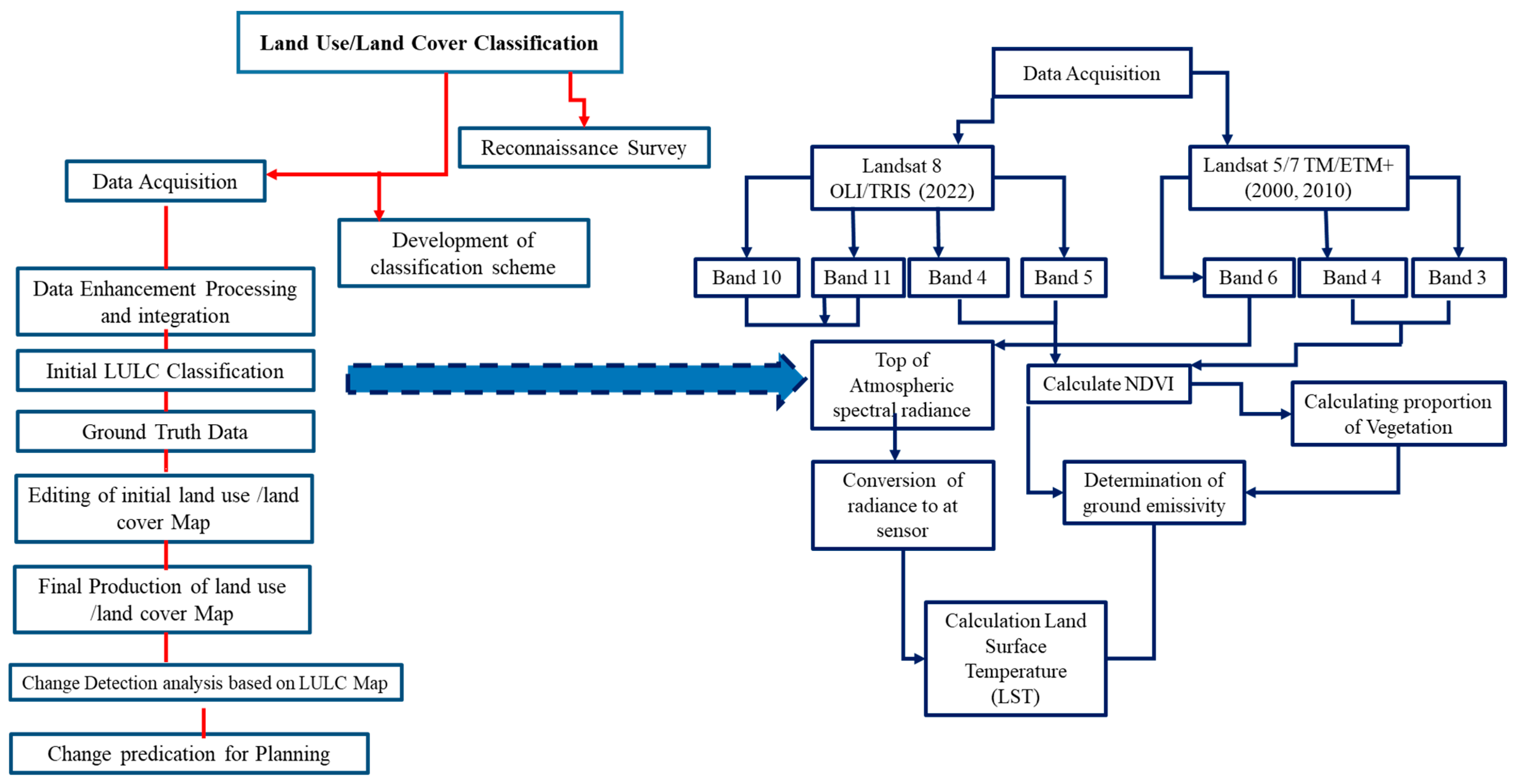
2.3. Methodologies Adopted

2.3.1. LULC Classification

Geometrically corrected Landsat 5 data corresponding to 2000 and 2010 and Landsat 8 data from 2020 were analyzed in the digital environment under the ERDAS IMAGINE 2015 v 15.1 (64-bit) and ArcGIS 10.4 platforms. Both visible and infra-red bands were layer-stacked in ERDAS and projected in the UTM (Universal Transverse Mercator) zone. False Color Composite (FCC) images were generated by combining the bands of 5 or 4, 3, and 2, while image enhancement techniques were employed to increase the contrast of the FCCs. False Color Composites (FCCs) were created from bands 3-2-1 and 4-3-2, respectively (Figure 4), and used as the foundation for the training samples and LULC categorization (Figure 5a). The number of training samples was determined by taking into account the observed abundance and internal variability/homogeneity of each class. With the ESRI ArcGIS training sample management tool, histograms and scatterplots were used to evaluate the reparability of the retrieved training samples. The LULC classifications of water body, built-up land, agriculture, forest, and fallow land were the five main divisions of the research area LULC (

Table 3. Land use land cover in upper catchment area of Narmada River between 2000 and 2022.

S. No.	Classes	2000		2010		2022		Change Detection 2000–2022 (km)2 Increase (+) or Decrease (−)
		Area (km)2	Area (%)	Area (km)2	Area (%)	Area (km)2	Area (%)
1	Water Body	213.71	2.3	289.71	3.06	313.13	3.31	+99.37
2	Built-Up Land	81.85	0.9	124.53	1.31	242.69	2.57	+160.79
3	Agriculture	5607.62	59.3	5693.87	60.18	5651.20	59.73	+43.62
4	Forest	2838.45	30.0	2698.54	28.52	2690.09	28.43	−147.55
5	Fallow Land	719.47	7.6	654.43	6.91	563.98	5.96	−155.68
		9461.09	100.0	9461.09	100	9461.09	100.00

). The MLC algorithm evaluated the probability and cost functions by comparing the spectral signature of each pixel to predefined class signatures [33]. MLC is often used for LULC classification when employing supervised classification techniques. This method is favored due to its ease of implementation, efficiency, and effectiveness, particularly when dealing with a limited number of classes and minimal spectral variability.

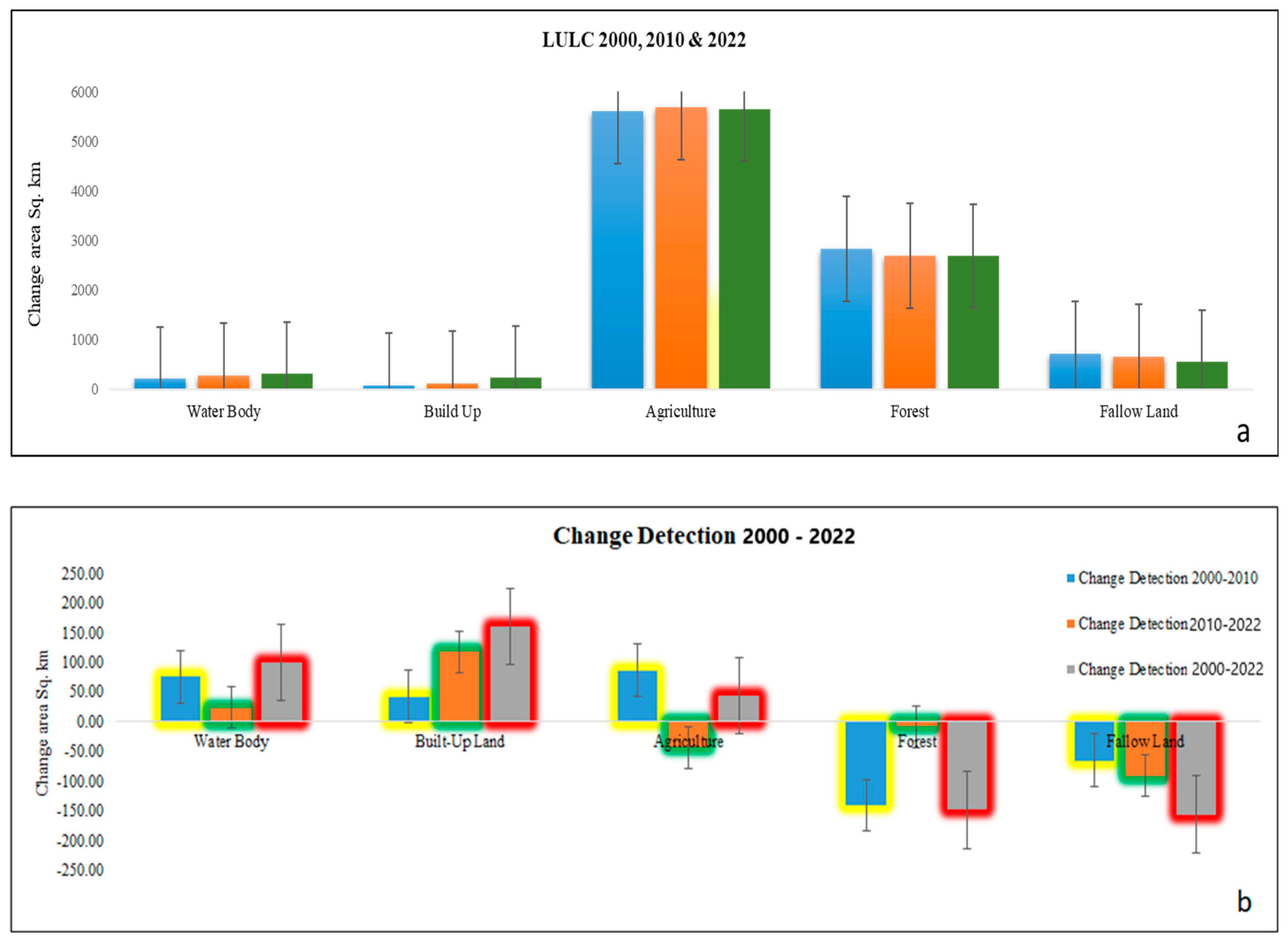
2.3.2. Change Detection Analysis

In the study by Munsi et al. [36], a pixel-by-pixel cross-tabulation analysis was used to construct the change matrix to determine the changes in the land cover classes during the research period from 2000 to 2022. For the years 2000, 2010, and 2022, the LULC change trend, net change, % change, and change rate are all shown, and the times between these three years were computed using the results of the land use/land cover area distribution. (Figure 5b and

Table 4. Cross matrix land use/land cover changes between 2000 and 2022 (Area in km²).

2022
	LULC Change	Water Body		Built-Up Land		Agriculture		Forest		Fallow Land
		Area in	Area in	Area in	Area in	Area in	Area in	Area in	Area in	Area in	Area in
2000		(sq. km)	(%)	(sq. km)	(%)	(sq. km)	(%)	(sq. km)	(%)	(sq. km)	(%)
	Water Body	0	0	18.32	11.39	9.28	21.27	19.97	13.72	14.78	9.49
	Built-Up Land	15.45	15.55	0	0	12.1	27.74	46.89	32.22	39.08	25.10
	Agriculture	34.21	34.43	47.85	29.76	0	0	37.3	25.63	41.83	26.87
	Forest	20.41	20.54	55.7	34.64	15.04	34.48	0	0	59.99	38.53
	Fallow Land	29.3	29.49	38.92	24.21	7.2	16.51	41.39	28.44	0	0
	Total Area	99.37	100	160.79	100	43.62	100	145.55	100	155.68	100

).

$$Change Percentage \left(\mathrm{\%}\right) {\displaystyle \frac{\mathrm{P}\mathrm{r}\mathrm{e}\mathrm{s}\mathrm{e}\mathrm{n}\mathrm{t} \mathrm{L}\mathrm{U}\mathrm{L}\mathrm{C} \mathrm{A}\mathrm{r}\mathrm{e}\mathrm{a}-\mathrm{P}\mathrm{r}\mathrm{e}\mathrm{v}\mathrm{i}\mathrm{o}\mathrm{u}\mathrm{s} \mathrm{L}\mathrm{U}\mathrm{L}\mathrm{C} \mathrm{A}\mathrm{r}\mathrm{e}\mathrm{a}}{\mathrm{P}\mathrm{r}\mathrm{e}\mathrm{v}\mathrm{i}\mathrm{o}\mathrm{u}\mathrm{s} \mathrm{L}\mathrm{U}\mathrm{L}\mathrm{C} \mathrm{A}\mathrm{r}\mathrm{e}\mathrm{a}}}\times 100$$

(1)

2.3.3. Conversion of a Digital Number to Visibility LST Using Landsat 5 Thematic Mapper

The LST is computed by translating the digital number for the TM sensor into radiance. The TM sensor’s radiance value was converted into an integer using the metadata file’s equation.

$$L\lambda ={\displaystyle \frac{\left(\mathrm{L}\mathrm{M}\mathrm{A}\mathrm{X}\mathsf{\lambda }-\mathrm{L}\mathrm{M}\mathrm{I}\mathrm{N}\mathsf{\lambda }\right)}{\left(\mathrm{Q}\mathrm{C}\mathrm{A}\mathrm{L}\mathrm{M}\mathrm{A}\mathrm{X}-\mathrm{Q}\mathrm{C}\mathrm{A}\mathrm{L}\mathrm{M}\mathrm{I}\mathrm{N}\right)}}\left(\mathrm{Q}\mathrm{C}\mathrm{A}\mathrm{L}-\mathrm{Q}\mathrm{C}\mathrm{A}\mathrm{L}\mathrm{M}\mathrm{I}\mathrm{N}\right)+\mathrm{L}\mathrm{M}\mathrm{I}\mathrm{N}\mathsf{\lambda }$$

(2)

where Lλ denotes the watts of spectral radiation at the sensor’s aperture (m² × ster × µm), QCALMIN is the smallest quantized calibrated pixel value in DN, and LMINλ is the watts-scaled spectral radiance to QCALMIN/(m² × ster × µm); LMAXλ is equal to the spectral radiance that scales to QCALMAX in watts per (m² × ster × m), QCALMIN is the smallest quantized calibrated pixel value (LMINλ in DN), and QCALMAX is the highest quantized calibrated pixel value possible in DN = 255.

The next step is to determine the land surface temperature (LST), which is the effective satellite-visualized temperature of the Earth’s atmosphere visual system in the case of Landsat 5–7 photos [37]. Converting from Kelvin to Celsius requires adding −273.15. The equation is:

$$T{\displaystyle \frac{K2}{In\frac{k1}{L\lambda }+1}}-273.152$$

(3)

where T indicates Kelvin-based heat, K2 is the Metadata fill calibrating regular 2, k1 is the Metadata fill calibrating regular 1, and L is the spectral radiance in watts per (m² × ster × m).

The process is more complicated when it comes to Landsat 8 scenes. According to the 2019 LANDSAT 8 (L8) data user’s manual, the first step is to convert the digital values into radiance units using the following equation:

$$\left(\mathrm{L}\mathsf{\lambda }=\mathrm{M}\mathrm{L}\mathrm{Q}\mathrm{c}\mathrm{a}\mathrm{l}+\mathrm{A}\mathrm{L}\right)$$

(4)

where Lλ is (W/(m² × ster × m)) spectra radiance, ML is the additive rescaling factor (RADIANCE_ADD_BAND_x, where x is the band number that is particular to a given band), AL is a band-specific additive rescaling factor (RADIANCE_ADD_BAND_x, where x is the band number) from the information, and Qcal is standard product pixels that have been quantized and calibrated.

2.3.4. Radiance to Satellite Temperature Conversion

The NASA Earth data search portal is utilized to obtain data for the LST’s monthly MODIS daylight terrestrial emissivity from 2000 to 2022 to calculate the average change. The Kelvin temperature of a satellite is calculated using the computed radiation value from the TM sensor and the equation below.

The thermal constants provided in the metadata file are also used to change the OLI/TIRS thermal band data from spectral radiance (obtained from Equation (2)) to the top of the atmospheric brightness temperature: the average of both bands (bands 10 and 11) at the satellite temperature is calculated for this study.

2.3.5. Obtaining the Ground Surface’s Emissivity

The retrieval of land surface emissivity occurs following the calculation of NDVI. Following is a formula for calculating the land surface emissivity of the two sensor images.

$$e=0.004PV+0.986$$

(5)

where e is the land surface emissivity and Pv is the proportion of vegetation,

$$PV={\displaystyle \frac{NDVI-NDVImin}{\left(NDVImax-NDVImin\right)}}2$$

(6)

where NDVI min is the lowest value of the NDVI and NDVI max is the highest value of the NDVI.

Land Surface Temperature (LST):

$$LST={\displaystyle \frac{BT}{1}}+W{\displaystyle \frac{BT}{P}}\times Ln\left(e\right)$$

(7)

where BT is the satellite temperature and w is the wavelength of emitted radiance (0.00115).

$$\mathrm{P}={\displaystyle \frac{\mathrm{h}\times }{\mathrm{s}}}(1.438\times {10}^{-2} \mathrm{m} \mathrm{K})$$

where h is Planck’s constant (6.26 × 10⁻³⁴ J s), s is the Boltzmann constant (1.38 × 10⁻²³ J /K), and c is the velocity of light (2.998 × 10⁻⁸ m/s and P = 14,380.

By averaging two thermal bands from Landsat 8 OLI/TIRS, bands 10 and 11, it is possible to determine the land surface temperature for 2022.

2.3.6. Normalized Difference Vegetation Index (NDVI)

Using the NDVI, the land surface emissivity for both research years is calculated. This involves calculating the NDVI for the Landsat TM, 2000, 2010, and 2022 (Figure 3). Consequently, the NDVI is determined using the following formula.

$$\mathrm{N}\mathrm{D}\mathrm{V}\mathrm{I} \mathrm{T}\mathrm{M}={\displaystyle \frac{\mathrm{B}\mathrm{a}\mathrm{n}\mathrm{d} 4-\mathrm{B}\mathrm{a}\mathrm{n}\mathrm{d} 3}{\mathrm{B}\mathrm{a}\mathrm{n}\mathrm{d} 4+\mathrm{B}\mathrm{a}\mathrm{n}\mathrm{d} 3}}$$

(8)

Band 4 is near-infrared (NIR) and band 3 is red.

$$\mathrm{N}\mathrm{D}\mathrm{V}\mathrm{I} \mathrm{L}\mathrm{a}\mathrm{n}\mathrm{d}\mathrm{s}\mathrm{a}\mathrm{t} 8={\displaystyle \frac{\mathrm{B}\mathrm{a}\mathrm{n}\mathrm{d} 5-\mathrm{B}\mathrm{a}\mathrm{n}\mathrm{d} 4}{\mathrm{B}\mathrm{a}\mathrm{n}\mathrm{d} 5+\mathrm{B}\mathrm{a}\mathrm{n}\mathrm{d} 4}}$$

(9)

where band 5 is near-infrared and band 4 is red.

2.3.7. NDVI Estimate for Measuring Land Degradation

To identify and measure the presence of living, green vegetation, the NDVI analyzes the reflected light in the NIR and visible ranges. Simply described, the NDVI is a statistic that assesses each pixel’s level of greenness and plant health in a satellite image. With the expanded use of remotely sensed data received from satellite data, scientists and researchers have started to employ the NDVI in their studies. The NDVI measures biomass and greenness [6]. The range of the NDVI is from +1 to −1. Negative numbers indicate non-vegetated regions, whilst positive values aid in identifying vegetated and non-vegetated areas [6]. The NIR band plus the RED band divided by the NIR band equals the NDVI. Reflectance from Landsat’s visible red 4 and NIR band 5 (0.84–0.89 m and 0.64–0.67 m) wave bands is radiated in the NIR band and the RED bands.

2.3.8. Drivers of Land Degradation and Land Degradation Vulnerability

The Land Degradation Vulnerability Index (LDVI) model was developed using all possible combinations of the priority classes in order to evaluate the overall effect of environmental factors on land degradation at the ground level. The criteria variables of land degradation were integrated with ArcGIS using the weighted overlay tool under the spatial analysis scheme, and are depicted in the Supplementary Tables S1 and S2. When iterating the model through weighted overlay analysis, the cell values of the inputs, corresponding to the 16 criteria variables, were multiplied by the weights obtained from the MVA analysis [33]. The individual cell values were added together to produce the final output raster model, where higher values indicate a high vulnerability to land degradation and lower values are indicative of a low vulnerability to degradation. The model divided the research region into five groups based on its sensitivity to land degradation: very low, low, moderate, high, and very high.

$$\mathit{LDVI}={\sum }_{i=1}^{n=7}DFi\times Wi$$

(10)

where n is the number of factors, DF is the defining factor, Wi is the weight of the determining factor, and (criterion = 7) is the overlapping maps that produced the LDVI map. The five land degradation vulnerability classes—very high vulnerability (>7), high vulnerability (5 to ≤7), moderate vulnerability (3 to ≤5), low vulnerability (1 to ≤3), and very low vulnerability (<1)—were defined.

3. Results and Discussion

3.1. Evaluation of the LULC Classification’s Accuracy

This study employed temporal satellite imagery from 2000 to 2022 to investigate the relationship between LST and LULC changes in the study area. To provide a trustworthy LULC classification result, a classification accuracy evaluation is crucial. In the current investigation, the confusion matrix’s outcome, which evaluated the LULC classification’s accuracy, is shown in Table 2. With Kappa values of 0.81, 0.75, and 0.82, the overall correctness of each year’s grouped LULC categories (2000, 2010, and 2022) was, respectively, 90.0%, 87.67%, and 91%. The most accurately categorized LULC, with complete producer and user correctness reported for every year, was water bodies, as seen in the producer and user accuracy data. The forest class, where the categorization likewise performed well, had user and producer accuracies of up to 80% and 100%, respectively. The built-up land, fallow land, and agriculture groups all yielded relatively accurate results.

The percentage of the map that is accurately categorized from both the user’s and producer’s perspectives is measured by the user and producer accuracy. The Kappa coefficient represents the proportionate improvement by the classifier over a simple random assignment to classes [38,39]. The classification accuracies obtained in our study, with most classes exceeding a 90% accuracy using the MLA, were precise and fell within the acceptable limits for accurate classification [40]. Typically, the classification accuracy greater than 80%, along with Kappa statistics above 0.8, considered to be sufficient for accurately characterizing landscapes in heterogeneous environments [41]. Moreover, our results align with the established benchmarks for classification accuracy [10,13,15].

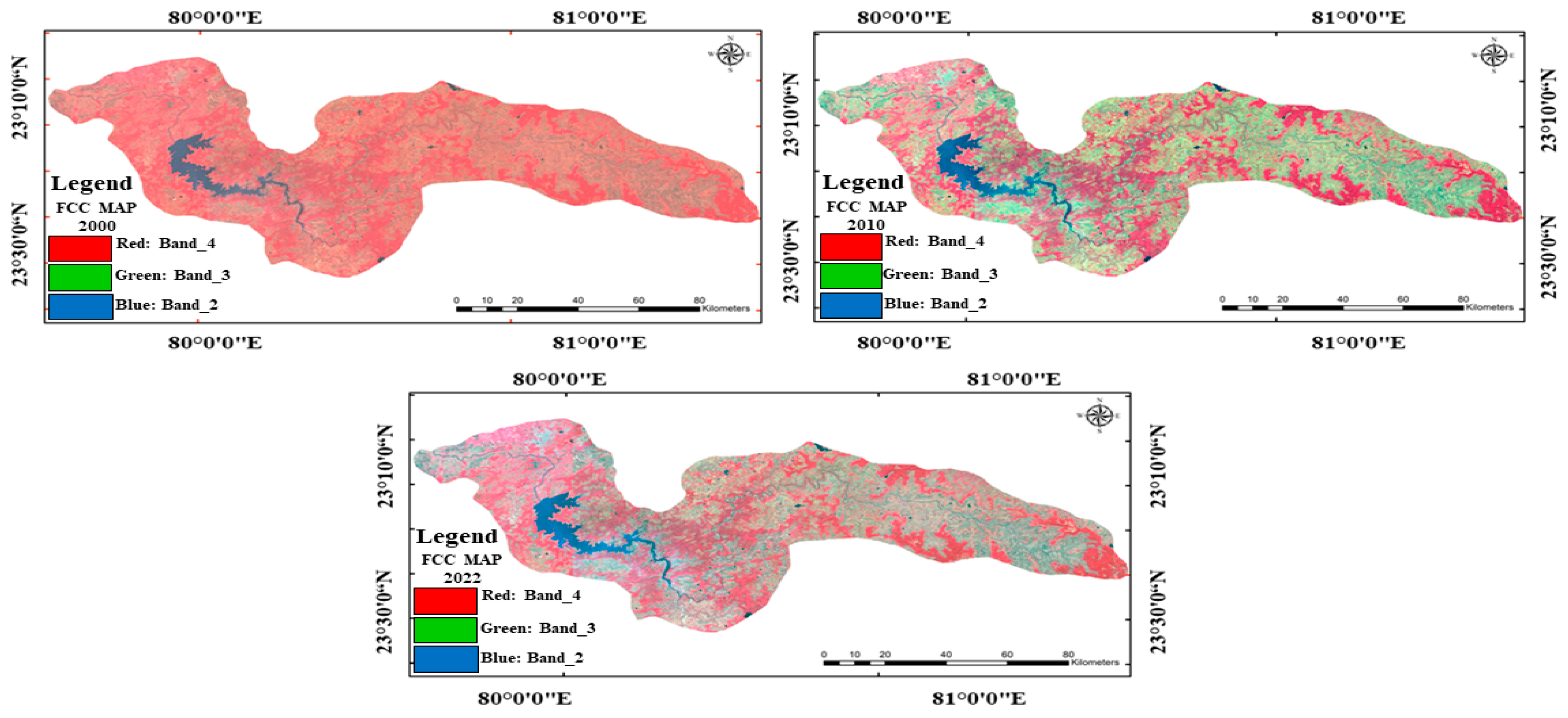
3.2. The LULC’s Spatial and Temporal Pattern

The spatial distribution patterns of land cover and vegetation, along with the accuracy levels achieved with the application of ML algorithms in the upper catchment of the Narmada landscape of the study area, are summarized in Table 2 and Figure 4. Five types of land use classes were identified: (1) forest, (2) agriculture, (3) fallow land, (4) built-up areas, and (5) water bodies. A land use analysis revealed that the study area is spread over 9461.09 km², with agriculture fields (59.3%), forests (30%), and fallow land (7.6%) initially being more or less in equal proportions in the year 2000, while water bodies (2.3%) and built-up (0.9%) areas were restricted to a small region (Table 3). Each classed region is summarized in Table 3, as well as the changes in the area for the years of 2000, 2010, and 2022. Figure 6a provides a class-based visual depiction of the expanded region and the geographical distribution of the categorized LULC classes. The Narmada River and its tributaries, as well as the urban perimeter (outside of built-up regions and fallow land), were the main locations for land in the forest class. Most of the agricultural LULC class was found in the area between forested and built-up land. Regardless of the year, agriculture had the highest area coverage, accounting for 5607.62 km² (59.63 (59.3%) in 2000, 5693.87 km² (60.18%) in 2010, and 5651.20 km² (59.73%) in 2022. The forest LULC class was the second-most prominent LULC class in 2000, making up approximately 2838 km² (30%) of the land area. However, this proportion gradually declined, falling to around 2690.09 km² (28.43%) in 2022 (Figure 6a). During the time frame of the study, the water bodies’ locations remained largely consistent. The built-up LULC class, making up the city’s center, experienced substantial growth. According to Figure 5b and Figure 6a, the built-up land LULC class expanded steadily but gradually between 2000 and 2022. It is clear that the built-up land space that makes up the urban landscape has grown in size with each passing year by comparing the locations of the different LULC categories across all years (Figure 6b).

Given the evident rise in urban land use, which is represented in the built-up land and fallow land LULC classes and includes a sharp decline in the forest LULC, the effects of urbanization may be blamed for the change in the total LULC in the study region. Urbanization processes frequently impose strain on the available undeveloped lands, which are generally agricultural regions and the expanding areas next to city centers [40]. Despite the losses in forests and water bodies in the study area, agriculture remained more or less stable, only increasing by 1.01% in 22 years, while drastic changes in other land use classes were observed between 2000 and 2010 and also between 2010 and 2022. However, the rates of LULCC and land degradation were found to be higher from 2000 to 2010, while there was a rapid increase in built-up areas between 2010 and 2022 (Table 4). The built-up area was increased by almost 300% with the conversion of parts of agriculture areas, fallow lands, wooded forest lands, and water bodies. The main drivers of deforestation and degradation are the over-exploitation of land for unproductive uses, the conversion of forest lands into illegal agriculture fields, and inappropriate restoration plans in disturbed areas. ML algorithms are frequently employed for hyperspectral image classification and object detection in remote sensing data analyses [41,42]. However, they have also demonstrated a promising performance in the classification of multispectral imagery [19]. Numerous studies have overwhelmingly reported that anthropogenic activities are responsible for unwarranted land use changes and the conversion of dense forests into open forests, whereas agriculture encroachments are largely responsible for forest degradation [26,41,42].

Quantifying land degradation in the upper catchment of the Narmada River using Landsat imagery necessitates a comprehensive understanding of forest dynamics in terms of both land cover and land use. Forest land cover includes critical attributes such as canopy density, phenology, and canopy height, each of which can fluctuate due to both natural and anthropogenic influences. Dense forests exhibit greater canopy cover, while signs of degradation can manifest through reductions in forest density and canopy cover. Phenological variations, observable through seasonal changes, provide insights into vegetation health, with declines in canopy height often being indicative of deforestation and associated land degradation processes. From a land use perspective, forests within the catchment serve multiple functions, including timber production, conservation, grazing, and agroforestry. Timber extraction, particularly through clear-cutting or selective logging, is detectable via decreases in vegetation indices such as the NDVI, indicating forest degradation. Conservation areas typically maintain forest cover as stable or improve it, unless disrupted by human encroachment. Overgrazing, which can result in soil compaction and hinder forest regeneration, can be identified through changes in land cover types captured by satellite imagery. Forest management practices within the catchment range from natural, unmanaged forests that deliver essential ecosystem services to managed plantations and selectively logged areas, which are at risk of degradation if not managed sustainably. By leveraging Landsat imagery to monitor shifts in forest land cover and land use, this study aims to quantify the extent of forest degradation and evaluate its underlying drivers. Such an analysis is crucial for understanding the broader environmental impacts affecting the upper Narmada catchment. Given that forests in this region often function as common property resources (CPRs), they are particularly vulnerable to anthropogenic pressures. Integrating scientific research with decision support systems and fostering social engagement are essential for addressing conservation challenges and promoting sustainable forest management.

Cross-tabulation matrices depicting the transitions in land use changes from one category to another category between 2000 and 2022 are presented in Table 4. The analysis of the change matrix revealed that, in total, approximately 6.5% of land underwent alterations, either in a positive or negative direction, over the past two decades (2000–2022). Out of the 2838.45 km² of forest land in 2000, only 2690.09 km² remained as forest land in 2022, whereas 5% was transformed into other classes, about 46.89 km² area was converted into built-up area, 41.39 km² into fallow land, 37.3 km² into agriculture, and 19.97 km² into water bodies. However, 43.62 km² of the area added to agriculture was mainly from forests (15.04 km²), built-up areas (12.1 km²), water bodies (9.28 km²), and fallow land (7.2 km²), thus, only 0.43% of land was added between 2000 and 2022.

The substantial impact of human-induced disruptions, such as settlements, infrastructure development, road construction, and mining, led to a significant decline in forest cover and an appreciable increase in built-up area and agricultural land near the Narmada basin. Out of the total area of 9461.09 km², fallow land was about 719.47 km² in 2000, out of which, about 563.98 km² was retained under this class in 2022 and almost 155.68 km² was transformed into forests (59.99 km²), agriculture fields (41.83 km²), built-up areas (39.08 km²), and water bodies (14.78 km²). Inevitably, it was noticed that the built-up area class exponentially increased from 81.85 km² to 242.69 km² over the last 22 years, while major areas from the forest and agriculture classes (103.55 km²) were added to build up area. Forest and fallow land shrunk significantly, accounting for 3.21% of the expanse of built-up areas, water bodies, and agriculture, which resulted in the expansion of degraded river basins between 2000 and 2022. The built-up area was increased by almost 1.67% with the conversion of forests, agriculture fields, and fallow lands (Table 4).

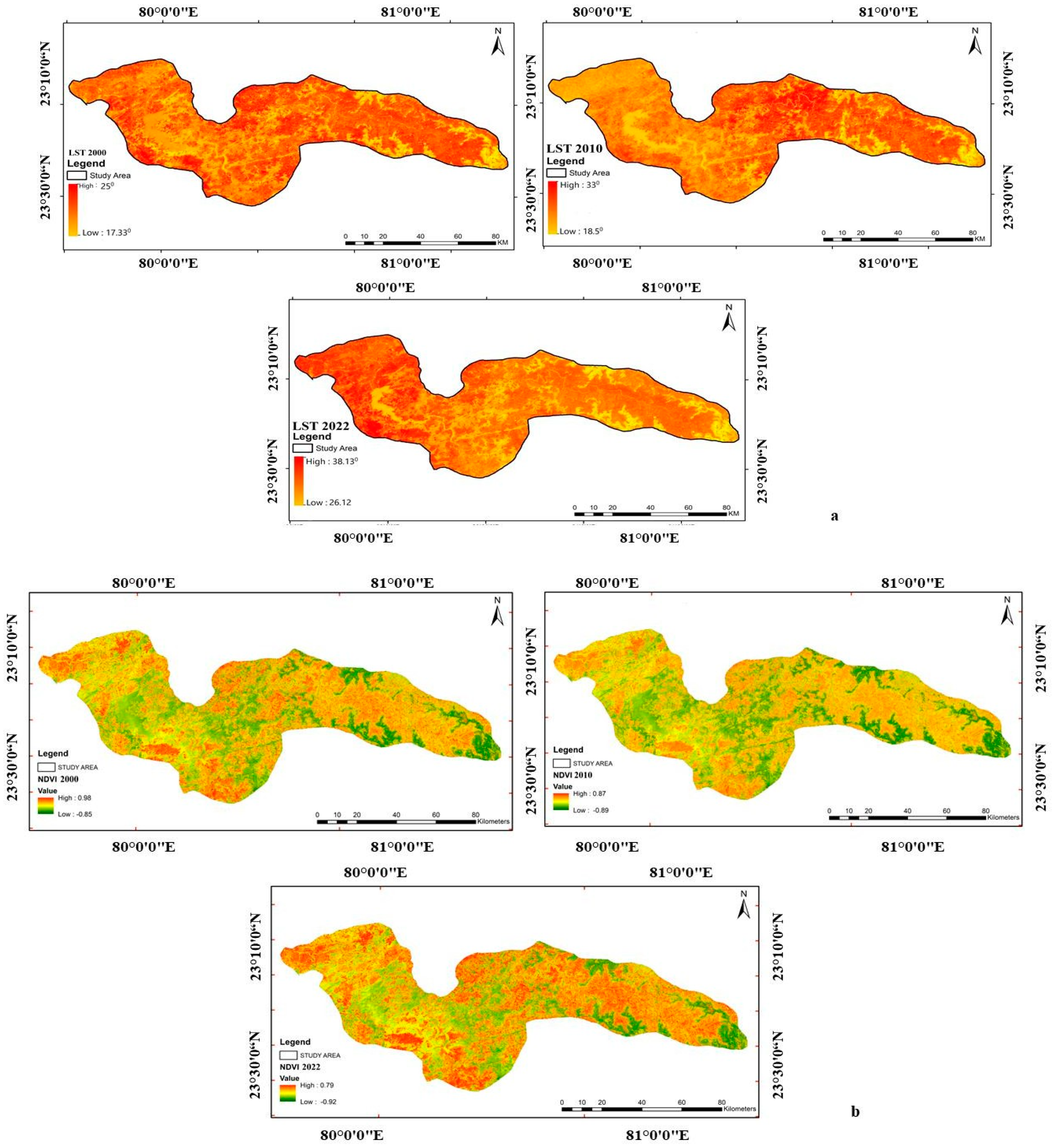
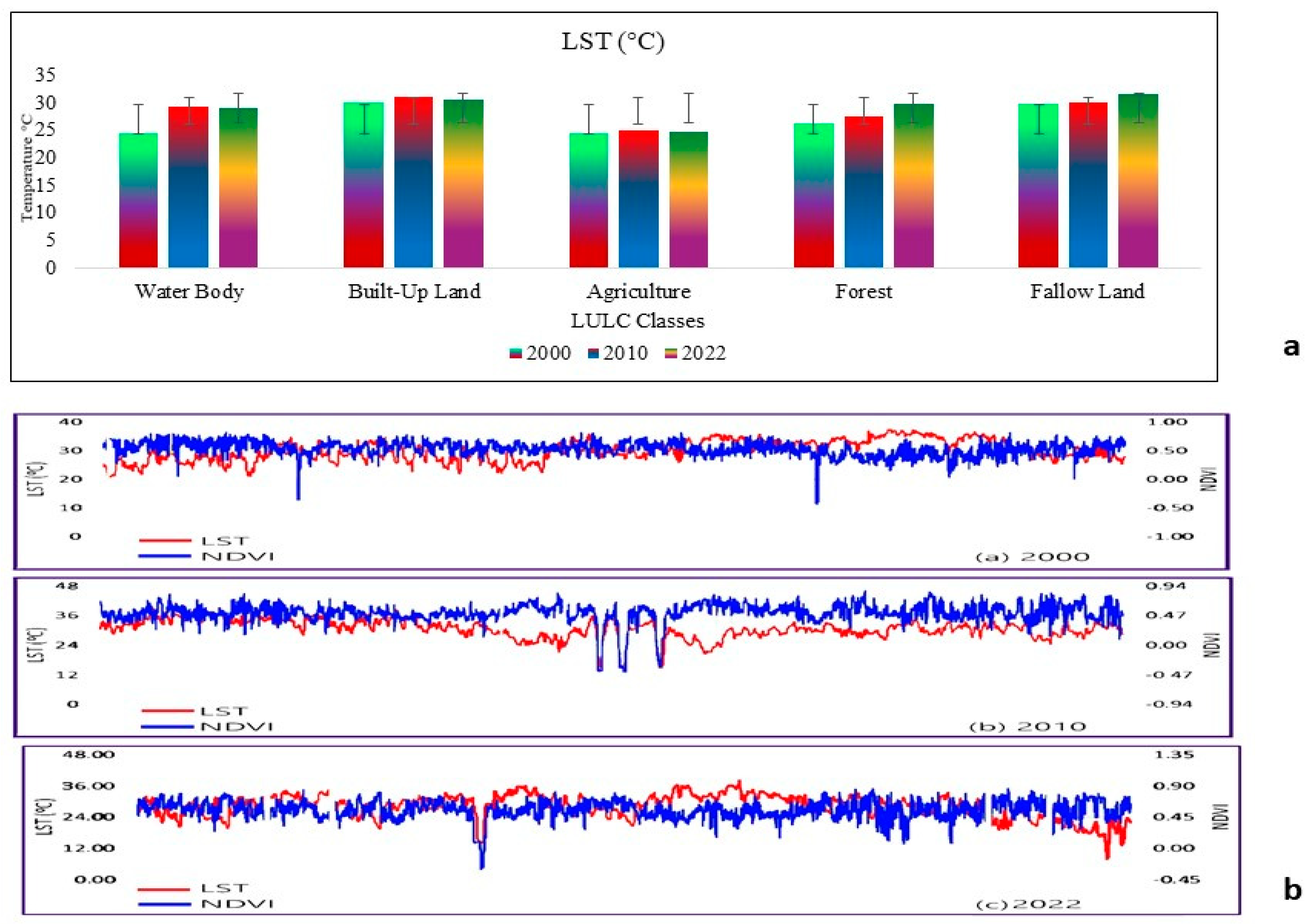
3.3. Land Surface Temperature Variation between 2000 and 2022

Based on seasonal fluctuations, the monthly statistics for terrestrial emissivity are categorized. Four main seasons have an impact on the research area: winter, summer, southwest monsoon, and northeast monsoon. MODIS data are used to construct surface temperature land maps for the years from 2000 to 2022, which are seen in Figure 7a based on these seasonal factors.

Table 5. Validation of remotely sensed LST.

Year	2000		2010		2022
Source of estimated/recorded LST	Maximum	Minimum	Maximum	Minimum	Maximum	Minimum
Remotely sensed estimated LST (°C)	25.32	17.42	33	18.50	38.13	26.12
IMD-recorded LST (°C)	28.2	21.01	29.61	22.22	34.01	24.91
Deviation (°C)	2.97	3.08	−3.88	3.7	−4.75	−1.76
Deviation (%)	10.30	16.92	−13.15	16.67	−14.08	−7.02

lists the seasonal LSTs that were derived from the MODIS data. Temperature ranging between 23 °C and 17.33 °C, 33 °C and 18.5 °C, and 38.13 °C and 26.12 °C, respectively, were recorded in 2000, 2010, and 2022. The LST during the winter time recorded in 2000 was 25 °C, while it changed to 31.29 °C in 2022. During the designated timeline for the study, the maximum temperature recorded was 32.5 °C in 2010 and the minimum temperature was 16.32 °C in 2000. From 2000 to 2022, the summer time mean temperature from 24.89 °C to 36.59 °C, where the maximum recorded temperature was 32.25 °C in 2010 and the minimum was 22.15 °C in 2022. The average temperature during the SW monsoon season was 22.89 °C in 2000 and 32.3 °C in 2022. In the year 2000, the maximum and minimum readings were 22.89 °C and 15.3 °C. The mean temperature decreased between 2000 (24.15 °C) and 2022 (30.15 °C) during the NE monsoon season. The peak temperature for this season was 29.89 °C in 2010, while 22.51 °C was recorded for the minimum in both those years. Figure 7a displays a graph representing the typical seasonal changes in the LST.

3.4. Evaluation of the LST Estimate

The spatiotemporal distribution of the LST was tracked using an accurate and well-established methodology, yet it still is not without small errors. It is ideal to have a clear sky without any clouds in the study area to obtain an entirely accurate photo to determine the LST. Even if the cloud cover was less than ten percent, it was not zero, therefore, the data collected from the field were not the same [43]. Knowledge of the LST distribution in any area may be biased as a result of such a situation. For 2000, 2010, and 2022 in the study region, the maximum and minimum temperature data were gathered from the meteorological stations of the Indian Meteorological Department (IMD) to validate the predicted LST and a deviation was determined (Table 5). A positive deviation (PD) shows a lower estimated LST, while a negative deviation (ND) indicates estimated values that are higher than the BMD-documented temperature. With extreme LSTs of (2.97) for 2000 and (1.76) for 2022, the highest PD and ND were determined. The greatest average PD (+1.8) and ND (1.23) were discovered for the years 2010 and 2021, respectively.

In 2000, 9.73%, 27.10%, and 30.39% of the study area were, respectively, in the 18–25–29 °C, 19–25–29 °C, and 25–29 °C temperature ranges, but in 2021, more than 75% of the study area was in the 30–31 °C (31.51%), 32–33 °C (21.38%), and 34–37 °C (18.85%) temperature ranges. The temperature in the research region grew progressively between 2000 and 2010, with increases of 27.10% and 30.39% in the temperature ranges from 19 to 29 °C and from 30 to 31 °C, respectively, with a significant rise of 9.73% in the temperature range of 19 °C. In addition, 12.24% was further added between 2010 and 2022. The entire past three-decade scenario (2000–2022) revealed a large decrease in temperatures between 19 °C and 30 °C (18.40%), 26 °C and 29 °C (31.37%), and 30 °C and 31 °C (9.81%), as well as an immediate increase in temperatures between 32 °C and 33 °C (17.52%), 34 °C and 35 °C (3.61%), 36 °C and 37 °C (18.68%), and 38 °C (Table 5).

3.5. Spatial Trend between LST, NDVI, and LULC Relationship

The spatial aggregation of LULC has been shown to affect the LST and surface temperature in general, according to studies. Zhibin et al. [44] pointed out that, for instance, spatially aggregated vegetative land cover, which is known to be generally inversely associated with LST, can achieve a considerable reduction in LST, while fragmented LULC has fewer effects on LST. Natural factors that affect land surface temperature include changes in land use and land cover. Places categorized as built-up land, forest, fallow land, agricultural land, and water bodies were shown to have high temperatures during the past two decades (Figure 7a). The average LST measurements for agricultural land were recorded at 24.46 °C in 2000, 24.87 °C in 2010, and 24.58 °C in 2022. Agricultural land’s temperature dropped by 0.29 °C over the period. Built-up land was recorded as having an average temperature of 30.11 °C in 2000, 30.94 °C in 2010, and 30.58 °C in 2022. LST in this area decreased by 0.47 °C, despite the area increasing. In 2000, the average temperature recorded for fallow land was 29.65 °C; 30.06 °C in 2010; and 31.6 °C in 2022. The average temperature of fallow land appeared rise by 0.41 °C between 2000 and 2010, while an additional increase of 1.54 °C was recorded between the years 2010 and 2022 and an overall decrease of 1.95 °C was recorded between 2000 and 2022. The mean temperatures in the years 2000, 2010, and 2022 for water bodies were recorded as 24.48 °C, 29.18 °C, and 28.9 °C, respectively. From 2000 to 2022, the temperature declined by 4.7 °C, but the area also shrank. In the years 2000, 2010, and 2022, the average temperatures in forests were recorded as 26.32 °C, 27.44 °C, and 29.6°C. From 2000 to 2022, the temperature dropped by 3.28 °C, but the area shrunk as well. While built-up area and the agricultural land had high LSTs, water bodies were seen to have low temperature levels.

Even though built-up land, fallow land, and agricultural land had the highest LSTs among the categorized groups [11,45,46], comparing the LULC in Figure 7a,b, it can be revealed the built-up area and fallow lands LULC categories had the greatest mean LSTs and lowest NDVIs in all the years considered, and that the geographical distribution of LST and NDVI reflected the pattern of LULC in the research region. Every year’s NDVI followed the same pattern as the LST. The NDVI values in built-up land regions were generally low, whereas those in the forest LULC class were rather higher (Figure 7b).

3.6. Land Degradation Vulnerability Index (LDVI) Analysis

The LDVI modeling framework offered a chance to spatially quantify the overall impacts of several environmental, social, and economic aspects on land. Decreasing at the local level, as determined from the study site (Figure 8,

Table 6. Spatial extent of land degradation vulnerability classes in the study area.

LDVI Classes	Area (km2) 2022	Percentage
Very Low Vulnerability	2289.25	24.20
Low Vulnerability	1319.65	13.95
Moderate Vulnerability	1213.22	12.82
High Vulnerability	1134.1	11.99
Very High Vulnerability	2949.05	31.17
Built up	242.69	2.57
Water Bodies/Drainage	313.13	3.31
Total	9461.09	100.00

), 43.16% of the research area (4128.15 km²) had LDVI values that were extremely high or high, indicating a significant sensitivity to various types of land degradation. In order to reduce the susceptibility of land-to-land degradation, these locations (included in Table 6) need urgent improvements to their socio-economic and biophysical contexts. A total of 38.15% of the area (or 3608.9 km²) had LDVI values that were low or very low, indicating that these regions are not as vulnerable to land degradation as others. However, 12.82% of the area (or 1213.22 km²) had a moderate LDVI, indicating a limited susceptibility to several land degradation processes.

In this research, water bodies and built-up areas, totaling around 5.88% of the area, exhibited no sign of land degradation, as depicted in Figure 8. Previous studies have also proved that the NDVI is useful for detecting plant stress, depending on the nature and extent of land degradation. The application of the AHP-based Multi-Criteria Analysis (MCA) procedure is useful in assessing land degradation, which was corroborated by reports from previous studies [9,47,48,49,50,51]. Pandey et al. [48] quantified the impact of mining on land degradation vulnerability using the MCA tool, considering the major determinants, viz., biophysical, topographic, and soil/edaphic factors, and found that NDVI and topographic conditions are strong determinants that affect the vulnerability of soil degradation. One of the major influencing factors affecting the process of land degradation is the variation in climatic conditions (i.e., soil index, climate index, terrain index, and land utilization index are depicted in SF1). Our findings using the MCA were almost in agreement with the results from previous studies [52,53,54]. MCA analysis enables sorting out the critical elements affecting the LDVI and helps in adopting a triage approach before embarking on the decision-making process, while allocating scarce resources and rationally balancing trade-offs while implementing restoration plans in the Narmada River landscape [55].

3.7. Future Perspective: An Integrated Narmada River Basin Restoration Approach for Degraded Land Reclamation

The primary objective of this investigation is to comprehensively analyze the root causes and consequences of land degradation and their evolution over the span of two decades in the upper Narmada River catchment area. The investigation aims to gain profound insights into the factors contributing to river degradation, its associated ecosystems, and the biodiversity within and around the river. River restoration, in this context, is not merely about returning the river to its original state, but rather focuses on enabling the river to effectively manage and restore its natural processes and biological diversity, thereby maximizing the benefits for both human populations and wildlife [55]. Firstly, it seeks to restore the natural meandering course of the river, which fosters habitat diversity and biological richness. This can be achieved by either reverting to the old river route or constructing an alternative route if the original channel is inaccessible or unidentified. Secondly, it emphasizes the restoration of floodplain connectivity and the formation of wetlands, recognizing that these habitats are often disrupted due to land reclamation for agriculture, development, or housing. In cases where floodplain restoration is not feasible due to urbanization, in-stream enhancement becomes a viable alternative, involving various techniques tailored to the catchment area’s restoration needs. Lastly, removing or bypassing barriers such as barrages and dams are crucial, as these structures impede the free movement of biological diversity and sediment transport across the river catchment, thereby altering the natural habitat of both aquatic and terrestrial ecosystems and leading to significant landscape changes over time [19].

Analyzing the data on land use and land change indicates that the gradual shifts observed in the upper Narmada River catchment over the past two decades have been driven by overarching factors such as urbanization, infrastructure development, economic growth, population increase, and changing climatic conditions. The scientific findings of this study, coupled with GIS models, serve as robust sources of information, providing a solid scientific foundation for policy formulation concerning river restoration and landscape conservation in the area. However, the effective implementation of river restoration initiatives requires seamless collaboration among different government departments and ministries, including urban planning, pollution control, forest management, municipal corporations, land revenue, public works, and others. Overcoming challenges related to jurisdictional mandates and expertise gaps is crucial, necessitating the establishment of foundational ethical principles that can be uniformly applied across all branches to ensure holistic river management. A competent governing body with jurisdictional competence and a lawful mandate plays a pivotal role in fostering harmony among stakeholders and coordinating interdisciplinary involvement across various departments and ministries, alongside active community participation throughout the catchment area. The current land degradation in the Narmada basin is driven by various factors, including agricultural practices, urbanization, deforestation, and climate change. Expanding deforestation and agricultural activities, particularly in hilly areas, has accelerated soil erosion, resulting in a reduced soil fertility and declining crop yields. Additionally, rapid urban growth and infrastructure development have transformed agricultural land and natural habitats into urban areas, thereby increasing pressure on the region’s remaining land resources [19]. Addressing land degradation in the Narmada basin necessities the implementation of integrated management strategies that focus on sustainable land use, reforestation, improved agricultural practices, and community engagement. The restoration of degraded lands and conservation initiatives are crucial for mitigating ongoing degradation and fostering ecological resilience.

4. Conclusions

The study revealed extensive land use and land cover (LULC) changes, resulting in unprecedented land degradation and ecological disruption in the upper Narmada River catchment area, India. The vulnerability to land degradation in this region is exacerbated by the complex interplay of undulating topography, shifting soil characteristics, climatic variations, evolving agricultural practices, infrastructural developments, and shifting livelihoods. The Normalized Difference Vegetation Index (NDVI) and Land Surface Temperature (LST) were identified as key indicators for assessing land degradation vulnerability. The study highlighted the intricate relationships between LULC types, land surface attributes, and LST patterns, demonstrating diverse impacts across different land categories. An inverse correlation between LST and vegetation abundance was observed across all LULC types in the Narmada River basin, with urban areas and certain forested regions showing a heightened sensitivity of LST to NDVI variations. This underscores the potential of expanding vegetation covers to mitigate urban heat island effects in these areas. The study also distinguished between land use/land cover conversion and modification, highlighting that the latter often has less pronounced impacts on land cover attributes. While conventional approaches emphasize land preservation as a key strategy for combating land degradation, this study critically analyzed the efficacy of ongoing land convergence initiatives and their varying outcomes across different regions.

The use of Geographic Information Systems (GISs) was instrumental in the decision-making processes, facilitating the rapid identification of problems, criteria selection, and informed judgments regarding land vulnerability. The results underscored the significance of the NDVI, along with rainfall and temperature, in determining land degradation susceptibility. Approximately half of the study area exhibited a “high vulnerability” on the Land Degradation Vulnerability Index (LDVI) map, necessitating targeted restoration efforts and site-specific interventions. Achieving the Sustainable Development Goal (SDG) of zero net land degradation by 2030 hinges on the effective implementation of comprehensive measures to reverse ongoing land degradation at a localized level. The study advocated for the integration of Multi-criteria Analysis (MCA) with GISs to generate LDVI maps and prioritize zones for reclamation and revegetation, thereby fostering eco-restoration initiatives.

References

1. UNCCD. Towards a Land Degradation Neutral World: A Sustainable Development Priority. Available online: https://www.unccd.int/land-and-life/land-degradation-neutrality/overview (accessed on 26 August 2024).
2. Sims, N.C.; Barger, N.N.; Metternicht, G.I.; England, J.R. A land degradation interpretation matrix for reporting on UN SDG indicator 15.3. 1 and land degradation neutrality. Environ. Sci. Policy 2020, 114, 1–6. [Google Scholar] [CrossRef]
3. Stavi, I.; Lal, R. Achieving zero net land degradation: Challenges and opportunities. J. Arid. Environ. 2014, 112, 44–51. [Google Scholar] [CrossRef]
4. Mythili, G.; Goedecke, J. Economics of land degradation in India. In Economics of Land Degradation and Improvement—A Global Assessment for Sustainable Development; Springer: Cham, Switzerland, 2016; pp. 431–469. [Google Scholar] [CrossRef]
5. Adoni, A.D.; Yadav, M. Chemical and productional characteristics of Potamogelon pectinutus (Linn.) and Hydrilla verticillata (Royle) in a eutrophic lake. In Proceedings of the National Symposium on Pure and Applied Limnology; Journal of the Botanical Society, University of Saugar: Sagar, India, 1985; pp. 96–105. [Google Scholar]
6. Akpor, O.B.; Ohiobor, G.O.; Olaolu, D.T. Heavy metal pollutants in wastewater effluents: Sources, effects and remediation. Adv. Biosci. Bioeng. 2014, 2, 37–43. Available online: https://eprints.lmu.edu.ng/id/eprint/1012 (accessed on 12 October 2023). [CrossRef]
7. Ridding, L.E.; Watson, S.C.; Newton, A.C.; Rowland, C.S.; Bullock, J.M. Ongoing, but slowing, habitat loss in a rural landscape over 85 years. Landsc. Ecol. 2020, 35, 257–273. [Google Scholar] [CrossRef]
8. Tittensor, D.P.; Walpole, M.; Hill, S.L.; Boyce, D.G.; Britten, G.L.; Burgess, N.D.; Butchart, S.H.; Leadley, P.W.; Regan, E.C.; Alkemade, R.; et al. A midterm analysis of progress toward international biodiversity targets. Science 2014, 346, 241–244. [Google Scholar] [CrossRef] [PubMed]
9. Hooftman, D.A.; Bullock, J.M. Mapping to inform conservation: A case study of changes in semi-natural habitats and their connectivity over 70 years. Biol. Conserv. 2012, 145, 30–38. [Google Scholar] [CrossRef]
10. Thakur, T.; Swamy, S.L.; Thakur, A.; Mishra, A.; Bakshi, S.; Kumar, A.; Kumar, R. Land cover changes and carbon dynamics in Central India’s dry tropical forests: A 25-year assessment and nature-based eco-restoration approaches. J. Environ. Manag. 2024, 351, 119809. [Google Scholar] [CrossRef]
11. Jamal, S.; Ahmad, W.S. Assessing land use land cover dynamics of wetland ecosystems using Landsat satellite data. SN Appl. Sci. 2020, 2, 1891. [Google Scholar] [CrossRef]
12. Tariq, A.; Mushtaq, A. Untreated wastewater reasons and causes: A review of most affected areas and cities. Int. J. Chem. Biochem. Sci. 2023, 23, 121–143. [Google Scholar]
13. Thakur, T.K.; Dutta, J.; Bijalwan, A.; Swamy, S.L. Evaluation of decadal land degradation dynamics in old coal- mines of Central India. Land Degrad. Dev. 2022, 33, 3209–3230. [Google Scholar] [CrossRef]
14. Lin, X.; Xu, M.; Cao, C.; Singh, R.P.; Chen, W.; Ju, H. Land-use/land-cover changes and their influence on the ecosystem in Chengdu City, China during the period of 1992–2018. Sustainability 2018, 10, 3580. [Google Scholar] [CrossRef]
15. Swamy, S.L.; Darro, H.; Mishra, A.; Lal, R.; Kumar, A.; Thakur, T.K. Carbon stock dynamics in a disturbed tropical forest ecosystem of Central India: Strategies for achieving carbon neutrality. Ecol. Indic. 2023, 154, 110775. [Google Scholar] [CrossRef]
16. Barros, J. Exploring Urban Dynamics in Latin American Cities Using an Agent-Based Simulation Approach. In Agent-Based Models of Geographical Systems; Springer: Dordrecht, The Netherlands, 2011. [Google Scholar] [CrossRef]
17. Zhang, Z.; Guo, R.; Zhou, T. Suitability evaluation method and application for land reclamation to grassland in Xinjiang coal mines. Trans. Chin. Soc. Agric. Eng. 2015, 31, 278–286. [Google Scholar]
18. Coops, N.; Hilker, T.; Bater, C. Linking ground-based to satellite-derived phenological metrics in support of habitat assessment. Remote Sens. Lett. 2015, 3, 191–200. [Google Scholar] [CrossRef]
19. Yang, W.Z.; Xu, L.; Li, C.; Beauchemin, K.A. Short communication: Effects of supplemental canola meal and various types of distillers’ grains on growth performance of backgrounded steers. Can. J. Anim. Sci. 2013, 93, 281–286. [Google Scholar] [CrossRef]
20. Piao, S.; Yin, G.; Tan, J.; Cheng, L.; Huang, M.; Li, Y.; Liu, R.; Mao, J.; Myneni, R.B.; Peng, S.; et al. Detection and attribution of vegetation greening trend in China over the last 30 years. Glob. Chang. Biol. 2015, 21, 1601–1609. [Google Scholar] [CrossRef]
21. Qian, J.; Zhou, Q.; Hou, Q. Comparison of pixel-based and object-oriented classification methods for extracting built-up areas in arid zone. In Proceedings of the ISPRS Workshop on Updating Geo-Spatial Databases with Imagery & the 5th ISPRS Workshop on DMGISs, Urumqi, China, 28–29 August 2007; pp. 163–171. [Google Scholar]
22. Chamyal, L.S.; Maurya, D.M.; Bhandari, S.; Raj, R. Late Quaternary geomorphic evolution of the lower Narmada valley, Western India: Implications for neotectonic activity along the Narmada–Son Fault. Geomorphology 2002, 46, 177–202. [Google Scholar] [CrossRef]
23. Patel, D.K.; Karuppannan, S.; Sao, A.; Thakur, T.K. Prioritization of sub-watersheds based on quantitative morphometric analysis of the Narmada River, India, using SRTM-DEM and GIS techniques. Biodivers. Int. J. 2024, 7, 22–33. [Google Scholar] [CrossRef]
24. Thakur, T.K.; Patel, D.K.; Dutta, J.; Kumar, A.; Kaushik, S.; Bijalwan, A.; Ansari, M.J. Assessment of decadal land use dynamics of upper catchment area of Narmada River, the lifeline of Central India. J. King Saud Univ.-Sci. 2021, 33, 101322. [Google Scholar] [CrossRef]
25. Thakur, T.K.; Patel, D.K.; Bijalwan, A.; Dobriyal, M.J.; Kumar, A.; Thakur, A.; Bohra, A.; Bhat, J.A. Land use land cover change detection through geospatial analysis in an Indian Biosphere Reserve. Trees For. People 2020, 2, 100018. [Google Scholar] [CrossRef]
26. Barya, M.; Kumar, A.; Thakur, T. Utilization of constructed wetland for the removal of heavy metal through fly ash bricks manufactured using harvested plant biomass. Ecohydrology 2022, 15, e2424. [Google Scholar] [CrossRef]
27. Oke, T.R. The Energetic Basis of the Urban Heat Island. Q. J. R. Meteorol. Soc. 1982, 108, 1–24. [Google Scholar] [CrossRef]
28. Owen, T.W.; Carlson, T.N.; Gilles, R.R. An Assessment of Satellite Remotely Sensed Land Cover Parameters in Quantitatively Describing the Climatic Effect of Urbanization. Int. J. Remote Sens. 1998, 19, 1663–1681. [Google Scholar] [CrossRef]
29. Mishra, S.; Kumar, A. Estimation of physicochemical characteristics and associated metal contamination risk in the Narmada River, India. Environ. Eng. Res. 2021, 26, 190521. [Google Scholar] [CrossRef]
30. Badapalli, P.K.; Kottala, R.; Madiga, B.R.; Mesa, R. Land suitability analysis and water resources for agriculture in semi-arid regions of Andhra Pradesh, South India using remote sensing and GIS techniques. Int. J. Energy Water Resour. 2021, 7, 205–220. [Google Scholar] [CrossRef]
31. Guha, A.; Grewal, D.; Kopalle, P.K.; Haenlein, M.; Schneider, M.J.; Jung, H.; Moustafa, R.; Hegde, D.R.; Hawkins, G. How artificial intelligence will affect the future of retailing. J. Retail. 2021, 97, 28–41. [Google Scholar] [CrossRef]
32. Singh, H.; Pandey, R.; Singh, S.K.; Shukla, D.N. Assessment of heavy metal contamination in the sediment of the River Ghaghara, a major tributary of the River Ganga in Northern India. Appl. Water Sci. 2017, 7, 4133–4149. [Google Scholar] [CrossRef]
33. Congalton, R.G. A review of assessing the accuracy of classifications of remotely sensed data. Remote Sens. Environ. 1991, 37, 35–46. [Google Scholar] [CrossRef]
34. Story, M.; Congalton, R.G. Accuracy Assessment: A User’s Perspective. Photogramm. Eng. Remote Sens. 1986, 52, 397–399. [Google Scholar]
35. Foody, G.M. Status of land cover classification accuracy assessment. Remote Sens. Environ. 2002, 80, 185–201. [Google Scholar] [CrossRef]
36. Munsi, M.; Malaviya, S.; Oinam, G.; Joshi, P.K. A landscape approach for quantifying land-use and land-cover change (1976–2006) in middle Himalaya. Reg. Environ. Chang. 2009, 10, 145–155. [Google Scholar] [CrossRef]
37. Ajjur, S.B.; Al-Ghamdi, S.G. Evapotranspiration and water availability response to climate change in the Middle East and North Africa. Clim. Chang. 2021, 166, 28. [Google Scholar] [CrossRef]
38. Badreldin, N.; Goossens, R. A satellite-based disturbance index algorithm for monitoring mitigation strategies effects on desertification change in an arid environment. Mitig. Adapt. Strat. Glob. Chang. 2013, 20, 263–276. [Google Scholar] [CrossRef]
39. Guptha, G.C.; Swain, S.; Al-Ansari, N.; Taloor, A.K.; Dayal, D. Assessing the role of Suds in resilience enhancement of urban drainage system: A case study of Gurugram City, India. Urban Clim. 2022, 41, 101075. [Google Scholar] [CrossRef]
40. García, D.H.; Riza, M.; Díaz, J.A. Land Surface Temperature Relationship with the Land Use/Land Cover Indices Leading to Thermal Field Variation in the Turkish Republic of Northern Cyprus. Earth Syst Environ. 2023, 7, 561–580. [Google Scholar] [CrossRef]
41. Butt, A.; Shabbir, R.; Ahmad, S.S.; Aziz, N.; Nawaz, M. Land cover classification and change detection analysis of Rawal watershed using remote sensing data. J. Biodivers. Environ. Sci. 2015, 6, 236–248. [Google Scholar]
42. Adegun, A.A.; Viriri, S.; Tapamo, J.R. Review of deep learning methods for remote sensing satellite images classification: Experimental survey and comparative analysis. J. Big Data 2023, 10, 93. [Google Scholar] [CrossRef]
43. Chander, G.; Markham, B. Landsat-5 TM Radiometric Calibration Procedures and Post Calibration Dynamic Ranges. IEEE Trans. Geosci. Remote Sens. 2003, 41, 2674–2677. [Google Scholar] [CrossRef]
44. Zhibin, R.; Haifeng, Z.; Xingyuan, H.; Dan, Z.; Xingyang, Y. Estimation of the relationship between urban vegetation configuration and land surface temperature with remote sensing. J. Indian Soc. Remote Sens. 2015, 43, 89–100. [Google Scholar] [CrossRef]
45. Lea, C.; Curtis, A.C. Thematic Accuracy Assessment Procedures: National Park Service Vegetation Inventory, Version 2.0.; Natural Resource Report NPS/NRPC/NRR––2010/204; National Park Service: Fort Collins, CO, USA, 2010. [Google Scholar]
46. Rwanga, S.; Ndambuki, J. Accuracy Assessment of Land Use/Land Cover Classification Using Remote Sensing and GIS. Int. J. Geosci. 2017, 8, 611–622. [Google Scholar] [CrossRef]
47. Beckers, V.; Poelmans, L.; Van Rompaey, A.; Dendoncker, N. The impact of urbanization on agricultural dynamics: A case study in Belgium. J. Land Use Sci. 2020, 15, 626–643. [Google Scholar] [CrossRef]
48. Pandey, M.; Mishra, A.; Swamy, S.L.; Thakur, T.K.; Pandey, V.C. Impact of coal mining on land use dynamics and soil quality: Assessment of land degradation vulnerability through conjunctive use of analytical hierarchy process and geospatial techniques. Land Degrad. Dev. 2022, 33, 3310–3324. [Google Scholar] [CrossRef]
49. Garai, D.; Narayana, A.C. Land use/land cover changes in the mining area of Godavari coal fields of southern India. Egypt. J. Remote Sens. Space Sci. 2018, 21, 375–381. [Google Scholar] [CrossRef]
50. Kumar, M.; Kumar, A.; Thakur, T.K.; Sahoo, U.K.; Kumar, R.; Konsam, B.; Pandey, R. Soil organic carbon estimation along an altitudinal gradient of Chir pine forests of Gadhwal Himalaya, India: A field inventory to remote sensing approach. Land Degrad. Dev. 2022, 33, 3387–3400. [Google Scholar] [CrossRef]
51. Chen, X.I.; Zhao, H.M.; Li, P.X.; Yin, Z.Y. Remote Sensing Image-Based Analysis of Relationship between Urban Heat Island and Land Use/Cover Changes. Remote Sens. Environ. 2006, 104, 133–146. [Google Scholar] [CrossRef]
52. Ramaiah, M.; Avtar, R.; Rahman, M. Land Cover Influences on LST in Two Proposed Smart Cities of India: Comparative Analysis Using Spectral Indices. Land 2020, 9, 292. [Google Scholar] [CrossRef]
53. Oguro, S.; Mugikura, S.; Ota, H.; Bito, S.; Asami, Y.; Sotome, W.; Ito, Y.; Kaneko, H.; Suzuki, K.; Higuchi, N.; et al. Usefulness of maximum intensity projection images of non-enhanced CT for detection of hyperdense middle cerebral artery sign in acute thromboembolic ischemic stroke. Jpn. J. Radiol. 2022, 40, 1046–1052. [Google Scholar] [CrossRef]
54. Dallimer, M.; Stringer, L.C. Informing investments in land degradation neutrality efforts: A triage approach to decision making. Environ. Sci. Policy 2018, 89, 198–205. [Google Scholar] [CrossRef]
55. Wohl, E.; Lane, S.N.; Wilcox, A.C. The science and practice of river restoration. Water Resour. Res. 2015, 51, 5974–5997. [Google Scholar] [CrossRef]
56. Hong, W.; Jiang, R.; Yang, C.; Zhang, F.; Su, M.; Liao, Q. Establishing an ecological vulnerability assessment indicator system for spatial recognition and management of ecologically vulnerable areas in highly urbanized regions: A case study of Shenzhen, China. Ecol. Indic. 2016, 69, 540–547. [Google Scholar] [CrossRef]
57. Xiao, S.; Wu, W.; Guo, J.; Ou, M.; Pueppke, S.G.; Ou, W.; Tao, Y. An evaluation framework for designing ecological security patterns and prioritizing ecological corridors: Application in Jiangsu Province, China. Landsc. Ecol. 2020, 35, 2517–2534. [Google Scholar] [CrossRef]
58. Rahman, M.R.; Shi, Z.H.; Chongfa, C. Soil erosion hazard evaluation—an integrated use of remote sensing, GIS and statistical approaches with biophysical parameters towards management strategies. Ecol. Model. 2009, 220, 1724–1734. [Google Scholar] [CrossRef]
59. Sandeep, P.; Reddy, G.O.; Jegankumar, R.; Arun Kumar, K.C. Modeling and assessment of land degradation vulnerability in semi-arid ecosystem of Southern India using temporal satellite data, AHP and GIS. Environ. Model. Assess. 2021, 26, 143–154. [Google Scholar] [CrossRef]
60. Abuzaid, A.S.; AbdelRahman, M.A.; Fadl, M.E.; Scopa, A. Land degradation vulnerability mapping in a newly-reclaimed desert oasis in a hyper-arid agro-ecosystem using AHP and geospatial techniques. Agronomy 2021, 11, 1426. [Google Scholar] [CrossRef]
61. Sharma, P.; Singh, M.K.; Tiwari, P. Agroforestry: A land degradation control and mitigation approach. Bull. Environ. Pharmacol. Life Sci. 2017, 6, 312–317. [Google Scholar]
62. Mukherjee, S.; Mukherjee, S.; Garg, R.D.; Bhardwaj, A.; Raju, P.L.N. Evaluation of topographic index in relation to terrain roughness and DEM grid spacing. J. Earth Syst. Sci. 2013, 122, 869–886. [Google Scholar] [CrossRef]
Figure 1. Layout map of the study area.
Water 16 02440 g001
Figure 2. Flowchart of LULC, change detection, and LST/NDVI analysis of the study area.
Water 16 02440 g002
Figure 3. False color composition (FCC) maps of study area during 2000, 2010, and 2022.
Water 16 02440 g003
Figure 4. (a) Information on the LULC images and (b) LULC changes in different classes of LULC in upper catchment area of Narmada River during 2000, 2010, and 2022.
Water 16 02440 g004
Figure 5. (a) LULC and (b) change detection maps of 2000 and 2022.
Water 16 02440 g005
Figure 6. (a) Land Surface Temperature and (b) Normalized Difference Vegetation Index maps of the study area from 2000, 2010, and 2022.
Water 16 02440 g006
Figure 7. (a) LST average for LULC classes and (b) correspondence LST vs. NDVI (2000, 2010, and 2022).
Water 16 02440 g007
Figure 8. Land Degradation Vulnerability Index (LDVI) of the study area for the years of 2000, 2010, and 2022.
Water 16 02440 g008