Article

Establishing Improved Modeling Practices of Segment-Tailored Boundary Conditions for Pluvial Urban Floods

by
Leon Frederik De Vos
1,*,
Nils Rüther
1,
Karan Mahajan
1,
Antonia Dallmeier
1 and
Karl Broich
2
1
Chair of Hydraulic Engineering, Technical University of Munich (TUM), Arcisstraße 21, 80333 München, Germany
2
Chair of Hydrology and River Basin Management, Technical University of Munich (TUM), Arcisstraße 21, 80333 München, Germany
*
Author to whom correspondence should be addressed.
Water 2024, 16(17), 2448; https://doi.org/10.3390/w16172448 (registering DOI)
Submission received: 26 July 2024 / Revised: 26 August 2024 / Accepted: 28 August 2024 / Published: 29 August 2024
(This article belongs to the Section Urban Water Management)

Abstract

:
Establishing appropriate boundary conditions is essential for developing high-accuracy hydrodynamic models. However, this task is particularly challenging in topographically varying urban domains without monotonous slopes due to insufficient boundary information. This study investigates five different boundary conditions and establishes modeling practices of boundary conditions in pluvial urban flood modeling. A numerical test model within the city of Berlin is used, employing the 2D hydrodynamic finite element module of the open-source TELEMAC system. It performs unsteady simulations with nodal rainfall inputs for various precipitation scenarios, excluding infiltration. The results demonstrate that the suitability of boundary conditions is critically dependent on the surrounding topography. For boundary segments with a positive slope, a stage–discharge curve is found to outperform the other boundary conditions investigated in this study. Conversely, for segments with a negative slope, a closed wall boundary condition appears clearly preferable. Additionally, a drainage reservoir boundary condition performs effectively for more complex boundary segments but necessitates extensive preprocessing. Based on these insights, simulations were repeated with segment-tailored boundary conditions. The results indicate that this combined model outperforms the global application of each individual model.

1. Introduction

The recent climate change reports by the IPCC have highlighted the escalating issue of pluvial flooding [1]. Pluvial floods occur when intense precipitation exceeds the infiltration capacity of soils and drainage systems. The increase in pluvial floods globally [2] can be directly linked to higher frequencies of extreme precipitation events predicted with high confidence by various climate models [3,4]. Urban domains are particularly vulnerable due to extensive surface sealing [5], which exacerbates flooding and can cause significant damage to critical infrastructure [6].
Numerical hydrodynamic models are widely recognized as efficient tools for simulating flood events. These models have been adapted and continuously improved for pluvial flood modeling [7]. Multiple studies [7,8,9,10,11,12] have described and compared different types of numerical models, including 1D, 2D, and coupled 1D-2D models. Coupled 1D-2D models, which allow flow between the underground storm drainage and the surface, have shown particularly promising results for precise flood inundation modeling in urban areas [13,14,15,16,17,18]. In any 2D model applied for surface flooding, regardless of whether it is coupled to a 1D model or not, adequate boundary conditions (BCs) are essential for ensuring stable and accurate solutions [19,20], since any inaccuracy of the BCs will directly impact simulated water depths and velocities [21]. However, BCs are often overlooked when assessing sources of uncertainty [22], despite their influence potentially outweighing other modeling parameters [23].
In fluvial flood modeling, BCs are typically defined by prescribed discharges at upstream inlets and a prescribed water depth or stage–discharge curve at the downstream outlet [24]. Upstream inlets are often generated by coupled hydrological models [10] or river gauges [25,26,27]. Nevertheless, only a few studies have analyzed the propagation of uncertainties in upstream [22,28] or downstream BCs [29].
In pluvial flood modeling, discharge hydrographs cannot be used as inlet BCs since the flood originates from direct precipitation rather than a water body [30]. Therefore, the rain-on-grid method is employed [31]. Furthermore, whether outlet BCs can be as well defined as in fluvial flood modeling depends on the topography of the modeling domain.
Steep catchment modeling domains are usually topographically bounded and use a single outlet water body at the downstream end as an outflow BC [32,33,34,35]. Topographically varying catchments with low global gradients have different dominating processes [15], where runoff disperses through streets, squares, parks, and other infrastructure in urban domains. Model BCs must then be defined as transecting urban domains, creating open boundaries that do not follow water bodies.
The presented study combines four distinct issues: it (a) quantitatively assesses different BCs on (b) open boundaries for (c) 2D pluvial flood modeling in a highly urbanized domain with (d) varying topography without a global monotonous gradient, such that all flowing surface water does not converge to a single outlet point.
Each BC requires information about either water depth or velocity, which is unavailable a priori at open boundaries that only impound during flood events. Therefore, alternative approaches are necessary.
Hénonin et al. [36] extended the model domain in their study to prevent BCs’ influence on the domain of interest, tackling issues (b–d). A similar approach was employed by Hunter et al. [37], justified by only very low water depths (1–2 cm) reaching the boundaries in the scenario in their benchmark study. Hartnett and Nash [38] proposed a high-resolution mesh for the domain of interest surrounded by a coarser mesh, reducing computational demand but still extending the boundary. However, it is difficult to define what the minimal additional extension of the model domain should be. Consequently, a considerable increase in required computational resources will be unavoidable in many cases.
Saad et al. [39] demonstrated that outlet BCs significantly impact the model results in low-gradient fluvial flood modeling (mainly addressing issues (a) and—with restrictions—(d)), showing the need to assess the effect for pluvial flood modeling as well. Bruwier et al. [40] defined stage–discharge curves on the outlets of their lowland urban flood models (issues (b,c)), but acknowledged that their BCs were “somehow arbitrary” and primarily intended to ensure consistency between their different urban setups. Almeida et al. [41] defined BCs at their open boundaries with a zero gradient of the velocity in the normal direction but did not further assess the impact of these BCs (thus covering issues (b–d)). Zhao et al. [42] also implemented and validated a zero gradient as outlet BCs, yet their study areas have a global monotonous gradient and water flows to single outlet points (a–c).
While other studies [22,35,43,44] also put a brief focus on BCs in urban flood modeling, they all involved water bodies as outlets, thereby only tackling issue (c). To the authors’ knowledge, a comprehensive analysis combining all four issues has not yet been conducted, although some studies developed models addressing issues (b–d).
The present study first carries out such an analysis for a set of five known BCs within a test model and compares the behavior of each specific BC type. Subsequently, aiming at improving the accuracy of pluvial flood modeling whilst maintaining good computational efficiency, different BCs are combined segment-wise. To quantify the influence of each type of BC on the test model results, these results are compared with results obtained from a reference model that extends beyond the test model outline. Based on the insights obtained, this study presents improved modeling practices for defining boundary conditions in pluvial flood modeling for topographically varying urban domains and establishes segmented BCs.
To this goal, the “Methodology” section first details the study domain, overall model parameters, investigated scenarios, and tested BCs. It also describes the validation method using a reference model that extends beyond the test model outline. It is ensured that the BCs of the reference model have no effect on the results within the test model domain. The “Results” section quantifies the influence of each type of BC on model results by comparing them with results obtained from the reference model. Based on the results for each BC, a segment-tailored model using the most appropriate BC for each open boundary segment is established. The segment-tailored model appears to outperform each individual model using only one type of BC. The “Discussion” section evaluates the different BCs based on accuracy, preprocessing effort, and use case, offering recommendations for defining segment-tailored open boundary conditions in topographically varying urban domains.

2. Materials and Methods

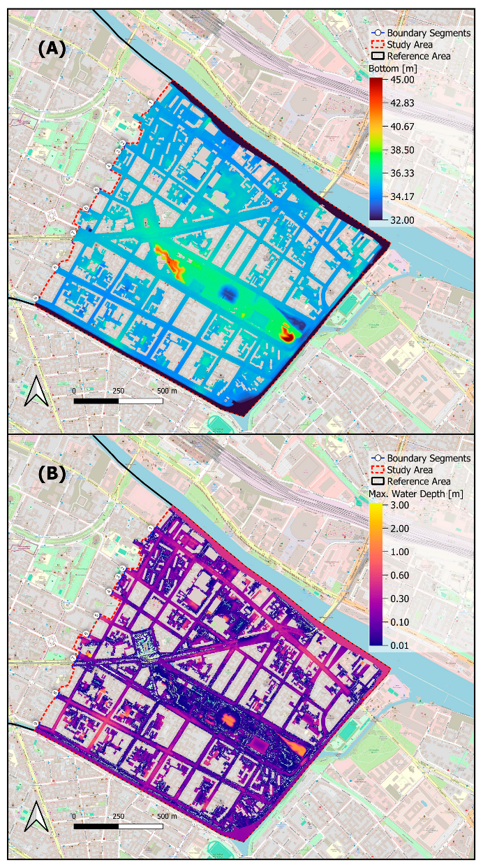
2.1. Study Domain, Reference Domain, and Precipitation Scenarios

The study domain is located in the Kreuzberg district of Berlin, Germany, covering approximately 2 km2. Figure 1 shows a map illustrating the almost rectangular shape of the study domain (red dashed line) and its embedding within the reference domain. The river Spree borders the top right of the study domain, the Landwehr Canal borders the bottom left, and both are connected at the bottom right via a sluice gate (marked with a blue star). These rivers serve as outlet BCs with a constant water level. The open boundary on the top left (red dashed line in the center of the map) cuts through the urbanized area and is divided into nine segments separated by buildings. Elevations within the study domain range from 32 to 45 m, but most of the domain’s elevation is within 33 to 36 m, and only a hill in Görlitzer Park has a higher elevation (Figure 2A).
The reference model is used to validate the BCs. It extends beyond the study domain’s open boundary (black solid line) but does not cross the bounding water bodies of the test model. The reference model covers an area of about 4 km2, twice the area of the study domain. Both the reference and the study models have open boundaries positioned perpendicular to streets.
Approximately one-third of both the study and reference areas are covered by buildings, represented as holes in the model, which affect effective rainfall. Water from building roof areas is added to the effective rainfall in the model for high-intensity precipitation events, assuming the storm drainage system is completely surcharged [46]. To ensure consistency, the same effective rainfall is used for both the test and reference models, despite slight differences in building coverage.
Three different one-hour block rainfall scenarios are investigated. The first scenario simulates an extreme precipitation event (HN999) with 100 mm of accumulated rainfall, yielding an effective rainfall of 150 mm over one hour, considering the effect of roof areas. This effective rainfall is added uniformly to every node in both models. The second scenario, based on the KOSTRA dataset for Germany, simulates a 100-year return period event (HN100) with 48.9 mm of accumulated rainfall [47] and an effective rainfall of 73.3 mm. The third scenario simulates a 30-year return period event (HN30) with 38.3 mm of accumulated rainfall [47]. Here, the effective rainfall is not adjusted, assuming the storm drainage system can handle the roof runoff. All scenarios include an additional two-hour simulation period post-rainfall to capture the flood dynamics. After three hours of total simulation time, the flow in the model subsides, and most of the water is at a standstill.

2.2. Modeling Software and Parameters

For conducting numerical simulations, this study utilizes the open-source TELEMAC system. Its hydrodynamic module, TELEMAC-2D, solves the full 2D Shallow Water Equations using either a finite-element scheme [48] or a finite-volume scheme. In this study, the finite-element scheme is applied with a semi-implicit solver on a triangulated mesh [49].
Although TELEMAC-2D includes several rainfall–runoff models, none are selected in this study. The objective is to isolate the influence of the open boundary as much as possible, necessitating the minimization of other factors such as heterogeneous land use, which would significantly affect rainfall–runoff modeling. Consequently, all infiltration processes are left out of consideration, and rain is directly added to the model using the rain-on-grid method in TELEMAC-2D [50].
The test model mesh consists of approximately 353,000 nodes and 669,000 elements, while the reference model mesh comprises about 768,000 nodes and 1,458,000 elements. The mean edge length in both meshes is 2.1 m. Node elevations are interpolated from a digital elevation model with a 1 × 1 m resolution (Figure 2A).
The Strickler roughness coefficients k s t are derived from land use data following guidelines from the LUBW [46]. Additionally, the LUBW recommendation for a depth-dependent roughness model is implemented in TELEMAC-2D. The Strickler roughness coefficients k s t are equivalent to 1 / m , with m the Manning roughness coefficient.
All input data are available from Berlin’s geoportal [51].

2.3. Boundary Conditions

Well-formulated BCs ensure a stable and accurate simulation representing the inflow and outflow at the model’s border, whereas inappropriate BCs can lead to inaccuracies in the solution, and possibly even numerical instabilities. Therefore, BCs must be defined with utmost care [48].
The test model domain in Berlin is confined by water bodies on three of the four sides (see Figure 1). These water bodies serve as BCs with fixed water levels, as they do not exhibit backwater impounding effects during pluvial floods in the study domain. Additionally, these water bodies also represent the initial state of the model.
The open boundary on the left side of the study domain is divided by buildings into nine boundary segments (see blue lines Figure 1, numbered 1 through 9). The buildings are modeled as rigid boundaries. Three of the nine boundary segments (1, 8, and 9) have negative slopes at the boundary, indicating topographical model inlets. The remaining boundary segments (2, 3, 4, 5, 6, and 7) have a positive slope at the boundary, suggesting possible outlets for the study domain. Segments 3 and 7 are particularly challenging due to their heterogeneous cross-sections: segment 3 is within an inner courtyard, and segment 7 spans multiple street crossings, complicating the formulation of BCs for these segments.
In total, five different BCs are tested on all segments and then segmentally combined in an optimized setup. The different BCs are explained in detail in the following subsections.

2.3.1. Closed Wall

A closed wall (CW) is a rigid BC, preventing any water flow through the boundary. Water will impound at the boundary and cannot leave the model domain. This is implemented either by setting all velocities at the wall to zero or by setting the velocity perpendicular to the wall to zero and implementing tangential stress at the wall using wall friction [48].

2.3.2. Zero Water Depth

The zero water depth (ZWD) BC maintains a fixed water depth of zero at the boundary. This creates a suction effect that increases the velocity near the boundary, allowing water to leave the domain.

2.3.3. Stage–Discharge Curve

A stage–discharge curve (SDC) is a well-established BC in fluvial hydraulics. It calculates the water depth at the boundary based on the current discharge using a predefined SDC. For this study, the SDCs are derived assuming normal flow conditions through the boundaries:
Q = b · k s t · h 5 3 · I s
Here, Q is the discharge through the boundary, b is the width of the boundary, k s t is the Strickler roughness coefficient, h is the water depth, and I S the slope normal to the boundary. I S is calculated using the average elevations of cross-sections 20 m outside and inside the model domain. Since boundary segments 1, 8, and 9 have negative slopes, SDCs cannot be calculated for these segments, and a CW BC is assumed for them.

2.3.4. Drainage Reservoir

The drainage reservoir (DR) BC creates small pools at each open boundary segment, acting as drainage reservoirs. The mesh is extended by 100 m perpendicular to each open boundary segment. The elevation of the extended mesh parts is set so that the minimum elevation at the original open boundary segment is one meter higher than at the new open boundary segment. A parabolic descent is implemented within the 100 m extension, and the new open boundary segment is set to a constant water depth of 0.25 m. This configuration allows water to flow slowly over the parabolic profile into the DR, ensuring a stable boundary condition. The mesh extension for the DR BC adds approximately 10,000 nodes and 20,000 elements.

2.3.5. Drainage Element
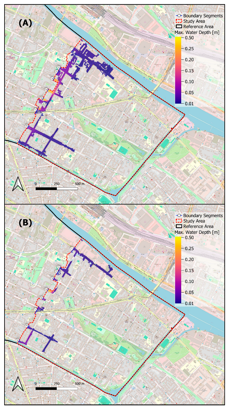
The drainage element (DE) BC is similar to the DR BC but does not extend the mesh. Instead, it lowers the elevation of nodes directly at the open boundary segment by 0.5 m below the minimum node elevation at the open boundary segment. A constant water depth of 0.25 m is then defined at the open boundary segment, resulting in minor inundation of the elements directly at the boundary.

2.4. Validation

For validation, two simulations are additionally conducted with the reference model for each scenario (HN999, HN100, HN30). Given that the reference model also includes several open boundary segments, it is crucial to assess the influence of these open boundary segments. One reference simulation is conducted with CW BCs and one with ZWD BCs. Figure 3 illustrates, for the HN999 event, the absolute difference in simulated maximum water depth between the CW and ZWD BCs in the reference model. Differences smaller than 1 mm are neglected.
Figure 3 confirms that the influence of the two different BCs in the reference model does not propagate into the domain of the test model (outlined by the red dashed line). Differences exceeding 1 mm are observed only at isolated nodes. Given the marginal number of these instances relative to the overall number of nodes, the reference model is deemed suitable for validating the different open boundary conditions of the test model. The influence of the CW and the ZWD BCs further decreases for the HN100 and HN30 events compared to the H999 event.

2.5. Statistical Measures

The following goodness-of-fit criteria quantitatively assess the different open BCs for the whole study domain (1 through 4) or per segment (5).
  • Vol_dif [m3]: The difference in total maximum volume between the test model under different open BCs and the reference model within the study domain.
  • PBIAS and PBIAS_sub [%]: The percent bias (PBIAS) investigates the difference in maximum water depth at all nodes between the reference model and the test models. Negative PBIAS values indicate that the test model underpredicts the maximum water depths compared to the reference model, while positive PBIAS values indicate overestimation. The PBIAS is sensitive to the model’s area. Larger model areas tend to dilute the influence of BCs, resulting in smaller PBIAS values, since the region of influence of the BCs is decreasing in comparison to the overall model’s area. To address this, PBIAS_sub is calculated within a subset of the model domain. This subset includes nodes where the maximum water depth deviation from the reference model exceeds 1 cm in at least one of the BCs.
  • MAE and MAE_sub [mm]: The mean absolute error (MAE) is a unit-based statistical measure that quantifies the average deviation in maximum water depth at every node between the test models and the reference model. It provides an overall measure of model accuracy. Same as PBIAS, the MAE is sensitive to the model’s area, and MAE_sub is calculated accordingly.
  • DBI [m]: A region of influence from the BCs is defined by the area where the absolute difference in maximum simulated water depth between the test and reference models exceeds specific thresholds (1 mm and 1 cm). This area is normalized by the cumulative length of the open boundary segments. This normalized measure is also not sensitive to the model’s area and is termed “distance of boundary influence” (DBI).
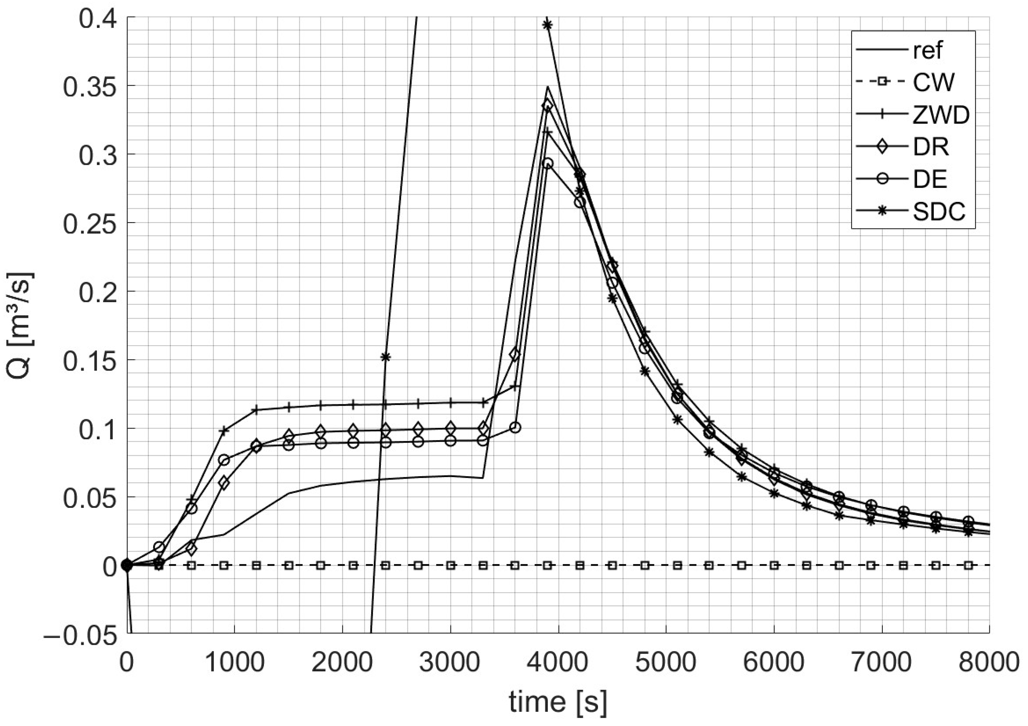
  • NSE: The Nash–Sutcliffe efficiency (NSE) is used to assess the discharge across each boundary segment, with the segmental discharges from the reference model serving as the observed values. This assessment provides a deeper insight into the behavior of BCs at individual boundary segments.
Due to the low gradients in the model, flow velocities in the test model are minimal and, therefore, not statistically investigated.

3. Results

3.1. Effects of the Precipitation Intensity on the BCs

First, the effects of precipitation intensity on BCs were assessed across three rainfall scenarios. Figure 4A,B, comparing the absolute difference in maximum water depth between the reference model and the test model applying CW BCs, highlight how the precipitation intensity of the HN999 event and the HN30 impacts BC performance. The maximum water depth of the HN999 event for the test model is illustrated in Figure 2B for further perspective.
For the HN999 event, BCs exert a greater influence due to increased water volume in the model, affecting larger areas. This greater influence is reflected in the statistical measures across all BCs tested. Specifically, the MAE is 3.7 mm for the HN999 event (see also CW in Table 1) and only 0.9 mm for HN30. The difference in total maximum volume between the reference model and the test model is 2133 m3 for the HN999 event and only 65 m3 for the HN30. Finally, the DBI with a 1 mm threshold depth is 468 m for the HN999 event and 162 m for the HN30. As the BCs’ impact is considerably larger for higher-precipitation events, the detailed investigation of the discharges across boundary segments will focus exclusively on the HN999 event from now on.

3.2. Evaluation of Difference in Volume, Area and Maximum Water Depth

Table 1 lists the statistical measures for the different BCs used on the HN999 event. The DBI 1 mm shows that the CW performs worse by over 30 m compared to the other BCs in this metric, while the DBI 1 mm values of the other BCs lie close to each other. The DBI 1 cm is larger for the CW, DE, and ZWD BCs than for the SDC BCs by around 60 to 70 m, whereas the DBI 1 cm of the DR BCs is only around 40 m larger. The Vol_dif shows an overprediction by the CW BCs, whereas all other BCs underpredict compared to the reference model. SDC BCs show the best results using this metric. The PBIAS values further support these trends.
The MAE shows that, in total, the BCs introduce an average error of up to 3.7 mm in maximum water depth prediction. The lowest MAE values are with the DR (2.0 mm) and SDC (1.9 mm). All these MAEs are small globally, as they are computed over the complete model domain, including the areas in which the BCs do not influence the results.
The PBIAS_sub and MAE_sub are calculated for a relevant subset covering approximately 10% of the test model area near the open boundary. The highest MAE_sub is 39.4 mm for the CW BCs. The lowest MAE_sub is again obtained for the DR (19.8 mm) and the SDC (18.8 mm).

3.3. Discharges across Open Boundaries

Three different types of open boundary segments were analyzed in this study: topographical inlets (Figure 5), topographical outlets (Figure 6), and heterogeneous cross-sections (Figure 7). The hydrograph from the reference model is shown as a black line without markers in all figures. Inflow into the test model domain is indicated by negative discharge values and outflow by positive discharge values.

3.3.1. Topographical Inlets

At topographical inlet segment 9 (see Figure 1 for the location), the reference model exhibits a maximum discharge of −0.125 m3/s flowing into the test model domain (see Figure 1). The CW BC shows no flow across the boundary in any segment, just like the SDC BC at segment 9, implemented as CW BCs at topographical inlets. Conversely, other BCs permit outflow from the test model: the DE BC peaks at 0.848 m3/s, the ZWD at 0.423 m3/s, and the DR BC at 0.212 m3/s. The NSE ranges poorly from −0.61 (CW/SDC) to −147 (DE) for this segment, with similar behaviors observed in the other topographical inlet segments 1 and 8 (see the corresponding columns in Table 2).

3.3.2. Topographical Outlets

Figure 6 illustrates the hydrographs for different BCs compared to the reference model at the topographical outlet segment 5. The reference model has a peak discharge of 0.850 m3/s with 2869 m3 leaving the test model domain during the event. The SDC BC and the DR BC slightly overpredict the reference hydrograph with peak discharges of 0.885 m3/s and 0.876 m3/s and volumes of 2912 m3 and 2887 m3, respectively. The DE and ZWD BCs underestimate the reference hydrograph, peaking at 0.715 m3/s and 0.631 m3/s, with volumes of 2108 m3 and 2076 m3 leaving the test model. The NSEs are excellent for the SDC (0.998) and DR BCs (0.998), and lower for the DE (0.91) and ZWD BCs (0.88). Generally, SDC BC performs best across all topographical outlet segments (lowest NSE 0.86, see Table 2, columns for topographical outlet segments 2, 4, 5, and 6), with the DR BC also yielding satisfactory NSEs (lowest NSE 0.38), whereas the ZWD and DE BCs show good NSEs only for specific segments.

3.3.3. Heterogeneous Cross-Sections

Figure 7 shows the hydrographs at boundary segment 7, a heterogeneous cross-section where three different streets intersect within the test model domain. The boundary segment is then located a bit away from the crossing, yet still cuts through two streets. The reference model peaks at 0.349 m3/s with 745 m3 leaving the domain. The SDC BC presents an unstable behavior, initially releasing water into the test model with a negative discharge of up to −0.345 m3/s and subsequently overestimating the peak discharge at 0.560 m3/s (both values lying beyond the borders of Figure 7). This is attributed to the instability of the SDC BC for small water depths along inhomogeneous cross-sections. The other BCs present more stable solutions, though they are all overestimating the initial discharge. The DR BC peaks at 0.335 m3/s with 822 m3 leaving the domain, the ZWD BC at 0.316 m3/s with 912 m3, and the DE BC at 0.292 m3/s with 804 m3, showing the closest volume balance to the model.
The NSE values for segment 7 are highest for the DR BC (0.93) and satisfactory for the DE BC (0.87) and the ZWD BC (0.81). The CW BC (−0.71) and especially the SDC BC (−5.26) indicate poor results (see Table 2).
The other boundary segment with a heterogeneous cross-section (the inner courtyard at segment 3) does not yield suitable NSEs by any BC. Yet, with a maximum reference discharge of only 0.052 m3/s and a total volume of only 0.9 m3 crossing the boundary, its impact on the global results is several orders of magnitude lower than that of the other segments.

3.4. Optimized Segmental Combination of BCs

Following the analysis of the results for each tested NC, an optimized BC setup was devised:
  • Topographical inlets: The CW BC was selected since it had brought about the best approximation of the reference model amongst the analyzed BCs (see Figure 5 and Table 2).
  • Topographical outlets: The SDC and DR BC both performed well, yet the SDC BC was preferred, mainly in view of the SDC BC’s more consistent performance when considering the NSE values at segments 2 and 6 (see Table 2).
  • Heterogeneous type cross-section, segment 7: The SDC and CW BCs performed poorly for segment 7, whilst a remarkably accurate estimation, also reflected by the NSE value, was obtained with the DR BC (Figure 7, Table 2), and therefore, the DR BC was selected.
  • Heterogeneous-type cross-section, segment 3: Neither of the BCs performed well here; the CW BC was chosen because it yielded the best NSE value (Table 2).
Starting with this described set of BCs, the HN999 event was simulated again, and its results were analyzed. The NSE values at each boundary segment for this optimized setup and its statistical evaluation of global metrics are shown in the top lines of Table 3 and Table 4, respectively. The other lines reproduce Table 1 and Table 2 for comparison purposes.
Regarding the NSE values in Table 3 first, the following become apparent:
  • For the topographical inlet segments 1, 8, and 9, for which the CW BC was adopted, the optimized segmental combination of BCs has identical NSE values to the ones in a CW-BC-only setup. This is according to expectations due to the physical meaning of the CW BC. The same holds for the heterogeneous cross-section segment 3.
  • For the topographical outlet segments 2, 4, 5, and 6, the NSEs appear largely unaffected when comparing the optimized segmental combination with the SDC-BC-only setup. However, for segment 2, an improvement in the NSE from 0.86 to 0.92 is noted.
  • For the heterogeneous cross-section segment 7, the DR BC NSE of 0.93 was not fully maintained. Yet, the obtained NSE of 0.87 with the optimized segmental combination of BCs is still solid compared to the NSEs originally obtained for any other BC simulation.
Similar signs of robustness are recognized when evaluating the global statistical metrics in Table 4 regarding volumes, area of influence, and maximum water depths. The optimized segmental combination of BCs outperforms each individual BC regarding DBI 1 mm, DBI 1 cm, MAE, and MAE_sub. The same holds for Vol_dif, PBIAS, and PBIAS_sub, except for the SDC BCs, which seem to yield better results at first sight.
However, analyzing this more closely, it appears that these better results are, in fact, due to the SDC BCs’ instability at segments 3 and 7, which has introduced water into the model and thereby added extra volume to the simulation. This additional volume, whilst enhancing the computed statistical performance for Vol_dif, PBIAS, and PBIAS_sub, is, in fact, non-physical and occurs at the boundaries where the SDC BC performs poorly, as evidenced in Figure 7.
In summary, the optimized segmental combination of BCs appears to strike a solid balance between maintaining physical accuracy across different types of boundary segments while minimizing computational resources, hence providing a robust framework for accurate flood modeling in an urban environment in topographically varying domains.

4. Discussion

4.1. Performance and Selection of BCs

The results of this study underscore the critical importance of carefully selecting appropriate segmental BCs for urban hydrodynamic flood models based on the topography. Specifically, topographical outlets can be accurately modeled using SDC BCs or DR BCs, with SDC BCs slightly outperforming DR BCs.
Potential inflow at topographical inlets cannot be modeled without coupling the hydraulic model to another model or incorporating extra hydrological information at the boundary segments. One potential solution could consist of constructing simple inflow hydrographs based on precipitation data and hydrological response units, adapting the unit hydrograph theorem [52] for small domains. Although such lumped approaches can approximate inflow qualitatively, it remains improbable that high precision can be achieved, since urban domains have a high hydraulic complexity.
Heterogeneous cross-sections require special attention. The source of heterogeneity is specific to each case, making it difficult to provide a universally optimal solution proposal. For example, boundary segment 3 in this study has only minimal discharge values and has, therefore, a lower impact on overall model results compared to other boundary segments.
In contrast, boundary segment 7 significantly impacts the overall model results due to higher discharge values. This segment is located shortly after the intersection of three different streets, complicating the formulation of an appropriate BC. A potential solution is to divide the boundary segment into smaller, more homogeneous segments, treating some as outflows and others as CWs based on topography. The SDC BCs did not perform well for heterogeneous cross-sections, due to the varying topography along the cross-section, which impedes the definition of SDCs.

4.2. Preprocessing Requirements

The investigated BCs also differ in their preprocessing requirements. CW BCs and ZWD BCs are amongst the more accessible ones, requiring no changes in the mesh, topography, or additional knowledge about the model.
The SDC BCs, however, require formulating a stage–discharge relationship using Manning’s formula, introducing uncertainty due to roughness value and slope definition. Defining the slope in urban domains, where it can vary greatly along a street, adds to this complexity.
DE BCs require additional preprocessing to lower the elevation of nodes near the boundary and to fill drainage elements with water before the simulation, either by defining a water level or running a precursor simulation.
The DR BCs demand higher preprocessing overhead, requiring mesh extension at boundary segments and defining a descending ramp profile along the mesh extension. In exchange for this overhead, DR BCs provided stable results and performed well statistically. The additional computational time due to the increased number of elements was negligible since the number of added elements was smaller than 3%.

4.3. Mutual Interference of BCs

The mutual interference of different boundary segments’ BCs must also be taken into consideration. The optimized setup shows that BCs of different segments influence each other. This is evidenced by variations in NSEs for some segments compared to simulations with the same BCs applied to all segments. For example, the NSE in segment 2 is better in the optimized setup than in the SDC BC for all segments, while the DR BC in segment 7 performs slightly worse in the optimized setup (see Table 3).
This interference is not surprising due to connected inundation areas between boundary segments, yet remains of lesser importance for this model domain. However, for other domains, this interference might become more dominant.

4.4. Pre-Assessment of Sensitivity of the BC Selection

BCs must always be defined when setting up a hydrodynamic flood model. While this study emphasizes the importance of carefully selecting segmental boundary conditions, it acknowledges that a comprehensive assessment of each individual boundary segment can be time-consuming.
Therefore, this study recommends performing a sensitivity analysis to pre-assess the impact of the boundary on overall model results prior to formulating segmental boundary conditions. This can be achieved by running the model twice with different BCs, such as CW BCs and ZWD BCs, as carried out for the reference model in this study. These BCs are straightforward to implement and fundamentally different in their methods. If the differences in solutions are negligible, the model results are deemed not sensitive to the treatment of the boundary segments. In this case, the simpler approach of using a CW BC on all segments is justified and the process of determining the optimized BC for each individual boundary segment can be omitted.

4.5. Limitations of the Study

This study utilizes the hydrodynamic module TELEMAC-2D of the open-source TELEMAC system, which solves the full 2D Shallow Water Equations. The BCs tested and described in this study are transferable to various hydrodynamic solvers and can be applied across numerous widely used flood modeling software packages, such as LISFLOOD-FP [53], HEC-RAS [54], or MIKE FLOOD [55]. Typically, the results of the specific BCs may slightly vary depending on the software used.
As already described in Section 2.1 and Section 2.2, this study has assumed that the storm drainage system is either completely surcharged or fully able to handle the runoff from roof areas. Hence, it does not include rainfall–runoff or urban storm drainage modeling at this stage. With a view to coupling 1D storm drainage models with 2D surface models, additional boundary conditions for the 2D model would be introduced, as water could possibly transfer between the storm drainage system and the surface. This interaction would directly affect the volume of water in the model domain, thereby impacting the boundary conditions. However, the additional BCs from such coupling are considered internal BCs; therefore, BCs at open boundaries of the 2D model would still need to be addressed. In order to do so, it is expected that the findings of this study remain applicable to 1D-2D coupled models.
The present study relies on a validation method that utilizes a larger-extent reference model. Even though this validation method was found robust, a higher degree of confidence in the results could be achieved by validating the BCs with inundation data from actual pluvial flood events. Given the general scarcity of such data, the adopted validation approach offers a solid alternative for defining the BCs.

5. Conclusions

In this study, an optimization approach characterized by a combination of segment-tailored boundary conditions (BCs) for simulating pluvial urban floods in varying topography has been proposed. First, each type of BC was analyzed individually and then the different BCs were combined segment-wise to obtain an improved setup. This combined BC setup outperformed all other models using one and the same BC for all segments.
The findings show that careful selection of appropriate segmental BCs is of critical importance to ensure high accuracy. For topographical inlets, closed wall BCs are recommended, while stage–discharge curves are advisable for topographical outlets. For more heterogeneous cross-sections, no universal recommendation can be given; however, a drainage reservoir BC provides a stable approach. As a general guideline, conducting an initial sensitivity analysis of the model boundaries applying two different BCs can help determine whether the BCs in the flood model require detailed attention or if they have a minimal impact on the results.
Future research could include a detailed sensitivity analysis of different BCs. This is particularly interesting regarding the definition of slope for stage–discharge curves and the impact of the length and slope of the descending ramp for drainage reservoirs.

Author Contributions

Conceptualization, L.F.D.V., N.R. and K.B.; investigation, L.F.D.V.; methodology, L.F.D.V., N.R., K.M., A.D. and K.B.; project administration, L.F.D.V. and N.R.; software, L.F.D.V. and K.M.; supervision, N.R. and K.B.; validation, L.F.D.V.; visualization, L.F.D.V. and K.M.; writing—original draft, L.F.D.V.; writing—review and editing, L.F.D.V., N.R., K.M., A.D. and K.B. All authors have read and agreed to the published version of the manuscript.

Funding

This work was supported by the German Federal Ministry of Education and Research within the federal program “Water: N—Research and Innovation for Sustainability” as part of the project “Inno_MAUS” under grant number 02WEE1632B.

Data Availability Statement

Simulation data can be retrieved here: “https://osf.io/ycj3u/?view_only=36fdcafa0fd14dfaa6103c4041bceaec” (accessed on 2 July 2024). For further information, please contact the corresponding author [L.F.D.V.].

Conflicts of Interest

The authors declare no conflicts of interest.

References

  1. IPCC. Water: Climate Change 2022: Impacts, Adaptation and Vulnerability; IPCC: Geneva, Switzerland, 2022. [Google Scholar]
  2. IPCC. Weather and Climate Extreme Events in a Changing Climate: Climate Change 2021: The Physical Science Basis; IPCC: Geneva, Switzerland, 2021. [Google Scholar]
  3. Myhre, G.; Alterskjær, K.; Stjern, C.W.; Hodnebrog, Ø.; Marelle, L.; Samset, B.H.; Sillmann, J.; Schaller, N.; Fischer, E.; Schulz, M.; et al. Frequency of extreme precipitation increases extensively with event rareness under global warming. Sci. Rep. 2019, 9, 16063. [Google Scholar] [CrossRef] [PubMed]
  4. Uhe, P.; Mitchell, D.; Bates, P.D.; Allen, M.R.; Betts, R.A.; Huntingford, C.; King, A.D.; Sanderson, B.M.; Shiogama, H. Method Uncertainty Is Essential for Reliable Confidence Statements of Precipitation Projections. J. Clim. 2021, 34, 1227–1240. [Google Scholar] [CrossRef]
  5. Prokić, M.; Savić, S.; Pavić, D. Pluvial flooding in urban areas across the European continent. Geogr. Pannonica 2019, 23, 216–232. [Google Scholar] [CrossRef]
  6. Nicklin, H.; Leicher, A.M.; Dieperink, C.; Leeuwen, K. Understanding the Costs of Inaction—An Assessment of Pluvial Flood Damages in Two European Cities. Water 2019, 11, 801. [Google Scholar] [CrossRef]
  7. Bulti, D.T.; Abebe, B.G. A review of flood modeling methods for urban pluvial flood application. Model. Earth Syst. Environ. 2020, 6, 1293–1302. [Google Scholar] [CrossRef]
  8. Teng, J.; Jakeman, A.J.; Vaze, J.; Croke, B.; Dutta, D.; Kim, S. Flood inundation modelling: A review of methods, recent advances and uncertainty analysis. Environ. Model. Softw. 2017, 90, 201–216. [Google Scholar] [CrossRef]
  9. HSB. Ermittlung von Überflutungsgefahren mit Vereinfachten und Detaillierten Hydrodynamischen Modellen. Praxisleitfaden, Erstellt im Rahmen des DBU-Forschungsprojekts “KLASII”; HSB: Bremen, Germany, 2017. [Google Scholar]
  10. Guo, K.; Guan, M.; Yu, D. Urban surface water flood modelling—A comprehensive review of current models and future challenges. Hydrol. Earth Syst. Sci. 2020, 25, 2843–2860. [Google Scholar] [CrossRef]
  11. Bates, P.D. Flood Inundation Prediction. Annu. Rev. Fluid Mech. 2022, 54, 287–315. [Google Scholar] [CrossRef]
  12. van Dijk, E.; van der Meulen, J.; Kluck, J.; Straatman, J.H.M. Comparing modelling techniques for analysing urban pluvial flooding. Water Sci. Technol. 2014, 69, 305–311. [Google Scholar] [CrossRef]
  13. Yang, Y.; Sun, L.; Li, R.; Yin, J.; Yu, D. Linking a Storm Water Management Model to a Novel Two-Dimensional Model for Urban Pluvial Flood Modeling. Int. J. Disaster Risk Sci. 2020, 11, 508–518. [Google Scholar] [CrossRef]
  14. Leandro, J.; Chen, A.S.; Djordjević, S.; Savić, D.A. Comparison of 1D/1D and 1D/2D Coupled (Sewer/Surface) Hydraulic Models for Urban Flood Simulation. J. Hydraul. Eng. 2009, 135, 495–504. [Google Scholar] [CrossRef]
  15. Reinstaller, S.; Krebs, G.; Pichler, M.; Muschalla, D. Identification of High-Impact Uncertainty Sources for Urban Flood Models in Hillside Peri-Urban Catchments. Water 2022, 14, 1973. [Google Scholar] [CrossRef]
  16. Fan, Y.; Ao, T.; Yu, H.; Huang, G.; Li, X. A Coupled 1D-2D Hydrodynamic Model for Urban Flood Inundation. Adv. Meteorol. 2017, 2017, 2819308. [Google Scholar] [CrossRef]
  17. Russo, B.; Sunyer, D.; Velasco, M.; Djordjević, S. Analysis of extreme flooding events through a calibrated 1D/2D coupled model: The case of Barcelona (Spain). J. Hydroinformatics 2015, 17, 473–491. [Google Scholar] [CrossRef]
  18. Luo, P.; Luo, M.; Li, F.; Qi, X.; Huo, A.; Wang, Z.; He, B.; Takara, K.; Nover, D.; Wang, Y. Urban flood numerical simulation: Research, methods and future perspectives. Environ. Model. Softw. 2022, 156, 105478. [Google Scholar] [CrossRef]
  19. Popescu, I. Computational Hydraulics: Numerical Methods and Modelling; IWA Publishing: London, UK, 2014; ISBN 9781780400457. [Google Scholar]
  20. Deletic, A.; Dotto, C.; McCarthy, D.T.; Kleidorfer, M.; Freni, G.; Mannina, G.; Uhl, M.; Henrichs, M.; Fletcher, T.D.; Rauch, W.; et al. Assessing uncertainties in urban drainage models. Phys. Chem. Earth Parts A/B/C 2012, 42–44, 3–10. [Google Scholar] [CrossRef]
  21. Bates, P.D.; Pappenberger, F.; Romanowicz, R.J. Uncertainty in Flood Inundation Modelling. In Applied Uncertainty Analysis for Flood Risk Management; Beven, K., Hall, J., Eds.; Imperial College Press: London, UK, 2014; pp. 232–269. ISBN 978-1-84816-271-6. [Google Scholar]
  22. Bermúdez, M.; Neal, J.C.; Bates, P.D.; Coxon, G.; Freer, J.E.; Cea, L.; Puertas, J. Quantifying local rainfall dynamics and uncertain boundary conditions into a nested regional-local flood modeling system. Water Resour. Res. 2017, 53, 2770–2785. [Google Scholar] [CrossRef]
  23. Pappenberger, F.; Matgen, P.; Beven, K.J.; Henry, J.-B.; Pfister, L.; Fraipont, P. Influence of uncertain boundary conditions and model structure on flood inundation predictions. Adv. Water Resour. 2006, 29, 1430–1449. [Google Scholar] [CrossRef]
  24. Mason, D.C.; Schumann, G.; Bates, P.D. Data Utilization in Flood Inundation Modelling. In Flood Risk Science and Management; Pender, G., Faulkner, H., Eds.; Wiley: Hoboken, NJ, USA, 2010; pp. 209–233. ISBN 9781405186575. [Google Scholar]
  25. Rohmat, F.I.W.; Sa’adi, Z.; Stamataki, I.; Kuntoro, A.A.; Farid, M.; Suwarman, R. Flood modeling and baseline study in urban and high population environment: A case study of Majalaya, Indonesia. Urban Clim. 2022, 46, 101332. [Google Scholar] [CrossRef]
  26. Echeverribar, I.; Morales-Hernández, M.; Brufau, P.; García-Navarro, P. 2D numerical simulation of unsteady flows for large scale floods prediction in real time. Adv. Water Resour. 2019, 134, 103444. [Google Scholar] [CrossRef]
  27. Bates, P. Fundamental limits to flood inundation modelling. Nat. Water 2023, 1, 566–567. [Google Scholar] [CrossRef]
  28. Jafarzadegan, K.; Alipour, A.; Gavahi, K.; Moftakhari, H.; Moradkhani, H. Toward improved river boundary conditioning for simulation of extreme floods. Adv. Water Resour. 2021, 158, 104059. [Google Scholar] [CrossRef]
  29. Haile, A.; Rientjes, T. Uncertainty issues in hydrodynamic flood modeling. In Proceedings of the 5th International Symposium on Spatial Data Quality SDQ 2007, Modelling Qualities in Space and Time, ITC, Enschede, The Netherlands, 13–15 June 2007. [Google Scholar]
  30. Cea, L.; Garrido, M.; Puertas, J. Experimental validation of two-dimensional depth-averaged models for forecasting rainfall–runoff from precipitation data in urban areas. J. Hydrol. 2010, 382, 88–102. [Google Scholar] [CrossRef]
  31. David, A.; Schmalz, B. A Systematic Analysis of the Interaction between Rain-on-Grid-Simulations and Spatial Resolution in 2D Hydrodynamic Modeling. Water 2021, 13, 2346. [Google Scholar] [CrossRef]
  32. Hofmann, J.; Schüttrumpf, H. Risk-Based and Hydrodynamic Pluvial Flood Forecasts in Real Time. Water 2020, 12, 1895. [Google Scholar] [CrossRef]
  33. Kim, H.; Keum, H.; Han, K. Real-Time Urban Inundation Prediction Combining Hydraulic and Probabilistic Methods. Water 2019, 11, 293. [Google Scholar] [CrossRef]
  34. Nguyen, P.; Thorstensen, A.; Sorooshian, S.; Hsu, K.; AghaKouchak, A.; Sanders, B.; Koren, V.; Cui, Z.; Smith, M. A high resolution coupled hydrologic–hydraulic model (HiResFlood-UCI) for flash flood modeling. J. Hydrol. 2016, 541, 401–420. [Google Scholar] [CrossRef]
  35. Son, A.-L.; Kim, B.; Han, K.-Y. A Simple and Robust Method for Simultaneous Consideration of Overland and Underground Space in Urban Flood Modeling. Water 2016, 8, 494. [Google Scholar] [CrossRef]
  36. Hénonin, J.; Hongtao, M.; Zheng-Yu, Y.; Hartnack, J.; Havnø, K.; Gourbesville, P.; Mark, O. Citywide multi-grid urban flood modelling: The July 2012 flood in Beijing. Urban Water J. 2015, 12, 52–66. [Google Scholar] [CrossRef]
  37. Hunter, N.M.; Bates, P.D.; Neelz, S.; Pender, G.; Villanueva, I.; Wright, N.G.; Liang, D.; Falconer, R.A.; Lin, B.; Waller, S.; et al. Benchmarking 2D hydraulic models for urban flooding. Proc. Inst. Civ. Eng.-Water Manag. 2008, 161, 13–30. [Google Scholar] [CrossRef]
  38. Hartnett, M.; Nash, S. High-resolution flood modeling of urban areas using MSN_Flood. Water Sci. Eng. 2017, 10, 175–183. [Google Scholar] [CrossRef]
  39. Saad, H.A.; Habib, E.H.; Miller, R.L. Effect of Model Setup Complexity on Flood Modeling in Low-Gradient Basins. J. Am. Water Resour. Assoc. 2021, 57, 296–314. [Google Scholar] [CrossRef]
  40. Bruwier, M.; Mustafa, A.; Aliaga, D.G.; Archambeau, P.; Erpicum, S.; Nishida, G.; Zhang, X.; Pirotton, M.; Teller, J.; Dewals, B. Influence of urban pattern on inundation flow in floodplains of lowland rivers. Sci. Total Environ. 2018, 622–623, 446–458. [Google Scholar] [CrossRef] [PubMed]
  41. de Almeida, G.; Bates, P.; Ozdemir, H. Modelling urban floods at submetre resolution: Challenges or opportunities for flood risk management? J. Flood Risk Manag. 2018, 11, S855–S865. [Google Scholar] [CrossRef]
  42. Zhao, G.; Balstrøm, T.; Mark, O.; Jensen, M.B. Multi-Scale Target-Specified Sub-Model Approach for Fast Large-Scale High-Resolution 2D Urban Flood Modelling. Water 2021, 13, 259. [Google Scholar] [CrossRef]
  43. Paquier, A.; Bazin, P.H.; El Kadi Abderrezzak, K. Sensitivity of 2D hydrodynamic modelling of urban floods to the forcing inputs: Lessons from two field cases. Urban Water J. 2020, 17, 457–466. [Google Scholar] [CrossRef]
  44. Bermúdez, M.; Cea, L.; Puertas, J. A rapid flood inundation model for hazard mapping based on least squares support vector machine regression. J. Flood Risk Manag. 2019, 12, e12522. [Google Scholar] [CrossRef]
  45. OpenStreetMap Contributors. OpenStreetMap. Available online: https://www.openstreetmap.org/ (accessed on 2 July 2024).
  46. LUBW. Anhänge 1 a, b, c zum Leitfaden Kommunales Starkregenrisikomanagement in Baden-Württemberg; LUBW: Karlsruhe, Germany, 2020. [Google Scholar]
  47. Junghänel, T.; Bär, F.; Deutschländer, T.; Haberlandt, U.; Otte, I.; Shehu, B.; Stockel, H.; Stricker, K.; Thiele, L.-B.; Willems, W. Methodische Untersuchungen zur Novellierung der Starkregenstatistik für Deutschland (MUNSTAR). Synthesebericht; DWD: Offenbach, Germany, 2022. [Google Scholar]
  48. Hervouet, J.-M. Hydrodynamics of Free Surface Flows; Wiley: Hoboken, NJ, USA, 2007; ISBN 9780470035580. [Google Scholar]
  49. EDF. TELEMAC-2D: User Manual. Version v8p4; EDF: Paris, France, 2022; 8p. [Google Scholar]
  50. Godara, N.; Bruland, O.; Alfredsen, K. Simulation of flash flood peaks in a small and steep catchment using rain-on-grid technique. J. Flood Risk Manag. 2023, 16, e12898. [Google Scholar] [CrossRef]
  51. Senatsverwaltung Berlin. Geoportal Berlin. Available online: https://www.berlin.de/sen/sbw/stadtdaten/geoportal/ (accessed on 2 July 2024).
  52. Sherman, L.K. The relation of hydrographs of runoff to size and character of drainage-basins. Trans. AGU 1932, 13, 332. [Google Scholar] [CrossRef]
  53. Bates, P.; Trigg, M.; Neal, J.; Dabrowa, A. LISFLOOD-FP: User Manual. Code Release 5.9.6; University of Bristol: Bristol, UK, 2013. [Google Scholar]
  54. Brunner, G. HEC-RAS: River Analysis System User’s Manual. Version 5.0; US Army Corps of Engineers: Washington, DC, USA, 2016. [Google Scholar]
  55. DHI Water and Environment. MIKE FLOOD.: DHI Software. User Manual; DHI Water and Environment: Hørsholm, Denmark, 2019. [Google Scholar]
Figure 1. The study domain (red dashed outline) embedded in the reference domain (additional black line) in Berlin. The open boundary is split into segments 1–9 (marked with blue lines). Background map from OpenStreetMap [45].
Water 16 02448 g001
Figure 2. (A): Interpolated elevation of the test model. (B): Maximum water depth of the test model for the HN999 event.
Water 16 02448 g002
Figure 3. Absolute difference in maximum water depth between the CW and ZWD BC in the reference model for the HN999 event. The red line shows the boundary of the test model that is embedded in the reference model. Background map from OpenStreetMap.
Water 16 02448 g003
Figure 4. (A,B): Comparison of the difference in absolute maximum water depth between the reference model and the test model when using a CW BC and a threshold of 1 mm. (A) is the difference for the HN999 event with 150 mm effective precipitation, and (B) is the difference for HN30 with 38.3 mm effective precipitation.
Water 16 02448 g004
Figure 5. Hydrographs at boundary segment 9, which is a topographical inlet. The solution from the reference model is compared with the solutions of the tested BCs for the HN999 event.
Water 16 02448 g005
Figure 6. Hydrographs at boundary segment 5, a topographical outlet. The solution from the reference model is compared with the solutions of the tested BCs for the HN999 event.
Water 16 02448 g006
Figure 7. Hydrographs at boundary segment 7, a heterogeneous cross-section. The solution from the reference model is compared with the solutions of the tested BCs for the HN999 event.
Water 16 02448 g007
Table 1. Statistical evaluation of global metrics using different BCs for the HN999 event.
BCDBI 1 mm
[m]
DBI 1 cm
[m]
Vol_dif
[m3]
PBIAS
[%]
PBIAS_sub
[%]
MAE
[mm]
MAE_sub
[mm]
CW46826621331.28.93.739.4
ZWD433259−3034−1.7−10.62.525.0
DR427239−2372−1.3−8.32.019.8
DE436265−3012−1.6−10.32.727.3
SDC422198−781−0.4−2.41.918.8
Table 2. The NSE values for all tested BCs at each boundary segment for the HN999 event. The cross-sections are grouped into topographical inlets, topographical outlets and heterogeneous cross-sections.
BCTopographical InletsTopographical OutletsHeterogen. Cross-Sections
189245637
CW−0.81−1.51−0.61−1.872−0.77−0.82−0.800−0.71
ZWD−5.11−1.91−43.31−16.870.740.88−3.64−14.610.81
DR−0.82−1.91−10.600.380.970.9980.87−8.010.93
DE−6.63−1.93−147.26−10.730.930.91−4.08−22.110.87
SDC−0.81−1.51−0.610.860.9890.9980.998−53.93−5.26
Table 3. The NSE values for all tested BCs and the proposed segmental optimized setup OPT at each boundary segment for the HN999 event. The cross-sections are grouped into topographical inlets, topographical outlets, and heterogeneous cross-sections.
BCTopographical InletsTopographical OutletsHeterogen. Cross-Sections
189245637
OPT−0.81−1.51−0.610.920.9870.9980.99800.87
CW−0.81−1.51−0.61−1.872−0.77−0.82−0.800−0.71
ZWD−5.11−1.91−43.31−16.870.740.88−3.64−14.610.81
DR−0.82−1.91−10.600.380.970.9980.87−8.010.93
DE−6.63−1.93−147.26−10.730.930.91−4.08−22.110.87
SDC−0.81−1.51−0.610.860.9890.9980.998−53.93−5.26
Table 4. Statistical evaluation of global metrics using different BCs and an optimized setup OPT for the HN999 event.
BCDBI 1 mm
[m]
DBI 1 cm
[m]
Vol_dif
[m3]
PBIAS
[%]
PBIAS_sub
[%]
MAE
[mm]
MAE_sub
[mm]
OPT411185−1559−0.9−5.21.414.1
CW46826621331.28.93.739.4
ZWD433259−3034−1.7−10.62.525.0
DR427239−2372−1.3−8.32.019.8
DE436265−3012−1.6−10.32.727.3
SDC422198−781−0.4−2.41.918.8
Disclaimer/Publisher’s Note: The statements, opinions and data contained in all publications are solely those of the individual author(s) and contributor(s) and not of MDPI and/or the editor(s). MDPI and/or the editor(s) disclaim responsibility for any injury to people or property resulting from any ideas, methods, instructions or products referred to in the content.

