Abstract
Groundwater flow and transport models are essential tools for assessing and quantifying the migration of organic contaminants at polluted sites. Uncertainties in the hydrodynamic and transport parameters of the aquifer have a significant effect on model predictions. Uncertainties can be quantified with advanced sensitivity methods such as Sobol’s High Dimensional Model Reduction (HDMR) and Variogram Analysis of Response Surfaces (VARS). Here we present the application of VARS and HDMR to assess the global sensitivities of the outputs of a transient groundwater flow model of the Gállego alluvial aquifer which is located downstream of the Sardas landfill in Huesca (Spain). The aquifer is subject to the tidal effects caused by the daily oscillations of the water level in the Sabiñánigo reservoir. Global sensitivities are analyzed for hydraulic heads, aquifer/reservoir fluxes, groundwater Darcy velocity, and hydraulic head calibration metrics. Input parameters include aquifer hydraulic conductivities and specific storage, aquitard vertical hydraulic conductivities, and boundary inflows and conductances. VARS, HDMR, and graphical methods agree to identify the most influential parameters, which for most of the outputs are the hydraulic conductivities of the zones closest to the landfill, the vertical hydraulic conductivity of the most permeable zones of the aquitard, and the boundary inflow coming from the landfill. The sensitivity of heads and aquifer/reservoir fluxes with respect to specific storage change with time. The aquifer/reservoir flux when the reservoir level is high shows interactions between specific storage and aquitard conductivity. VARS and HDMR parameter rankings are similar for the most influential parameters. However, there are discrepancies for the less relevant parameters. The efficiency of VARS was demonstrated by achieving stable results with a relatively small number of simulations.
1. Introduction
Groundwater flow and transport numerical models are used to simulate the migration of persistent pollutants in contaminated sites. The relationship between the input variables and the outputs of these models over the entire range of inputs is non-linear. Numerical models are subject to numerous uncertainties that hinder the groundwater and contaminant transport modeling. Quantifying the impact of these uncertainties is crucial to improve the accuracy of model predictions [1,2]. Uncertainty in groundwater models may arise from different sources, including (1) The lack of hydrogeological and hydrodynamic data in the study area; (2) Experimental and data measurement errors; (3) Conceptual or mathematical model oversimplification; (4) Heterogeneity of the hydrodynamic parameters; (5) Boundary conditions; (6) Sparse estimations of aquifer properties derived from tests; and (7) Scale effects [3,4,5,6,7,8,9].
Sensitivity analysis provides a powerful tool to evaluate the impact of uncertainties in input parameters on model outputs and identify the most influential parameters. Measures of sensitivity can be local or global. Local sensitivity methods quantify the sensitivity of the model to one-at-a-time changes in parameters around a reference set of parameters [10,11,12,13,14]. On the other hand, Global Sensitivity Analysis (GSA) evaluates the model sensitivity for a wide range of parameters and quantifies the interactions among input parameters [15,16,17].
Graphical methods are often used in the first steps of the sensitivity analysis. Scatterplots or tow-variable plots of an output versus an input parameter can be useful sometimes for identifying parameter interactions. Some graphical methods are based on the analysis of the Cumulative Sum of the Normalized Reordered Model Output (CUSUNORO) curve plots [18]. CUSUNORO curves provide a compact and fast way to rank the input parameters, identify the sign of the parameter sensitivity, assess the monotonicity of the dependence of the input parameter and the output, and identify nonlinear relationships.
The method of Morris’s “elementary effects” is a derivative-based method that consists of perturbing each parameter independently and averaging either the partial finite differences [19] or their absolute values [20]. The method of Morris and its variants are often used to identify and discard the least influential parameters. Morris’s method is less reliable in determining the most relevant parameters [21].
Variance-based methods such as the Sobol method, also known as High Dimensional Model Representation (HDMR), are useful for ranking the relevance of input parameters [22], quantifying their importance, and identifying parameters having linear additive effects or nonlinear interactive effects [4,23]. The Sobol method has been found useful to study the uncertainties of groundwater flow and solute transport models [3,4]. However, several studies have highlighted some challenges related to variance-based GSA implementation for complex numerical models [4]. The Morris and Campolongo methods [19,20] do not address the dependencies between various sources of uncertainty [4]. Furthermore, sampling size and extreme results can hinder the identification of uncertainty by using the Sobol indexes [24]. Variance-based methods require many model simulations with high computational costs to evaluate the variance of the outputs [4,24]. This is especially challenging when considering high-dimensional spatially-distributed inputs such as hydraulic conductivity, areal recharge, and boundary fluxes [4]. In addition, variance-based methods assume that the uncertainty of the model outputs is fully characterized by its variance [25]. The ranking of the influential parameters based only on Sobol indexes may exclude important information [26].
Morris and HDMR methods require a sufficiently large number of model simulations to achieve reliable results. Running thousands of simulations of complex numerical models can be challenging. Alternative solutions have been proposed such as the Variogram Analysis of Response Surfaces (VARS). VARS is a GSA method based on the properties of variograms [27,28]. It combines local sensitivities such as those coming from derivative-based Morris methods and variance-based approaches such as HDMR [29]. Therefore, the Morris and Sobol methods are particular cases of VARS. The spatial structure of model outputs and the sensitivity analysis across a wide range of scales are characterized by the directional variograms of the model outputs [27]. According to Razavi and Gupta [27], VARS is between one and two orders of magnitude more efficient compared to the Sobol method, while still providing consistent results [28]. This efficiency derives from reducing the number of elementary effects used to compute the total-order index in a given number of simulations [30]. VARS provides metrics that accurately estimate Sobol total-order effects [28] and, for high-dimensional complex models, VARS is very efficient at properly ranking model inputs even for a low number of runs [30].
GSA methods have been used to quantify the output uncertainties caused by parameter uncertainties for hydrogeological models. Malaguerra et al. [31] applied the Morris method to rank the influence of parameters in a tracer test. Zou et al. [32] proposed a surrogate model to improve the computational efficiency of the analysis and to approximate the results of a numerical contaminant transport model. The most influential parameters identified with VARS were the hydraulic conductivity, the recharge, and the porosity. The Sobol analysis of a synthetic heterogeneous phreatic aquifer contaminated by chlorobenzene [33] concluded that the contaminant distribution in the aquifer depends mainly on (1) Transverse coordinate of the contamination source; (2) Porosity; (3) Hydraulic conductivity; (4) Hydraulic gradient; and (5) Longitudinal and transverse dispersivities. Wang et al. [34] presented a GSA of a groundwater flow model of a colluvial landslide. The results highlighted the importance of selecting an appropriate range of input parameters [34].
Using more than a single GSA method is advisable to increase the confidence in the ranking of input parameters [21,35]. Mishra et al. [35] presented the application of two GSA methods to a synthetic groundwater flow model and a groundwater flow and transport model of a nuclear testing site. The two GSA methods provided consistent results and supplemented one another for both models. VARS and HDMR methods were applied recently to a reactive transport model of a high-level radioactive waste repository in a granitic host rock [36]. The study concluded that parameter rankings of both methods are nearly identical for the five input parameters.
The Sardas site is near the Sabiñánigo (Huesca, Spain) reservoir and is heavily affected by lindane and its degradation products released from the Sardas landfill which contains solid lindane production wastes and chlorinated organic contaminants forming a Dense Non-Aqueous Phase Liquid (DNAPL) [37]. The Sabiñánigo reservoir fluctuations produce a tidal effect on the piezometric heads of the alluvial aquifer [38]. Understanding the dynamics of the tidal effect and the aquifer/reservoir interactions is crucial for quantifying groundwater and contaminant fluxes and proposing remediation techniques. Sobral et al. [38] presented a two-dimensional horizontal groundwater flow model through the Gállego alluvial aquifer. The model reproduced the oscillations of the piezometric head in the aquifer caused by the Sabiñánigo reservoir. The groundwater flow model of the Gállego alluvial is subject to uncertainties in aquifer and aquitard parameters, boundary fluxes, and recharge rates. The local sensitivity analysis presented by Sobral et al. [38] was useful to identify the most influential parameters for hydraulic heads in the aquifer. However, their sensitivity analysis was limited to the combination of parameter values corresponding to the calibrated conditions and did not account for the interactions among parameters. The limitations of the local sensitivity analysis are overcome here by performing global sensitivity analyses using VARS and HDMR methods. Input uncertain parameters include (1) Aquifer parameters; (2) Aquitard vertical conductivities; (3) Boundary inflows; 4) Conductances or leakage coefficients for aquifer/river and aquifer/dam interactions; and 5) Areal recharge. The outputs include the computed piezometric heads in three monitoring wells, calibration metrics, aquifer/reservoir fluxes, and the average groundwater Darcy velocity modulus. HDMR and VARS methods are used to (1) Identify the most influential input parameters on the model outputs and (2) Quantify parameter interactions. The paper starts by describing the study area and the groundwater flow model. Then, the global sensitivity methods (VARS and HDMR) are presented, and the input variables and the outputs are listed. GSA results and discussion are presented afterwards. The paper ends with the main conclusions.
2. Materials and Methods
2.1. Methodological Framework
The methodology used in this study is outlined in Figure 1. A conceptual model was developed based on the analysis of the study area, available hydrogeological and hydrodynamic data, the initial and boundary conditions, and material zones as defined in Sobral et al. [38]. A finite element mesh of triangular elements was used to solve the partial differential equations of groundwater flow [38]. Uncertainties in model input aquifer and boundary parameters lead to uncertainties in model outputs. Thus, global sensitivity analysis methods (VARS and HDMR) are employed here to rank the most important input parameters, quantify the contribution of each parameter to the variance of the results, and quantify uncertainties in model outputs. The input parameters were selected first together with their ranges and probability distribution functions (Table 1). Ns simulations of groundwater flow were performed for selected combinations of input parameters. The outputs of the flow model were post-processed to generate the tables containing the Ni input parameters and No outputs. A Halton sequence was selected to generate the input parameters for the VARS analysis and a Sobol sequence was adopted for the HDMR analysis. VARS and HDMR results were compared in terms of parameter rankings.
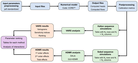
Figure 1.
Flowchart of the methodology used in this study.

Table 1.
Ranges and statistical distributions of the input parameters.
2.2. Site Description
The study area is located in Sabiñánigo (Huesca, Spain) where a lindane-producing factory INQUINOSA (Sabiñánigo, Spain) operated from 1975 to 1992 on the right bank of the Gállego River, which flows in a north/south direction (Figure 2). The Sabiñánigo dam was built in 1963 to provide hydroelectric power to chemical factories [38]. INQUINOSA (Sabiñánigo, Spain) deposited solid and liquid hexachlorocyclohexane (HCH) wastes in an uncontrolled manner in the Sardas landfill until approximately 1984 [39]. The landfill is located on the left bank of the Gállego river at 500 m from the Sabiñánigo reservoir.
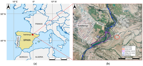
Figure 2.
(a) Location of the study area; (b) enlargement showing the model domain, the Sabiñánigo reservoir, the Sardas landfill, the Gállego River course, and the INQUINOSA (Sabiñánigo, Spain) former production site. The arrows along the Gállego River course indicate the flow direction.
The floodplain of the Gállego River downstream of the Sardas landfill is heavily affected by HCH wastes. By the 1980s, the Sardas landfill was completely filled with urban, construction, and industrial solid wastes including lindane production wastes (between 3 × 10⁴ and 8 × 10⁴ tons of solid HCH wastes) [39]. Since the landfill lacks a bottom liner system [39], DNAPL and leachates flowed freely from the landfill into the alluvial of the Gállego river until 1995. In addition, during the construction of road N-330 in the early 1990s, 5 × 10⁴ m3 of landfill waste was deposited on the ground surface of the alluvial plain [40]. In 1995, the landfill was sealed superficially with a PEAD sheet and laterally with a front slurry wall. However, the slurry wall does not prevent leachates from flowing into the alluvial aquifer [38,41].
The alluvial of the Gállego river consists of quaternary silts overlying a layer of sand and gravel. The Larrés marls underlie the quaternary sediments of the Gállego river alluvial [40]. A geological profile across the Sabiñánigo reservoir and the Gállego river floodplain was presented by Sobral et al. [38] (Figure 3). The sand and gravel are much more permeable than the silt and the marl [42].
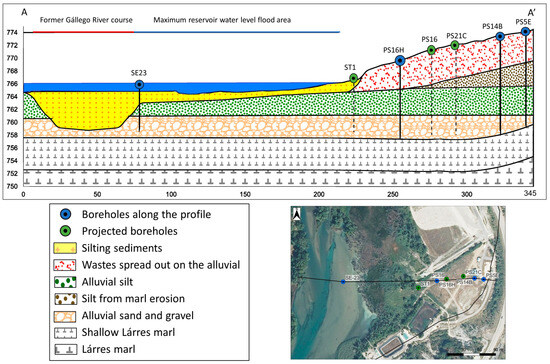
Figure 3.
Cross-sectional geological profile of the Sabiñánigo reservoir and the Gállego River alluvial plain as reported by Sobral et al. [38]. Alluvial deposits include a shallow silt layer (green) and a deep layer of sand and gravel.
Liquid HCH wastes were detected downstream of the Sardas landfill in 2009 [37], prompting hydrogeological and chemical studies aimed at identifying groundwater contaminant sources and proposing treatment options [39]. DNAPL has migrated by gravity through the alluvial due to its high density [43] and is mainly located on top of the marl layer [42] and inside its fractures [44]. This poses a significant risk since the aquifer and the reservoir are partially connected [38].
The layer of alluvial sands and gravels is confined by quaternary alluvial silts. Since its construction, the reservoir has undergone a siltation process [45] which deposited silting sediments and reducing greatly the reservoir capacity [38]. The alluvial silts and silting sediments act as an aquitard and play the role of a barrier for pollutants by retaining and slowing the arrival of contaminants to the reservoir [38]. However, the presence of DNAPL and HCH sorbed in the soil [42] constitutes a persistent source of organic pollutants.
2.3. Conceptual Model
The groundwater flow model presented here focuses on the alluvial aquifer downstream of the Sardas landfill with a large presence of solid and liquid HCH wastes. According to the monthly chemical analyses by the Ebro River Authority, the Sabiñánigo reservoir is the main receptor of chlorinated organic contaminants in the Sardas site.
The model assumes that the aquifer recharges through rainfall infiltration, from the surrounding fluvioglacial terraces on the right bank and from the Larrés marls on the left bank (Figure 4). The hydraulic conductivity of the sand and gravel layer is extremely large compared to that of the silts, silting sediments, and marl formations. Therefore, groundwater flow takes place mostly through the sand and gravel of the alluvial and discharges into the Gállego river, the Sabiñánigo reservoir, and underneath the Sabiñánigo dam in the downstream part of the study area. The tidal effect caused by the reservoir water level fluctuations has a significant effect on water transfer between the alluvial aquifer and the reservoir [38,46]. Aquifer groundwater flows from the aquifer into the reservoir for normal and low reservoir water levels. However, the flow reverses when the reservoir level rises above the piezometric head in the aquifer [38]. The sand and gravel located underneath the Sabiñánigo reservoir are assumed to be confined by the reservoir silting sediments and the alluvial silts.
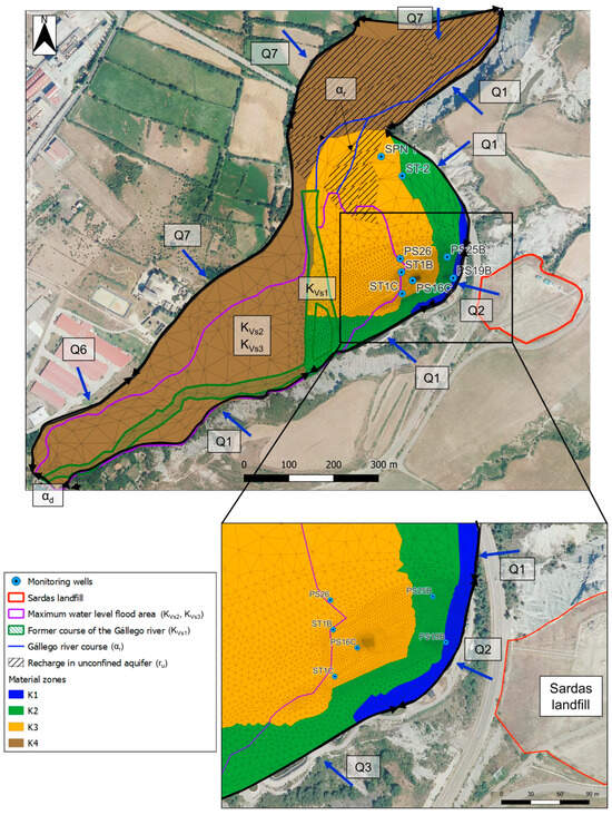
Figure 4.
2D finite element mesh, monitoring wells, material zones, boundary conditions, and GSA input parameters (top plot) and enlargement showing the area downstream of the Sardas landfill (bottom plot). The confined storage coefficient (SS) is the same in the four material zones. The sands and gravels are assumed to be confined in the alluvial (rc), except in the wooded areas (ru). Unconfined areas are shown with a back-hashed polygon.
2.4. Numerical Groundwater Flow Model
The numerical model presented here is an updated version of the groundwater flow model through the Gállego alluvial aquifer reported by Sobral et al. [38]. Contour maps of the thickness of the geological formations were slightly improved by incorporating information from recently drilled wells. Leakage coefficients for the aquifer/reservoir interactions were also updated.
The limits of the model domain include the right bank of the Gállego river along the west, the left bank of the river where the Sardas landfill is located, and the Sabiñánigo dam. The northern limit is located about 500 m north of the tail of the Sabiñánigo reservoir (Figure 4). The model was performed with a non-uniform finite element mesh of triangular elements made of 4399 nodes and 8655 elements (Figure 4). Groundwater flow simulation spans 109 days, starting on 15 July 2020 and ending on 31 October 2020. Time increments are all equal to 30 min. This time increment is equal to the frequency of the automatic reservoir level measurements.
Aquifer inflows include recharge from rainfall infiltration which was estimated with a hydrological water balance model [47], and inflows along the boundaries in both left and right banks. These inflows were simulated with a Neuman condition [38]. River/aquifer, reservoir/aquifer, and aquifer/dam interactions were simulated with Cauchy conditions as described by Sobral et al. [38].
2.5. Global Sensitivity Methods
2.5.1. Graphical Methods
Graphical methods provide a simple, compact, and informative tool to study global sensitivities. They are especially adequate for communicating results. They provide a good compromise between the complexity of other methods and compactness [48]. Two-variable interaction plots are helpful to identify visual parameter interactions.
The method of Cumulative Sum of the Normalized Reordered Model Output (CUSUNORO) curve plots condenses in a compact form the sensitivity of an output, , to a set of input parameters [18]. The CUSUNORO curve function, , is the scaled cumulative sum of the ordered residuals of the output, , [18] and is given by:
where and are the sample mean and standard deviation of the outputs, respectively, is the sample size or the number of simulations, and is the j-th ordered residual. The function can be interpreted based on the following terms: (1) A divisor term or scaling factor, , which guarantees that the cumulative sum is scaled relative to the sample size n; (2) A divisor term (standard deviation) which ensures that z(i) is dimensionless and standardized; and (3) A summation term representing the cumulative sum of the deviations of the ordered output values from the mean .
2.5.2. Sobol Method
The High Dimensional Model Representation (HDMR) method evaluates the input-output relationships of complex models with many input parameters [22]. The Sobol method for global sensitivity analysis requires to compute complex quadratures in a high dimensional space. Random and quasi-random rules are usually applied, which involve a set of sample points where model outputs are analyzed. The Sobol sequence was selected for this study [49]. The input parameters are normalized to range from zero to one.
The variance of the output is split as the sum of non-negative variance terms, each associated with combinations of input parameters [22]. Sobol indexes quantify the combined contributions of the input parameters to the variance of the output. The first-order sensitivity index or “main effect” index, , measures the relative individual contribution of the -th input variable on the variance of the output. The second-order sensitivity indexes, , measure the interactions between the -th and the -th inputs on the output variable [22]. Both terms, and , are usually provided by HDMR software packages. The total sensitivity index, or total-effect index or total-order index, , is a measure of the total contribution of the -th input to the output variance [50,51], including all the interactions with the rest of the inputs of order ranging from 2 to . Its expression is given by:
2.5.3. Variogram Analysis of Response Surfaces
The variogram analysis of response surfaces (VARS) is a method of characterizing the structure and variability of model outputs within the input parameter space [27]. VARS computes several global sensitivity metrics, including Morris and total sensitivity Sobol indexes by using a tailored sampling strategy [27]. VARS star-based sampling strategy requires all input parameters to be normalized to range between zero and one. Then, the star centers are selected by using a random sampling strategy. A cross-section of equally spaced points with a selected resolution Δh is performed for each star center and for each input variable. Each set of points constitutes a “star”. There are different methods to sample the star centers [52]. The Halton sequence was selected for this study [53]. The outputs are calculated at all points for all stars. Directional variograms and covariograms are calculated along the lines of the input parameters.
Like other GSA methods, VARS requires performing a sufficiently large number of model simulations to obtain estimates of the directional variograms for each input variable. The variograms along the directions of the parameters provide the sensitivity indexes of the GSA. The limit of the directional variogram divided by h2 as h approaches 0, corresponds to Campolongo’s version of the Morris effects [28]. On the other hand, the limit of the variogram for large h corresponds to the total variance linked to the Sobol total effect or total sensitivity index [27].
The Morris and Sobol methods are limiting cases of VARS. The directional variograms of VARS provide metrics that accurately estimate Sobol and Morris indexes [27]. In addition, VARS calculates the Integrated Variogram Across a Range of Scales index (IVARS50). IVARS50 provides a sensitivity index corresponding to intermediate scales and is calculated from the directional variograms according to:
where is the directional variogram and is the normalized input parameter. It should be recalled that the VARS method requires that all the input parameters be normalized to range from zero to one.
2.6. Inputs and Outputs
Input parameters were selected based on the conclusions of the local sensitivity analyses performed by Sobral et al. [38]. The final list of parameters includes also other potentially relevant parameters such as boundary fluxes. The final list of input parameters considered in the GSA includes (Figure 4): (1) The hydraulic conductivities of the aquifer in four material zones which were defined to account for the spatial heterogeneity of the alluvial aquifer (K1, K2, K2 and K4); (2) The aquifer specific storage (SS); (3) The vertical hydraulic conductivities of the aquitard interposed between the aquifer and the reservoir which includes the silting sediments settled along the former course of the Gállego river (KVs1), the silting sediments in the rest of the reservoir (KVs2) and the alluvial silts (KVs3); (4) The leakage coefficients of the aquifer/river interactions (αr) and the conductance for the flow underneath the dam (αd); (5) Aquifer recharge rates from precipitation in confined (rc) and unconfined (ru) parts of the aquifer; and (6) Boundary inflows (Q6, Q7, Q9, Q2 and Q1). The ranges and statistical distributions of the input parameters are listed in Table 1. Log-uniform probability density functions were used for the hydrodynamic parameters and leakage coefficients, and uniform distributions were adopted for recharge rates and boundary inflows (Table 1). GSA and geostatistical analyses often assume that hydrogeological parameters such as hydraulic conductivities, storage coefficients, and leakage coefficients follow log-normal distributions. Log-normal distributions ensure that simulated values are always positive and provide a more realistic representation of parameter variability and skewness compared to uniform distributions. On the other hand, boundary inflows and recharge rates usually vary within given ranges with all values equally probable, and thus, uniform distributions capture better their uncertainties without biasing the analysis toward specific values within the adopted ranges.
The hydraulic conductivities K1 to K4 in Table 1 do not correspond to the conductivities of aquifer layers. Instead, they correspond to the hydraulic conductivities of four material zones. The aquifer is divided into four portions (here denoted as material zones). All material zones have the same value of the specific storage, SS. However, these zones have different hydraulic conductivities (K1 to K4). Even though these hydraulic conductivities have the same statistical properties, they vary independently from one another.
The outputs of the GSA were selected to gain insight into the sensitivity of model calibration metrics to changes in input parameters and evaluate the time change in sensitivities of hydraulic heads, h, aquifer/reservoir fluxes, Q, and Darcy velocity, q, caused by the tidal effects. The outputs related to calibration metrics include the global mean absolute error in hydraulic heads (MAEg), the global root mean square error in hydraulic heads normalized by the standard deviation of the measured head data (NRMSEg), and the global Nash–Sutcliffe index [54] (NSEg) of the head residuals (measured minus computed heads) at 8 monitoring wells (Figure 5). Other outputs include the computed piezometric heads in wells ST1C, PS19, and SPN1 at three selected times, t1, t2, and t3, which correspond to an event of sudden rise of the reservoir water level that took place from 18 September 2020 at 20:30 to 19 September 2020, at 04:30 (Figure 6). The heads in these three wells at the three selected times are denoted as ST1Ct1, ST1Ct2, ST1Ct3, PS19Bt1, PS19Bt2, PS19Bt3, SPN1t1, SPN1t2, and SPN1t3. Other outputs include the aquifer/reservoir fluxes at times t1, t2, and t3, which are denoted as Qt1, Qt2, and Qt3, and the average modulus of the Darcy velocity near well PS16C where a tracer test was performed (qav).
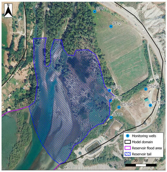
Figure 5.
Map showing the reservoir tail area (hashed blue polygon) where aquifer/reservoir fluxes were calculated at times t1, t2, and t3, the monitoring wells whose piezometric data were used to calculate the calibration metrics, monitoring wells ST1C, PS19B, SPN1, and PS16C (where the average Darcy velocity is computed).
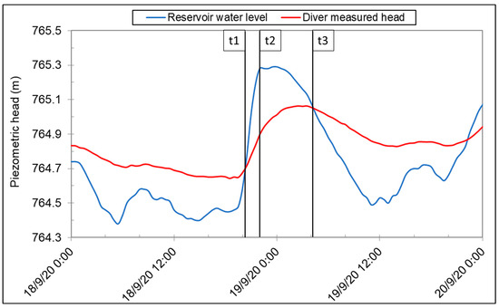
Figure 6.
Measured reservoir hydrograph and piezometric heads in well ST1C from 18–20 September 2020. The computed piezometric heads in monitoring wells ST1C, PS19B, and SPN1 and the aquifer/reservoir fluxes are analyzed at the following times: (1) t1, 18 September 2020, 20:00 (low reservoir water level), (2) t2, 18 September 2020, 22:30 (peak reservoir water level) and (3) t3, 19 September 2020, 04:30 (descending reservoir water level).
The model head residuals were calculated as the differences between measured and computed heads using recorded piezometric head data from ST1B, ST1C, ST2, SPN1, PS16C, PS19B, PS25B, and PS26 wells. The mean absolute error (MAE), the root mean squared error normalized by the standard deviation of the measured data (NRMSE), and the Nash–Sutcliffe index (NSE) were computed for each well (). The metrics were globalized to evaluate the goodness of fit in the eight wells equipped with divers:
where:
- is the number of monitoring wells.
- is the number of measured piezometric heads in the -th well.
- is the total number of measured piezometric heads in all the wells.
- is the standard deviation of the measured piezometric heads in the -th well.
- , and are the mean absolute error, the root mean squared error, and the Nash–Sutcliffe index for the -the well.
- is the standard deviation of the measured piezometric heads in all wells.
2.7. Global Sensitivity Simulation Runs
Global sensitivity simulation runs were generated by using two different sequences. A first set of 30,800 runs was prepared for VARS by using the Halton sequence to generate the sequence of star centers [53]. The second sequence of 16,384 runs was obtained by using the Sobol method [49]. The runs were performed at the Galician Supercomputing Center (CESGA).
2.8. Software
Model simulations were performed with CORE2DV5, a two-dimensional (2D) finite element code for transient saturated and unsaturated water flow, heat, and multicomponent reactive solute transport in heterogeneous and anisotropic porous and fractured media [55]. The code solves for groundwater flow and heat and solute transport by using Galerkin triangular finite elements and an Euler time discretization scheme. CORE2D V5 has undergone extensive verification against analytical solutions and has been benchmarked against other groundwater flow and reactive transport codes [56,57]. CORE2DV5 has been used extensively for modeling groundwater flow and solute transport in aquifers and lab and in situ experiments [58,59].
The single processor code CORE2DV5 was compiled at the CESGA by using the FinisTerrae-III supercomputer [60,61]. This advanced computing infrastructure supports the concurrent execution of hundreds of simultaneous and parallel model runs. The simulation of the VARS-Halton and Sobol sequences runs took 6 days of computing wall time. The same task would have taken more than three years running on a personal computer.
VARS version 2.1 was run under MATLAB® version 2022a in an UBUNTU 20.04.6 LTS system. HDMR computations were carried out by using both SALib [62] and GUI-HDMR V1.1 [63].
3. Results and Discussion
3.1. Groundwater Flow Model Results
The computed hydraulic gradient at the Sardas site downstream of the landfill is very small due to the large hydraulic conductivity of the layer of sand and gravel, and the small groundwater inflows [38]. The reservoir water level fluctuates daily with an amplitude of about 1 m and a period of 12 h. The daily fluctuations of the reservoir water level induce a tidal effect on the piezometric heads of the aquifer because the reservoir and the aquifer are hydraulically connected. This tidal effect is like a sea tide in a costal aquifer. The average water level in the reservoir (764.80 m) is slightly smaller than the piezometric head in the aquifer (764.90 m). Groundwater generally flows from the aquifer to the silting sediments and the alluvial silts of the reservoir. However, when the reservoir water level rises above the piezometric head in the aquifer, the Sabiñánigo reservoir recharges the aquifer, resulting in a rise in piezometric heads. The modulus of the Darcy velocity in the aquifer decreases during these high-reservoir water level events. If the duration of the high water level is long enough, the direction of groundwater flow near the reservoir may reverse [38,41]. Later, groundwater recovers its original direction when the piezometric head in the alluvial rises above the reservoir water level or the reservoir water level decreases bellow the piezometric head in the aquifer. Aquifer piezometric head, groundwater flow direction, and discharge flow to the silts and silting sediments are strongly affected by the oscillation of the water level in the Sabiñánigo reservoir.
The fluctuations of the piezometric head in the aquifer are damped and delayed compared to the oscillations of the reservoir water level because the aquitard acts as a dumping barrier between the reservoir and the aquifer [38]. The amplitude of the oscillations of the piezometric heads, Ah, and the time lag, tR, are very sensitive to the specific storage coefficient of the layer of sands and gravels (SS), and the vertical hydraulic conductivities of the aquitard (KVs1, KVs2 and KVs3) [38].
3.2. GSA Results for the Groundwater Flow Model of the Gállego Alluvial Aquifer
3.2.1. Graphical Results
Two-variable scatterplots are useful to identify and illustrate the interactions of two input parameters. Figure 7 shows two-variable scatterplots of the computed heads in three monitoring wells (outputs ST1Ct2, PS19Bt2, and SPN1t2) and the aquifer/reservoir flow (Qt2) at time t2 corresponding to the peak reservoir water level. The outputs are plotted versus the vertical conductivity of the aquitard (KVs1). These plots correspond to the 16 384 runs of the Sobol sequence. The clouds of plots are shown for the following three ranges of percentiles, p, of the specific storage coefficient (SS): (1) p < 30%; (2) 30% < p < 70%, and (3) p > 70%.
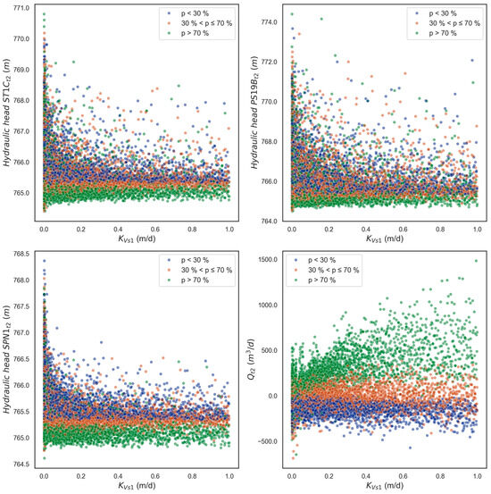
Figure 7.
Scatterplots of the computed piezometric heads in wells ST1Ct2 (upper left plot), PS19Bt2 (upper right plot), SPN1t2 (lower left plot), and Qt2 (lower right plot) versus the vertical hydraulic conductivity of the silting sediments in the former river course (Kvs1). The sample of 16384 points was generated with a Sobol sequence. The clouds of plots are shown for the following three ranges of percentiles, p, of the specific storage coefficient (SS): (1) p < 30%; (2) 30% < p < 70%, and (3) p > 70%.
The scatterplots show that the computed heads and the aquifer/reservoir flow at time t2 depend on SS. Generally, the computed piezometric heads in wells ST1C and SPN1 at t2 are low for large SS (p > 70%). However, simulations corresponding to extreme values of other input parameters result in high piezometric heads even for high values of SS. On the other hand, the computed heads are higher when SS is in the lower percentile (p < 30%). It should be noticed that the well PS19B is located further away from the reservoir, and thus, its piezometric head is less affected by the interaction between KVs1 and SS.
The scatterplot of Qt2 shows three branches. The most negative flows, which correspond to aquifer discharge into the reservoir, at time t2 are associated with low values of SS (p < 30%) while the largest positive water flows (flow from the reservoir into the aquifer) occur for high SS values (p > 70%). The water flow oscillates from positive (aquifer recharge) to negative (aquifer discharge) for intermediate values of SS (30% < p < 70%). The amplitude of the oscillations of the piezometric heads in the aquifer, Ah, is inversely proportional to the value of the specific storage of the aquifer. When SS is low, Ah is large and the piezometric heads in the alluvial oscillate strongly and rise above the reservoir water level, thus leading to groundwater discharge to the reservoir. On the other hand, when SS is large, Ah is small because the piezometric heads increase more slowly. In this case, the piezometric heads remain below the reservoir water level during the events of rise of the reservoir water level, thus, leading to flow from the reservoir into the aquifer.
Figure 8 and Figure 9 show CUSUNORO curves for computed heads in wells ST1C, PS19B, and SPN1 at times t1, t2, and t3 and MAEg, NRMSEg, NSEg, Qt1, Qt2, Qt3, and qav.
From the CUSUNORO curves above, parameters K3 (green), Q2 (red), and K2 (orange) consistently exhibit the highest maximum absolute values across all hydraulic head plots, except for the hydraulic head at well SPN1, where parameters αr (yellow), KVs1 (brown) and Ss (purple) are more influential. Q6 (blue) and K1 (blue) typically show the lowest maximum absolute values. The most influential parameters across all performance metrics (MAEg, NRMSEg, and NSEg) are K3, Q2, K2, and αr. Q6 and Ss exhibit lower values. Parameters αr, KVs1, and Q2 have the largest influence on the aquifer/reservoir fluxes except at time t2, Qt2. At time t2, Ss is the most influential parameter. Again, Q6 and K1 consistently show the smallest influences.
Q2, K3, and K2 have the highest influence on the average groundwater Darcy velocity modulus near well PS16C, while Q6 and Ss are the least influential parameters for this output.
Most of the CUSUNOTO curves do not show crossings of the x-axis. This attests to the expected monotonicity of the outputs versus the input parameters. Some crossings of the x-axis are found in the curves of the least influential parameters, especially for Q6 and K1.
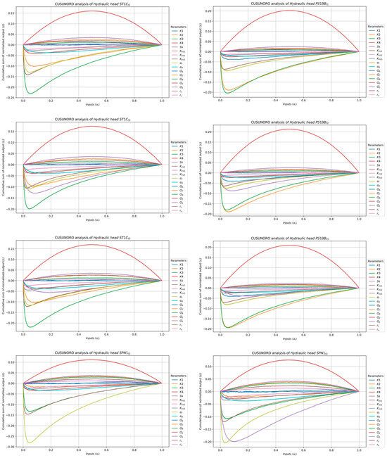
Figure 8.
CUSUNORO curves of computed head in wells ST1C and PS19B at times t1, t2 and t3; and well SPN1 at times t1 and t2.
Figure 8.
CUSUNORO curves of computed head in wells ST1C and PS19B at times t1, t2 and t3; and well SPN1 at times t1 and t2.
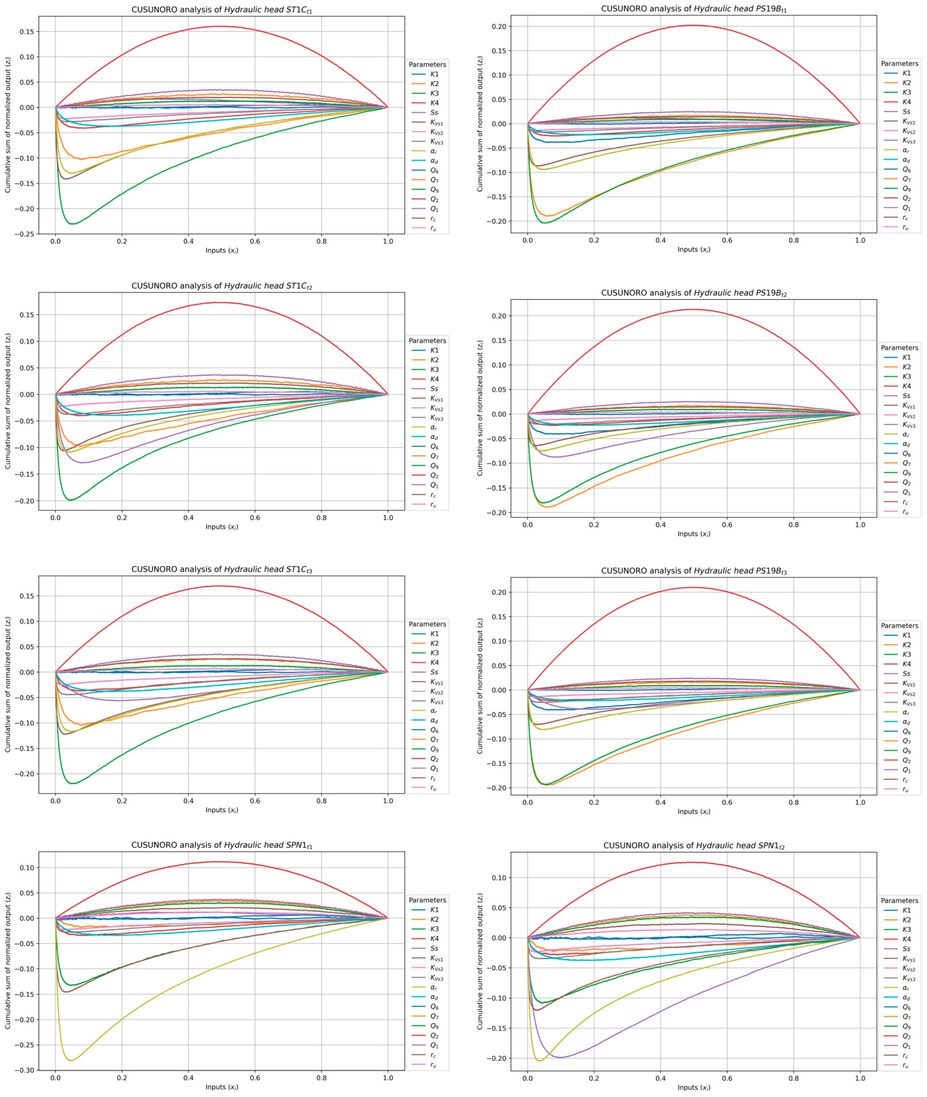
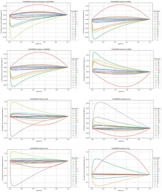
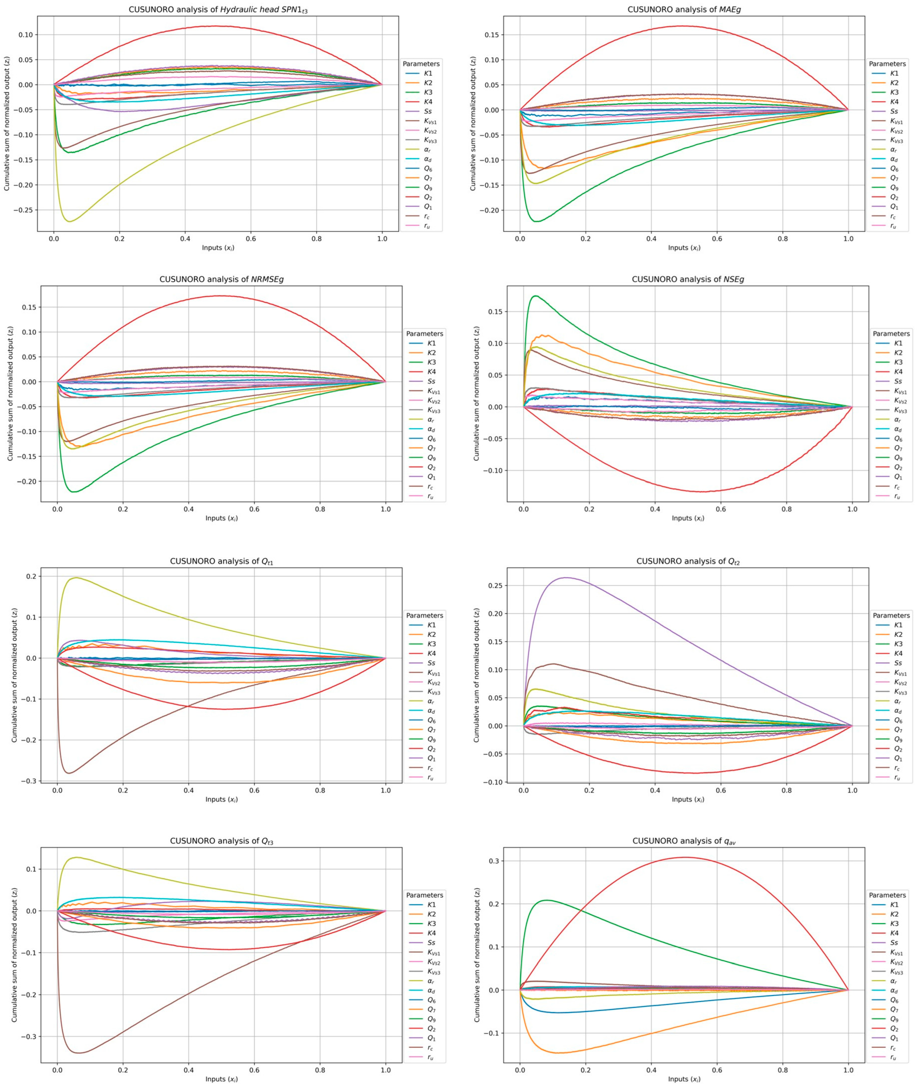
Figure 9.
CUSUNORO curves of the computed head in well SPN1 at time t3, MAEg, NRMSEg, NSEg, Qt1, Qt2, Qt3, and qav.
Figure 9.
CUSUNORO curves of the computed head in well SPN1 at time t3, MAEg, NRMSEg, NSEg, Qt1, Qt2, Qt3, and qav.
3.2.2. VARS Results
Figure 10 and Figure 11 show the IVARS50 indexes for the global mean absolute error (MAEg), and the average groundwater Darcy velocity modulus (qav) as a function of the number of star centers. They also show the ranking of the input parameters and the robustness of the ranking. It should be noticed that IVARS50 achieves stable values after just 50 star centers, which amounts to 7700 runs. The largest sensitivity indexes for MAEg correspond to the aquifer hydraulic conductivity in material zone 3 (K3), the boundary inflow Q2 which corresponds to groundwater flow coming from the Sardas landfill, the vertical conductivity of the silts (KVs1) and the aquifer/river conductance (αr). IVARS50 of the Darcy velocity, qav, is largest for Q2, K3, and K2. The rest of the parameters have much smaller indexes.
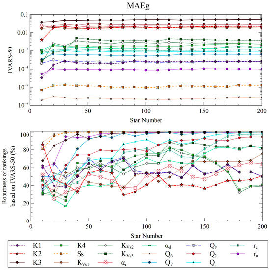
Figure 10.
IVARS50 indexes of input parameters as a function of the number of star centers for MAEg (upper plot), and robustness of ranking as a function of the number of star centers (bottom plot).
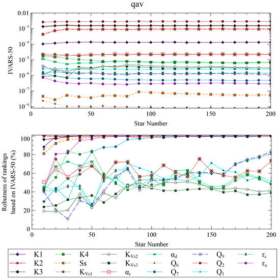
Figure 11.
IVARS50 indexes of input parameters as a function of the number of star centers for the average Darcy velocity (qav) (upper plot), and robustness of ranking as a function of the number of star centers (bottom plot).
The robustness of ranking of input parameters K2, K3, SS, ru, and Q7 for both outputs is greater than 90% after 50 stars. However, for the rest of the input parameters, the robustness is smaller than 80%, and, sometimes, not stable even after 200 stars. Input parameters αr and KVs1 are very influential for MAEg, but they show a robustness measure that ranges from 50 to 70% after 100-star centers. Robustness does not directly increase with the number of star centers for some input parameters. This could be caused by interactions among SS, aquitard vertical conductivity KVs1, and aquifer/river conductance αr at some water level rise events. Another reason for the lack of stability in the robustness of rankings is that the least relevant input variables interfere with the calculation of sensitivity indexes of the most relevant parameters. However, the rankings of the most and the least significant input parameters are stable with just 50-star centers (7700 runs). Input parameters with intermediate influence are also well identified, despite not being ranked reliably.
Sample variograms along the directions of the 17 input parameters were computed for the piezometric heads in wells ST1C, PS19B, and SPN1 at times t1, t2, and t3, the calibration metrics, the aquifer/reservoir fluxes at times t1, t2 and t3 and the average groundwater Darcy velocity modulus near well PS16C. Only a limited number of parameters are relevant for each output variance. Figure 12 and Figure 13 show the sample variograms along the directions of the five most influential parameters. VARS-TO, IVARS50, and VARS-ABE metrics are computed from the variograms. Figure 14 and Figure 15 show the VARS-ABE, IVARS50, and VARS-TO indexes for each output considering all the input parameters.
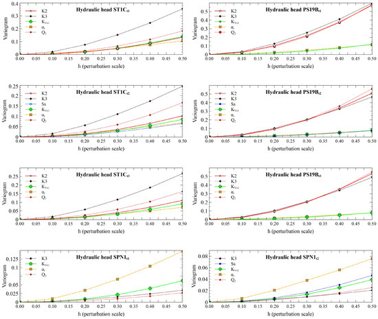
Figure 12.
Sample variograms of the computed heads in monitoring wells ST1C and PS19B at times t1, t2, and t3 and monitoring well SPN1 at times t1 and t2. Only the variograms of the five most influential parameters are shown in the plots.
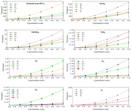
Figure 13.
Sample variograms of the computed head in well SPN1 at time t3, MAEg, NRMSEg, NSEg, Qt1, Qt2, Qt3, and qav. Only the variograms of the five most influential parameters are shown in the plots.
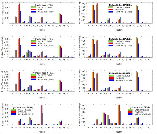
Figure 14.
VARS-TO, IVARS50, and VARS-ABE indexes for the computed heads in wells ST1C and PS19B at times t1, t2, and t3 and well SPN1 at times t1 and t2.
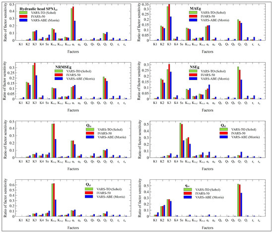
Figure 15.
VARS-TO, IVARS50, and VARS-ABE indexes for the computed head in well SPN1 at time t3, MAEg, NRMSEg, NSEg, Qt1, Qt2, Qt3, and qav.
The most influential parameters for the computed head in well ST1C at times t1, t2, and t3 are K3 and Q2, followed by KVs1, αr, and K2. The ranking in well PS19B is similar to the ranking in well ST1C. However, the sensitivity indexes of K3, K2, and Q2 in well ST1C are much larger than those of well PS19B. K3 is much more relevant than K2 in well ST1C while K2 and K3 have almost similar sensitivity indexes in well PS19B. The sensitivity indexes of the hydraulic conductivities depend on the location of the wells. Material zone 3 is the largest zone of the Sardas site. Material zone 2 is located between material zones 1 and 3. Material zone 1 is much smaller than the other two and is located just downstream of the Sardas landfill. KVs1 is more influential for the head in well ST1C than for the well PS19B. ST1C is located right next to the reservoir’s maximum flood area and PS19B is located 135 m to the east of the reservoir. Tidal effects on the aquifer depend on the duration of the high reservoir level, its amplitude, and the distance to the reservoir. Likewise, the head in well PS19B is most sensitive to Q2 because this well is near the boundary just downstream of the Sardas landfill.
The sensitivity indexes for the computed heads in well SPN1 differ from those of other monitoring wells because well SPN1 is near the Gállego riverbed. αr is the most influential parameter in well SPN1 followed by KVs1.
Despite not being an influential input, the relevance of SS for the computed heads in the monitoring wells increases from time t1 (low level) to time t2 (peak reservoir water level). The sensitivity indexes of SS decrease when the reservoir water level descends at time t3. The time change of the sensitivity of SS in well SPN1 is more significant than in wells ST1C and PS19B.
The most influential parameters for the calibration metrics (MAEg, NRMSEg, and NSEg) are K3, K2, and Q2, followed by KVs1 and αr. Most of the monitoring wells are located in material zones 2 and 3 and near the boundary zone corresponding to Q2. Aquifer/reservoir and aquifer/river interactions affect the computed head gradient, tR, and Ah. SS only affects the temporal variability of computed heads and not their average values. Since calibration metrics evaluate the average fit of the computed heads in the monitoring wells, the relevance of SS for the calibration metrics is very low compared to its relevance on the computed heads at specific times. SS is especially relevant during events of sudden rise of the reservoir water level.
To facilitate the interpretation of the sensitivities of reservoir/aquifer fluxes (Qt1, Qt2, Qt3), one should recall that the silting sediments (KVs1 and KVs2) are more permeable than alluvial silts (KVs3). Groundwater discharges mainly through the former course of the Gállego River, where only silting sediments confine the aquifer (KVs1). If the aquifer is less connected to the Gállego River (lower values of αr), groundwater discharges to the reservoir. On the other hand, if the aquifer and the river are more connected (higher values of αr), groundwater discharges to the reservoir and the river. As expected, the greater the inflow of water from the landfill (Q2), the more groundwater is discharged to the reservoir.
The aquifer/reservoir groundwater flow changes with time due to the reservoir tidal effect. The most influential parameters for the aquifer/reservoir groundwater flow are also time-dependent. KVs1 is the parameter with the largest sensitivity index at time t1 when the reservoir water level is low. The second influential parameter is the aquifer/river leakage coefficient, αr. The boundary inflow Q2 is the third most relevant parameter. However, when the reservoir water level rises suddenly rises at time t2, the parameter sensitivities change. The most influential parameter becomes SS followed by KVs1. We recall that in the model reference run [38], there is flow from the reservoir into the aquifer when the reservoir water level rises above the piezometric head in the aquifer. If the specific storage of the aquifer is high, a larger part of the flow coming from the reservoir is stored in the aquifer, which results in a smaller rise of the piezometric head in the aquifer.
The reservoir flood area depends on its water level, so when the water level rises at time t2, the area where the alluvial silts confine the aquifer underneath the reservoir increases. The areas of the reservoir away from the former course of the Gállego River are assumed to be confined by both silting sediments (KVs2) and alluvial silts (KVs3). The relevance of KVs3 increases slightly when the reservoir floods more parts of the alluvial, but its relevance is still much smaller than those of KVs1 and SS. When the water level of the reservoir descends at time t3, the parameter sensitivities tend to be similar to those of Qt1. For Qt3, the sensitivity of KVs1 is much larger than those of αr and Q2. The sensitivity of SS remains, but it is much less relevant than for Qt2,
The most influential parameters for the average modulus of the Darcy velocity (qav) near well PS16C are Q2, K3, and K2. K1 is slightly relevant, and the contribution of the rest of the parameters is negligible. The Darcy velocity in the aquifer mainly depends on the boundary inflow Q2 because this well is located in material zone 3 and near the boundary downstream of the Sardas landfill.
The sensitivity indexes of SS are time-dependent for the computed heads in the wells, and the aquifer/reservoir fluxes (Figure 16). When the reservoir water level rises above the piezometric head in the aquifer at time t2, the reservoir starts recharging the aquifer, and the piezometric head in the alluvial starts rising. If the specific storage is small, the amplitude of the oscillation of the piezometric head increases. This affects especially the aquifer/reservoir fluxes (Qt1, Qt2 and Qt3). The sensitivities of the computed head in well SPN1, located near the Gállego river, are largest for αr and KVs1 and SS at time t2.
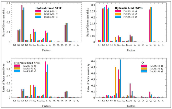
Figure 16.
IVARS50 sensitivity indexes for computed heads in wells ST1C (top left plot), PS19B (top right plot), and SPN1 (bottom left plot) and aquifer/reservoir flow (bottom right plot) at times t1, t2, and t3.
On the other hand, well ST1C is closest to the reservoir and further away from the Gállego River. In this well the sensitivity index of SS is smaller than in well SPN1. Finally, the sensitivity of the head in well PS19B to SS is irrelevant because the well is far away from the Gállego River and the reservoir flood area.
The IVARS50 sensitivity indexes for calibration metrics, MAEg, NRMSEg, and NSEg are very similar (Figure 17). The most influential parameters are the same for all the metrics. The rankings show some slight differences. Input ranking for the MAEg is K3, Q2, αr, K2, and KVs1, while αr and K2 switch places for NRMSEg and NSEg. NRMSEg and NSEg are more prone to the presence of outliers because their formulas include squared residuals.
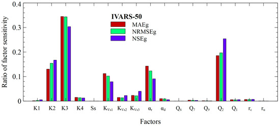
Figure 17.
IVARS50 sensitivity indexes for calibration metrics MAEg, NRMSEg, and NSEg.
Sensitivity indexes are large for K3, Q2, αr, K2, and KVs1. Some input variables have very small sensitivity indexes.
3.2.3. HDMR Results and Analysis of Interactions for the Sobol Sequence
Tables S1–S23 in the SM show the values of the first order (main effects), Si, and 2nd order effects, Sij, calculated with SALib [62] and GUI-HDMR [63] and the parameter ranking for (1) The computed piezometric heads in wells PS19B, SPN1, and ST1C at times t1, t2, and t3; (2) The global mean absolute error (MAEg); (3) The global Nash–Sutcliffe index (NSEg); (4) The global normalized root mean squared error (NRMSEg); (5) The average groundwater Darcy velocity modulus near well PS16C (qav); and (6) The computed aquifer/reservoir fluxes at times t1, t2, and t3 (Qt1, Q t2 and Qt3) by using 16 384 runs.
HDMR lower bound estimates for the total effects, (Si + Sij), are compared to the VARS intervals of the total effects for each parameter. SALib and GUI-HDMR indexes generally agree although they show some small differences. The analysis of the interactions among parameters is an important part of the global sensitivity analysis. Interactions represent the joint influence of parameters on the model outputs. Usually, interactions are revealed when the sum of Sobol’s first-order indexes is significantly smaller than one.
In the next paragraphs, the Sobol-based lower bound estimates for the total effects will be denoted simply as “total effects” to shorten the presentation of the HDMR results. The largest main effect, Si, for the piezometric head in well ST1C at time t1 is equal to 0.242 and corresponds to K3 (see Table S1 in Supplementary Materials). The sum of Sobol’s first-order indexes is equal to 0.644. The total effects of the piezometric head in well ST1C at time t1 are slightly larger than one (see Table S1 in Supplementary Materials). Second-order effects for this output are important especially due to the interaction between K3 and K2. Interactions of smaller relevance occur between Q2 and K3, between KVs1 and αr, and between Q2 and K2. Sobol total effects STi are typically larger and fall outside the ranges of the VARS total effects.
The largest main effect, Si, of the piezometric head in well ST1C at time t2 is equal to 0.194 and corresponds to K3 (see Table S2 in Supplementary Materials). The sum of Sobol’s first-order indexes is equal to 0.628. The total effects of the piezometric head in well ST1C at time t2 are slightly larger than one (see Table S2 in Supplementary Materials). Second-order effects here are relevant especially due to the interaction between Q2 and K3. There are also interactions of smaller relevance between K3 and K2, between KVs1 and αr, and between Q2 and K2. Sobol total effects STi and those of VARS generally agree although they show some discrepancies, especially for the K1 and ru.
The largest main effects, Si, for the piezometric head in well ST1C at time t3 correspond to K3 and Q2 (see Table S3 in Supplementary Materials). The sum of Sobol’s first-order indexes is equal to 0.644. The total effects of the piezometric head in well ST1C at time t3 are equal to 1.223 (see Table S3 in Supplementary Materials). Second-order effects for this output are relevant due to interactions of K3 with K2 and Q2, and KVs1 with αr. The Sobol total effects STi generally fall within the intervals of VARS total effects.
The largest main effects, Si, for the piezometric head in well PS19B at time t1 correspond to Q2, K3, and K2 (see Table S4 in Supplementary Materials). The sum of Sobol’s first-order indexes is equal to 0.71. The total effects STi for the piezometric head in well PS19B at time t1 are slightly greater than one (see Table S4 in Supplementary Materials). Second-order effects here are relevant especially due to the interactions among Q2, K3, and K2. The total effects of STi fall within the intervals of VARS total effects.
The largest main effects for the piezometric head in well PS19B at time t2 correspond to Q2, K2, and K3 (see Table S5 in Supplementary Materials). The sum of Sobol’s first-order indexes is equal to 0.699. The total effects STi for the piezometric head in well PS19B at time t2 are slightly greater than one (see Table S5 in Supplementary Materials). Second-order effects for this output are important especially due to the interaction between Q2 and K2. There are also interactions of smaller relevance between Q2 and K3, between K3 and K2, and between αr and KVs1. The Sobol total effects STi are typically larger and fall outside the ranges of the VARS total effects.
The largest Si for the piezometric head in well PS19B at time t3 corresponds to Q2. K2 and K3 are in second and third position (see Table S6 in Supplementary Materials). The sum of Sobol’s first-order indexes is equal to 0.703. Second-order effects for this output are important especially due to the interaction between Q2 and K2. There are also interactions of smaller relevance between Q2 and K3, between K3 and K2, and between αr and KVs1. The Sobol total effects STi are generally larger and out of the intervals of the VARS estimates.
αr shows the largest main effect, Si, for the piezometric head in well SPN1 at time t1 which is equal to 0.394. The second largest effect corresponds to KVs1 (see Table S7 in Supplementary Materials). The sum of Sobol’s first-order indexes is equal to 0.69. The total effects of the piezometric head in well SPN1 at time t1 are close to one (see Table S7 in Supplementary Materials). Second-order effects for this output are relevant especially due to the interaction between Q2 and K3. The Sobol total effects STi are overall higher and beyond the limits of the VARS estimates.
The largest main effects, Si, for the piezometric head in well SPN1 at time t2 correspond to αr and SS (see Table S8 in Supplementary Materials). The sum of Sobol’s first-order indexes is equal to 0.655. The total effects of the piezometric head in well SPN1 at time t2 are slightly larger than 1 (see Table S8 in Supplementary Materials). Second-order effects for this output are relevant especially due to the interaction between αr and KVs1. There are also smaller interactions of Q2 with K3 and with αr. The Sobol total effects are generally larger and out of the intervals of the VARS estimates.
The largest main effects, Si, for the piezometric head in well SPN1 at time t3 correspond to αr and K3 (see Table S9 in Supplementary Materials). The sum of the Sobol first-order indexes is equal to 0.679. The total effects of the piezometric head in well SPN1 t3 are close to 1 (see Table S9 in Supplementary Materials). Second-order effects are relevant mainly due to the interaction between αr and KVs1, and to a lower extent to the interactions of Q2 with K3 and αr. The Sobol total effects are generally larger and out of the intervals of the VARS estimates.
The largest main effects, Si, of the global mean absolute error correspond to K3, Q2, and αr (see Tables S10 and S11 in Supplementary Materials). The sums of Sobol’s first-order indexes calculated with SALib and GUI-HDMR are equal to 0.682 and 0.734, respectively. The total effect of the global mean absolute error computed with SALib is equal to that of GUI-HDMR (see Tables S10 and S11 in Supplementary Materials). Second-order effects for this output are important especially due to the interactions between Q2 and K3 and between K3 and K2. There are also interactions of smaller relevance between αr and KVs1 and between Q2 and K2. The SALib total effects STi fall within the intervals of VARS estimates or are slightly larger than VARS total effects.
K3 shows the largest main effect of the global normalized root mean squared error which is equal to 0.245 (SALib). The second largest effect corresponds to Q2 (see Tables S12 and S13 in Supplementary Materials). The sums of Sobol’s first-order indexes calculated with SALib and GUI-HDMR are equal to 0.675 and 0.731, respectively. The total effects of the global normalized root mean squared error are close to one (see Tables S12 and S13 in Supplementary Materials). Second-order effects for this output are relevant especially due to the interaction between K3 and K2, and between Q2 and K3. The total effects STi from SALib are either within the ranges of VARS estimates or slightly exceed the VARS total effects.
The largest main effect of the global Nash–Sutcliffe index corresponds to K3. Q2 and K2 are in the second and third positions (see Tables S14 and S15 in Supplementary Materials). The sums of Sobol’s first-order indexes calculated with SALib and GUI-HDMR are equal to 0.411 and 0.477, respectively. The total effect of the global Nash–Sutcliffe index computed with SALib is smaller than that of GUI-HDMR (see Tables S14 and S15 in Supplementary Materials). Second-order effects for this output are important especially due to the interaction between Q2 and K3. There are also interactions of smaller relevance between K3 and K2, between Q2 and K2, and between αr and KVs1. The SALib total effects STi fall within the intervals of VARS estimates or are slightly larger than VARS total effects.
The largest main effects of the computed aquifer/reservoir flux at time t1 correspond to KVs1 and αr (see Tables S16 and S17 in Supplementary Materials). The sums of Sobol’s first-order indexes calculated with SALib and GUI-HDMR are equal to 0.716 and 0.746, respectively. The total effects of the computed aquifer/reservoir flux at time t1 are close to one (see Tables S16 and S17 in Supplementary Materials). The second-order effects for this output are significant, particularly because of the interactions of KVs1 with αr, Ss, Q2, and K3. Additionally, there are less significant interactions between αr and K3, and between αd and K4. The Sobol total effects STi calculated by SALib are overall higher than the VARS estimates.
The largest main effect of the computed aquifer/reservoir flux at time t2 is equal to 0.362 (SALib) and corresponds to SS (see Table S18 in Supplementary Materials). The sums of Sobol’s first-order indexes calculated with SALib and GUI-HDMR are equal to 0.514 and 0.469, respectively. The total effects of the computed aquifer/reservoir flux at time t2 are greater than one (see Tables S18 and S19 in Supplementary Materials). For this output, the second-order effects are notable, mainly due to the interaction between SS and KVs1. Sobol total effects STi and those of VARS estimates show clear discrepancies, especially for K1, K2, and Q7.
The largest main effect of the computed aquifer/reservoir flux at time t3 is equal to 0.626 (SALib) and corresponds to KVs1 (see Table S20 in Supplementary Materials). The sums of Sobol’s first-order indexes calculated with SALib and GUI-HDMR are 0.812 and 0.819, respectively. The total effects of the computed aquifer/reservoir flux at time t3 are close to one (see Tables S20 and S21 in Supplementary Materials). Second-order effects for this output are relevant to the interactions of KVs1 with αr, Ss, Q2, KVs3, K4, and K3. The Sobol total effects STi are generally larger and out of the intervals of the VARS estimates.
The largest main effects of the average modulus of the Darcy velocity near well PS16C correspond to Q2 and K3 (see Tables S22 and S23 in Supplementary Materials). The sums of Sobol’s first-order indexes calculated with SALib and GUI-HDMR are equal to 0.855 and 0.861, respectively. The total effects of the average modulus of Darcy velocity are slightly larger than one (see Tables S22 and S23 in Supplementary Materials). Second-order effects for this output are relevant to the interaction between Q2 and K3. There are also smaller interactions between Q2 and K2 and between K3 and K2. The Sobol total effects STi are generally slightly larger and out of the intervals of the VARS total effects.
The first and second order interactions among input parameters can also be presented visually through heatmaps. Figure S1 in Supplementary Materials shows the heatmaps of the 1st and second-order HDMR Sobol effects for all the outputs. The analysis of the heatmaps confirms that (1) The largest components correspond to the main effects (which have been conveniently located along the diagonal of each of the maps) and (2) Off-diagonal terms corresponding to the second order effects are important for all input variables, especially the global Nash–Sutcliffe index and groundwater flow between aquifer and reservoir at time t2 due to the interactions between Q2 and K3 and between Ss and KVs1.
3.2.4. HDMR Results for the VARS Runs by Using the Halton Sequence
HDMR analyses can be performed by reusing the simulations performed with the VARS-Halton sequence. However, preliminary analysis of the main effects, Si, and second-order effects, Sij, calculated with SALib show that most outputs have Sobol total effects STi that are consistently greater than two, with some of them even reaching values of three. Since the parameters are normalized, the sum of the main and interaction effects of any order should equal the total variance, which should theoretically be equal to one. It should be noted that the VARS procedure to locate the star centers is either the Halton or the Sobol sequences, both of which generate low-discrepancy sequences [64]. They are intended to optimize quasi-Monte Carlo approaches by maximizing the efficiency to fill the parameter hypercube with sparsely located points. As the number of parameters increases, the capacity of the Halton sequence [53] to distribute points uniformly rapidly decreases [64], while the Sobol sequence is more stable. This results in higher maximum errors of integration for high dimensional data related to the Halton sequence. The Halton sequence gives good quality, near-uniform distributions when the number of parameters is lower than 10 [64], as demonstrated recently in a reactive transport model for a high-level radioactive repository in granitic rock [36].
3.3. Input Parameter Rankings
Table 2 shows the rankings of the parameters for the computed piezometric heads in well ST1C at time t1 (ST1Ct1), global mean absolute error (MAEg), aquifer/reservoir flux at time t1 (Qt1), and average groundwater Darcy velocity modulus (qav) across the following methods: IVARS50, VARS-TO (equivalent to Sobol), VARS-ABE (equivalent to Morris), HDMR (SALib), GUI-HDMR, and CUSUNORO plots.
Table 2.
Ranking comparison of sensitivity results across various methods for the computed piezometric head in well ST1C at time t1 (ST1Ct1), the global mean absolute error (MAEg), the aquifer/reservoir flux at time t1 (Qt1), and the average groundwater Darcy velocity modulus (qav).
All the methods agree in identifying the most influential parameters for ST1Ct1, although they show different positions for some input parameters. The most influential parameters for ST1Ct1 are K3 and Q2. Q2 is the most influential parameter, followed by K3.
Output MAEg shows similar results with the following order of ranking: (1) K3; (2) Q2; (3) αr (except for VARS-TO); (4) K2 (except for VARS-TO and SALib); and (5) KVs1 (except for SALib). GSA methods also agree on the ranking of the least relevant input parameters but switch in some positions.
The three most influential parameters for Qt1 are KVs1, αr, and Q2. There are discrepancies among the methods on the ranking of the fourth and fifth positions (K3 and SS). SALib reveals the highest discrepancy for Qt1 compared to the other methods for the parameters ranging from inputs relevance from 4th to 10th rank.
All methods provide a similar ranking of the most influential parameters for qav. Q2 is the most influential parameter followed by K3. The third most influential is K2 and K1 is the fourth. αr is at the fifth position and KVs1 is the sixth most influential parameter, except for the VARS-TO method which interchanges the positions of these two parameters.
Tables S24–S29 present the rankings of the parameters for all the outputs. For the most part, all methods agree in identifying the most and the least relevant inputs for all outputs. Some methods switch the order within the most and within the least influential inputs. On the other hand, the inputs located at intermediate positions (from 5th to 13th place) show less consistency across the different GSA methods. Their ranking does not usually change more than three places, but some outputs show important differences (K4 for Qt3 ranges from 7th to 15th position; KVs2 for SPN1t3 ranges from 7th to 13th position).
The rankings of the input parameters derived from CUSUNORO curves for computed heads in wells ST1C, PS19B, and SPN1 at times t1, t2, and t3 agree with the rankings of VARS and HDMR methods. Unlike the Morris method, CUSUNORO plots are well suited to identify the most influential input parameters.
4. Conclusions
We have presented the application of GSA methods to evaluate the global sensitivities of the outputs of the transient groundwater flow model of the Gállego alluvial aquifer downstream of the Sardas landfill in Huesca (Spain). This is a novel application of GSA methods to an aquifer undergoing transient conditions with a strong tidal effect caused by the daily oscillations of a reservoir connected to the aquifer. Model sensitivities have been calculated for 16 model outputs with respect to 17 input parameters. The GSA leads to the following major conclusions and highlights:
- All GSA methods agree to identify the most influential parameters which for most of the outputs are the hydraulic conductivities of the zones closest to the landfill, the vertical hydraulic conductivity of the most permeable zones of the aquitard, and the boundary inflow coming from the landfill (Q2).
- The sensitivity indexes of the computed heads in monitoring wells and aquifer/reservoir fluxes with respect to specific storage SS change with time. The sensitivity indexes of the calibration metrics are similar. MAEg is less prone to model result outliers. The average groundwater Darcy velocity is most sensitive to Q2.
- Graphical and HDMR methods identify parameter interactions for the aquifer/reservoir flux when the reservoir level is high. The interaction occurs between specific storage and aquitard conductivity.
- VARS and HDMR parameter rankings are similar for the most influential parameters. However, there are discrepancies for the less relevant parameters.
- Stable VARS results are achieved with a relatively small number of simulations.
Future work should be devoted to extending GSA to other model outputs such as aquifer/river fluxes, discharges underneath the dam foundation, or aquifer/reservoir fluxes in other parts of the reservoir. As reported in [38], aquifer piezometric head, groundwater flow direction, and aquifer discharge flow to the silts and silting sediments are strongly affected by the oscillation of the water level in the Sabiñánigo reservoir. Sensitivity indexes of the heads and aquifer/reservoir fluxes are time-dependent due to the tidal effect of the Sabiñánigo reservoir. It might be advisable to include more time-dependent outputs to capture the effect of the oscillations of the water level of the reservoir.
The influence of extreme results on some calibration metrics such as NRMSEg and NSEg could be overcome by using calibration metrics immune to the outliers, such as the median absolute deviation. Furthermore, ranges in some inputs could be revised as more data becomes available. There are no reliable data on the boundary inflow, Q2, from Sardas landfill. Leachate estimations based on groundwater flow models range from 17 to 32 m3/d. This range is much smaller than the range used in the GSA presented here. Moreover, recent monitoring wells closer to the Sabiñánigo reservoir reveal that the hydraulic conductivity of the aquitard (silting sediments and alluvial silts) is very heterogeneous.
Parameter ranking is useful to identify the most and the least influential input parameters. However, parameter ranking only provides information on the ordering, not on the values of the sensitivity indexes. On the other hand, only a limited number of parameters are relevant for each output variance, and some inputs’ contribution to the variance of the results is negligible. It might be advisable to reduce the number of parameters and analyze further the results of the HDMR analyses for the Halton sequence.
GSA methods presented here provide a quantitative tool to assess the impact of the uncertainty of parameters on the groundwater flow model outputs. The findings of this study can guide future management and data acquisition in polluted sites to reduce uncertainties related to the most relevant parameters. Moreover, these methods can guide future uncertainty analysis of the total dissolved hexachlorocyclohexane transport model through the Gállego alluvial aquifer presented in Sobral et al. [38].
Supplementary Materials
The following supporting information can be downloaded at: https://www.mdpi.com/article/10.3390/w16172526/s1, Figure S1: Heatmaps of the HDMR Sobol second-order effects for: (1) Hydraulic heads in wells PS19B, SPN1 and ST1C at time intervals t1, t2 and t3; (2) MAEg; (3) NRMSEg; (4) NSEg; (5) qav; (6) Qt1; (7) Qt2 and (8) Qt3. The map visualizes both main and second-order effects; Tables S1–S23: 1st order (main effects), Si, and second-order effects, Sij, calculated with SALib and gui-HDMR of each output for the Sobol sequence. The largest second-order effects Sij, are listed in the off-diagonal boxes. Parameter rankings are indicated within brackets. Total effects (Si + Sij) are compared to the VARS interval total effects for each parameter); Tables S24–S29: Ranking of the influence of parameters for each output.
Author Contributions
Conceptualization, J.S., B.S. and C.L.-V.; Data curation, B.S. and B.P.; Funding acquisition, J.S.; Investigation, J.S., B.S. and A.M.; Methodology, J.S., B.S., B.P., A.M., C.L.-V. and J.S.-P.; Project administration, J.S.; Resources, J.S., B.S. and A.M.; Software, B.S., B.P., A.M., C.L.-V. and J.S.-P.; Validation, B.S., A.M. and C.L.-V.; Visualization, B.S., A.M., C.L.-V. and J.S.-P.; Writing—original draft, B.S. and C.L.-V.; Writing—review and editing, J.S., B.P., A.M. and J.S.-P. All authors have read and agreed to the published version of the manuscript.
Funding
Funding for this study was provided by EMGRISA, which was awarded a contract by the Aragon Regional Government for the Hydrogeology of the Sardas landfill site. Funding was also provided by the Ebro Water District. The work of the second author was funded by research contracts from Xunta de Galicia (Ref. ED481A) and the Spanish Ministry of Science and Innovation (Ref. FPU20/04135). The work of the fourth author was funded by the Spanish Ministry of Science and Innovation (TED2021-130315B-I00). Partial funding was also awarded by the Spanish Ministry of Science and Innovation (PID2023-153202OB-I00), and the Galician Regional Government (Grant ED431C2021/54).
Data Availability Statement
Data from the Sardas site and other lindane-affected areas in Sabiñánigo are available upon request from the Aragón Regional Government at suelos@aragon.es.
Acknowledgments
We acknowledge the support from the Aragon Government, EMGRISA, the Ebro Water District, the Xunta de Galicia and the Spanish Ministry of Science and Innovation. Computer runs were performed in the Galician Supercomputing Center (CESGA). We thank CESGA’s personnel for their continuous support of our work. We are very thankful to Elmar Plischke from the Institute for Resource Ecology, Helmholtz-Zentrum Dresden-Rossendorf (HZDR) for his support on the HDMR analysis of some outputs for which GUI-HDMR failed to provide estimates of Sobol indexes. We are very thankful to the two anonymous reviewers. Their comments and suggestions have contributed to improving the paper.
Conflicts of Interest
The authors declare no conflicts of interest.
References
- Cvetkovic, V.; Soltani, S.; Vigouroux, G. Global Sensitivity Analysis of Groundwater Transport. J. Hydrol. 2015, 531, 142–148. [Google Scholar] [CrossRef]
- Bordbar, M.; Neshat, A.; Javadi, S. A New Hybrid Framework for Optimization and Modification of Groundwater Vulnerability in Coastal Aquifer. Environ. Sci. Pollut. Res. 2019, 26, 21808–21827. [Google Scholar] [CrossRef] [PubMed]
- Balakrishnan, S.; Roy, A.; Ierapetritou, M.G.; Flach, G.P.; Georgopoulos, P.G. A Comparative Assessment of Efficient Uncertainty Analysis Techniques for Environmental Fate and Transport Models: Application to the FACT Model. J. Hydrol. 2005, 307, 204–218. [Google Scholar] [CrossRef]
- Dai, H.; Chen, X.; Ye, M.; Song, X.; Zachara, J.M. A Geostatistics-Informed Hierarchical Sensitivity Analysis Method for Complex Groundwater Flow and Transport Modeling. Water Resour. Res. 2017, 53, 4327–4343. [Google Scholar] [CrossRef]
- Bianchi Janetti, E.; Guadagnini, L.; Riva, M.; Guadagnini, A. Global Sensitivity Analyses of Multiple Conceptual Models with Uncertain Parameters Driving Groundwater Flow in a Regional-Scale Sedimentary Aquifer. J. Hydrol. 2019, 574, 544–556. [Google Scholar] [CrossRef]
- Maples, S.R.; Foglia, L.; Fogg, G.E.; Maxwell, R.M. Sensitivity of Hydrologic and Geologic Parameters on Recharge Processes in a Highly Heterogeneous, Semi-Confined Aquifer System. Hydrol. Earth Syst. Sci. 2020, 24, 2437–2456. [Google Scholar] [CrossRef]
- Zhang, X.; Ma, F.; Yin, S.; Wallace, C.D.; Soltanian, M.R.; Dai, Z.; Ritzi, R.W.; Ma, Z.; Zhan, C.; Lü, X. Application of Upscaling Methods for Fluid Flow and Mass Transport in Multi-Scale Heterogeneous Media: A Critical Review. Appl. Energy 2021, 303, 117603. [Google Scholar] [CrossRef]
- Carrera, J.; Saaltink, M.W.; Soler-Sagarra, J.; Wang, J.; Valhondo, C. Reactive Transport: A Review of Basic Concepts with Emphasis on Biochemical Processes. Energies 2022, 15, 925. [Google Scholar] [CrossRef]
- He, X.; Jiang, L.; Moulton, J.D. A Stochastic Dimension Reduction Multiscale Finite Element Method for Groundwater Flow Problems in Heterogeneous Random Porous Media. J. Hydrol. 2013, 478, 77–88. [Google Scholar] [CrossRef]
- Tansar, H.; Duan, H.-F.; Mark, O. Global Sensitivity Analysis of Bioretention Cell Design for Stormwater System: A Comparison of VARS Framework and Sobol Method. J. Hydrol. 2023, 617, 128895. [Google Scholar] [CrossRef]
- Greskowiak, J.; Prommer, H.; Liu, C.; Post, V.; Ma, R.; Zheng, C.; Zachara, J. Comparison of Parameter Sensitivities between a Laboratory and Field-Scale Model of Uranium Transport in a Dual Domain, Distributed Rate Reactive System. Water Resour. Res. 2010, 46, W09509. [Google Scholar] [CrossRef]
- Abdelaziz, R.; Merkel, B.J. Sensitivity Analysis of Transport Modeling in a Fractured Gneiss Aquifer. J. Afr. Earth Sci. 2015, 103, 121–127. [Google Scholar] [CrossRef]
- Samper, J.; Naves, A.; Montenegro, L.; Mon, A. Reactive Transport Modelling of the Long-Term Interactions of Corrosion Products and Compacted Bentonite in a HLW Repository in Granite: Uncertainties and Relevance for Performance Assessment. Appl. Geochem. 2016, 67, 42–51. [Google Scholar] [CrossRef]
- Montenegro, L.; Samper, J.; Mon, A.; De Windt, L.; Samper, A.-C.; García, E. A Non-Isothermal Reactive Transport Model of the Long-Term Geochemical Evolution at the Disposal Cell Scale in a HLW Repository in Granite. Appl. Clay Sci. 2023, 242, 107018. [Google Scholar] [CrossRef]
- Saltelli, A.; Sobol’, I.M. About the Use of Rank Transformation in Sensitivity Analysis of Model Output. Reliab. Eng. Syst. Saf. 1995, 50, 225–239. [Google Scholar] [CrossRef]
- Saltelli, A.; Annoni, P.; Azzini, I.; Campolongo, F.; Ratto, M.; Tarantola, S. Variance Based Sensitivity Analysis of Model Output. Design and Estimator for the Total Sensitivity Index. Comput. Phys. Commun. 2010, 181, 259–270. [Google Scholar] [CrossRef]
- Pianosi, F.; Beven, K.; Freer, J.; Hall, J.W.; Rougier, J.; Stephenson, D.B.; Wagener, T. Sensitivity Analysis of Environmental Models: A Systematic Review with Practical Workflow. Environ. Model. Softw. 2016, 79, 214–232. [Google Scholar] [CrossRef]
- Plischke, E. An Adaptive Correlation Ratio Method Using the Cumulative Sum of the Reordered Output. Reliab. Eng. Syst. Saf. 2012, 107, 149–156. [Google Scholar] [CrossRef]
- Morris, M.D. Factorial Sampling Plans for Preliminary Computational Experiments. Technometrics 1991, 33, 161–174. [Google Scholar] [CrossRef]
- Campolongo, F.; Cariboni, J.; Saltelli, A. An Effective Screening Design for Sensitivity Analysis of Large Models. Environ. Model. Softw. 2007, 22, 1509–1518. [Google Scholar] [CrossRef]
- Uddameri, V.; Hernandez, E.A.; Singaraju, S. A Successive Steady-State Model for Simulating Freshwater Discharges and Saltwater Wedge Profiles at Baffin Bay, Texas. Environ. Earth Sci. 2014, 71, 2535–2546. [Google Scholar] [CrossRef]
- Rabitz, H.; Aliş, Ö.F. General Foundations of High-Dimensional Model Representations. J. Math. Chem. 1999, 25, 197–233. [Google Scholar] [CrossRef]
- Dai, H.; Ye, M. Variance-Based Global Sensitivity Analysis for Multiple Scenarios and Models with Implementation Using Sparse Grid Collocation. J. Hydrol. 2015, 528, 286–300. [Google Scholar] [CrossRef]
- Gatel, L.; Lauvernet, C.; Carluer, N.; Weill, S.; Paniconi, C. Sobol Global Sensitivity Analysis of a Coupled Surface/Subsurface Water Flow and Reactive Solute Transfer Model on a Real Hillslope. Water 2020, 12, 121. [Google Scholar] [CrossRef]
- Dell’Oca, A.; Riva, M.; Guadagnini, A. Moment-Based Metrics for Global Sensitivity Analysis of Hydrological Systems. Hydrol. Earth Syst. Sci. 2017, 21, 6219–6234. [Google Scholar] [CrossRef]
- Maina, F.Z.; Guadagnini, A. Uncertainty Quantification and Global Sensitivity Analysis of Subsurface Flow Parameters to Gravimetric Variations during Pumping Tests in Unconfined Aquifers. Water Resour. Res. 2018, 54, 501–518. [Google Scholar] [CrossRef]
- Razavi, S.; Gupta, H.V. A New Framework for Comprehensive, Robust, and Efficient Global Sensitivity Analysis: 1. Theory. Water Resour. Res. 2016, 52, 423–439. [Google Scholar] [CrossRef]
- Razavi, S.; Gupta, H.V. A New Framework for Comprehensive, Robust, and Efficient Global Sensitivity Analysis: 2. Application. Water Resour. Res. 2016, 52, 440–455. [Google Scholar] [CrossRef]
- Razavi, S.; Gupta, H.V. A Multi-Method Generalized Global Sensitivity Matrix Approach to Accounting for the Dynamical Nature of Earth and Environmental Systems Models. Environ. Model. Softw. 2019, 114, 1–11. [Google Scholar] [CrossRef]
- Puy, A.; Becker, W.; Piano, S.L.; Saltelli, A. A Comprehensive Comparison of Total-Order Estimators for Global Sensitivity Analysis. Int. J. Uncertain. Quantif. 2022, 12, 1–18. [Google Scholar] [CrossRef]
- Malaguerra, F.; Albrechtsen, H.-J.; Binning, P.J. Assessment of the Contamination of Drinking Water Supply Wells by Pesticides from Surface Water Resources Using a Finite Element Reactive Transport Model and Global Sensitivity Analysis Techniques. J. Hydrol. 2013, 476, 321–331. [Google Scholar] [CrossRef]
- Zou, Y.; Yousaf, M.S.; Yang, F.; Deng, H.; He, Y. Surrogate-Based Uncertainty Analysis for Groundwater Contaminant Transport in a Chromium Residue Site Located in Southern China. Water 2024, 16, 638. [Google Scholar] [CrossRef]
- Wang, Y.; Bian, J.; Sun, X.; Ruan, D.; Gu, Z. Sensitivity-Dependent Dynamic Searching Approach Coupling Multi-Intelligent Surrogates in Homotopy Mechanism for Groundwater DNAPL-Source Inversion. J. Contam. Hydrol. 2023, 255, 104151. [Google Scholar] [CrossRef]
- Wang, Y.; Huang, J.; Tang, H. Global Sensitivity Analysis of the Hydraulic Parameters of the Reservoir Colluvial Landslides in the Three Gorges Reservoir Area, China. Landslides 2020, 17, 483–494. [Google Scholar] [CrossRef]
- Mishra, S.; Deeds, N.; Ruskauff, G. Global Sensitivity Analysis Techniques for Probabilistic Ground Water Modeling. Ground Water 2009, 47, 727–744. [Google Scholar] [CrossRef]
- Samper, J.; López-Vázquez, C.; Mon, A.; Pisani, B.; Samper-Pilar, A.-C.; Samper-Pilar, J.; Lentijo, F. VARS global sensitivities for reactive transport simulations in a HLW repository in granite. In Proceedings of the 18th International Conference on Chemistry and Migration Behaviour of Actinides and Fission Products in the Geosphere, Migration 2023, Nantes, France, 24–29 September 2023; pp. 433–434. [Google Scholar]
- Santos, A.; Fernández, J.; Guadaño, J.; Lorenzo, D.; Romero, A. Chlorinated Organic Compounds in Liquid Wastes (DNAPL) from Lindane Production Dumped in Landfills in Sabiñanigo (Spain). Environ. Pollut. 2018, 242, 1616–1624. [Google Scholar] [CrossRef]
- Sobral, B.; Samper, J.; Montenegro, L.; Mon, A.; Guadaño, J.; Gómez, J.; San Román, J.; Delgado, F.; Fernández, J. 2D Model of Groundwater Flow and Total Dissolved HCH Transport through the Gállego Alluvial Aquifer Downstream the Sardas Landfill (Huesca, Spain). J. Contam. Hydrol. 2024, 265, 104370. [Google Scholar] [CrossRef]
- Fernández, J.; Arjol, M.A.; Cacho, C. POP-Contaminated Sites from HCH Production in Sabiñánigo, Spain. Environ. Sci. Pollut. Res. 2013, 20, 1937–1950. [Google Scholar] [CrossRef]
- Biosca, B.; Arévalo-Lomas, L.; Izquierdo-Díaz, M.; Díaz-Curiel, J. Detection of Chlorinated Contaminants Coming from the Manufacture of Lindane in a Surface Detritic Aquifer by Electrical Resistivity Tomography. J. Appl. Geophys. 2021, 191, 104358. [Google Scholar] [CrossRef]
- Samper, J.; Sobral, B.; Pisani, B.; Naves, A.; Guadaño, J.; Gómez, J.; Fernández, J. Groundwater Flow Model along a Vertical Profile of the Sardas Landfill in Sabiñánigo, Huesca, Spain. Water 2023, 15, 3457. [Google Scholar] [CrossRef]
- Guadaño, J.; Gómez, J.; Fernández, J.; Lorenzo, D.; Domínguez, C.M.; Cotillas, S.; García-Cervilla, R.; Santos, A. Remediation of the Alluvial Aquifer of the Sardas Landfill (Sabiñánigo, Huesca) by Surfactant Application. Sustainability 2022, 14, 16576. [Google Scholar] [CrossRef]
- Pankow, J.F.; Cherry, J.A. Dense Chlorinated Solvents and Other DNAPLs in Groundwater: History, Behavior, and Remediation; Waterloo Press: Portland, OR, USA, 1996; ISBN 978-0-9648014-1-7. [Google Scholar]
- Casado, I.; Mahjoub, H.; Lovera, R.; Fernández, J.; Casas, A. Use of Electrical Tomography Methods to Determinate the Extension and Main Migration Routes of Uncontrolled Landfill Leachates in Fractured Areas. Sci. Total Environ. 2015, 506–507, 546–553. [Google Scholar] [CrossRef] [PubMed]
- Julià, X.; González, G.; Alonso, M. Estudio Batimétrico y de Caracterización de Sedimentos Del Embalse de Sabiñánigo; Technical Report for the Ebre River Water District; URS: Zaragoza, Spain, 2009. [Google Scholar]
- Shuai, P.; Chen, X.; Song, X.; Hammond, G.E.; Zachara, J.; Royer, P.; Ren, H.; Perkins, W.A.; Richmond, M.C.; Huang, M. Dam Operations and Subsurface Hydrogeology Control Dynamics of Hydrologic Exchange Flows in a Regulated River Reach. Water Resour. Res. 2019, 55, 2593–2612. [Google Scholar] [CrossRef]
- Espinha Marques, J.; Samper, J.; Pisani, B.; Alvares, D.; Carvalho, J.M.; Chaminé, H.I.; Marques, J.M.; Vieira, G.T.; Mora, C.; Sodré Borges, F. Evaluation of Water Resources in a High-Mountain Basin in Serra Da Estrela, Central Portugal, Using a Semi-Distributed Hydrological Model. Environ. Earth Sci. 2011, 62, 1219–1234. [Google Scholar] [CrossRef]
- Plischke, E.; Röhlig, K.-J. Methodological Approaches to Uncertainty and Sensitivity Analysis. Final Version as of 07.05.2024 of Deliverable D10.4 of the HORIZON 2020 Project EURAD. EC Grant Agreement No: 847593. Available online: https://www.ejp-eurad.eu/publications/eurad-d104-methodological-approaches-uncertainty-and-sensitivity-analysis (accessed on 2 August 2024).
- Sobol’, I.M. On the Distribution of Points in a Cube and the Approximate Evaluation of Integrals. USSR Comput. Math. Math. Phys. 1967, 7, 86–112. [Google Scholar] [CrossRef]
- Sobol’, I.M. Sensitivity Analysis for Non-Linear Mathematical Models. Math. Model. Comput. Exp. 1993, 1, 407–414. [Google Scholar]
- Homma, T.; Saltelli, A. Importance Measures in Global Sensitivity Analysis of Nonlinear Models. Reliab. Eng. Syst. Saf. 1996, 52, 1–17. [Google Scholar] [CrossRef]
- Razavi, S.; Sheikholeslami, R.; Gupta, H.V.; Haghnegahdar, A. VARS-TOOL: A Toolbox for Comprehensive, Efficient, and Robust Sensitivity and Uncertainty Analysis. Environ. Model. Softw. 2019, 112, 95–107. [Google Scholar] [CrossRef]
- Halton, J.H. On the Efficiency of Certain Quasi-Random Sequences of Points in Evaluating Multi-Dimensional Integrals. Numer. Math. 1960, 2, 84–90. [Google Scholar] [CrossRef]
- Krause, P.; Boyle, D.P.; Bäse, F. Comparison of Different Efficiency Criteria for Hydrological Model Assessment. Adv. Geosci. 2005, 5, 89–97. [Google Scholar] [CrossRef]
- Samper, J.; Xu, T.; Yang, C. A Sequential Partly Iterative Approach for Multicomponent Reactive Transport with CORE2D. Comput. Geosci. 2009, 13, 301–316. [Google Scholar] [CrossRef]
- Poonoosamy, J.; Wanner, C.; Alt Epping, P.; Águila, J.F.; Samper, J.; Montenegro, L.; Xie, M.; Su, D.; Mayer, K.U.; Mäder, U.; et al. Benchmarking of Reactive Transport Codes for 2D Simulations with Mineral Dissolution–Precipitation Reactions and Feedback on Transport Parameters. Comput. Geosci. 2021, 25, 1337–1358. [Google Scholar] [CrossRef]
- Idiart, A.; Laviña, M.; Kosakowski, G.; Cochepin, B.; Meeussen, J.C.L.; Samper, J.; Mon, A.; Montoya, V.; Munier, I.; Poonoosamy, J.; et al. Reactive transport modelling of a low-pH concrete/clay interface. Appl. Geochem. 2020, 115, 104562. [Google Scholar] [CrossRef]
- Molinero, J.; Samper, J.; Zhang, G.; Yang, C. Biogeochemical reactive transport model of the redox zone experiment of the Äspö hard rock laboratory in Sweden. Nucl. Technol. 2004, 148, 151–165. [Google Scholar] [CrossRef]
- Mon, A.; Samper, J.; Montenegro, L.; Naves, A.; Fernández-Águila, J. Long-term non-isothermal reactive transport model of compacted bentonite, concrete and corrosion products in a HLW repository in clay. J. Cont. Hydrol. 2017, 197, 1–16. [Google Scholar] [CrossRef]
- González, P.; Prado-Rodriguez, R.; Gábor, A.; Saez-Rodriguez, J.; Banga, J.R.; Doallo, R. Parallel Ant Colony Optimization for the Training of Cell Signaling Networks. Expert. Syst. Appl. 2022, 208, 118199. [Google Scholar] [CrossRef]
- Vourlioti, P.; Kotsopoulos, S.; Mamouka, T.; Agrafiotis, A.; Nieto, F.J.; Sánchez, C.F.; Llerena, C.G.; García González, S. Maximizing the Potential of Numerical Weather Prediction Models: Lessons Learned from Combining High-Performance Computing and Cloud Computing. Adv. Sci. Res. 2023, 20, 1–8. [Google Scholar] [CrossRef]
- Herman, J.; Usher, W. SALib: An Open-Source Python Library for Sensitivity Analysis. J. Open Source Softw. 2017, 2, 97. [Google Scholar] [CrossRef]
- Ziehn, T.; Tomlin, A.S. GUI–HDMR—A Software Tool for Global Sensitivity Analysis of Complex Models. Environ. Model. Softw. 2009, 24, 775–785. [Google Scholar] [CrossRef]
- Kocis, L.; Whiten, W.J. Computational Investigations of Low-Discrepancy Sequences. ACM Trans. Math. Softw. 1997, 23, 266–294. [Google Scholar] [CrossRef]


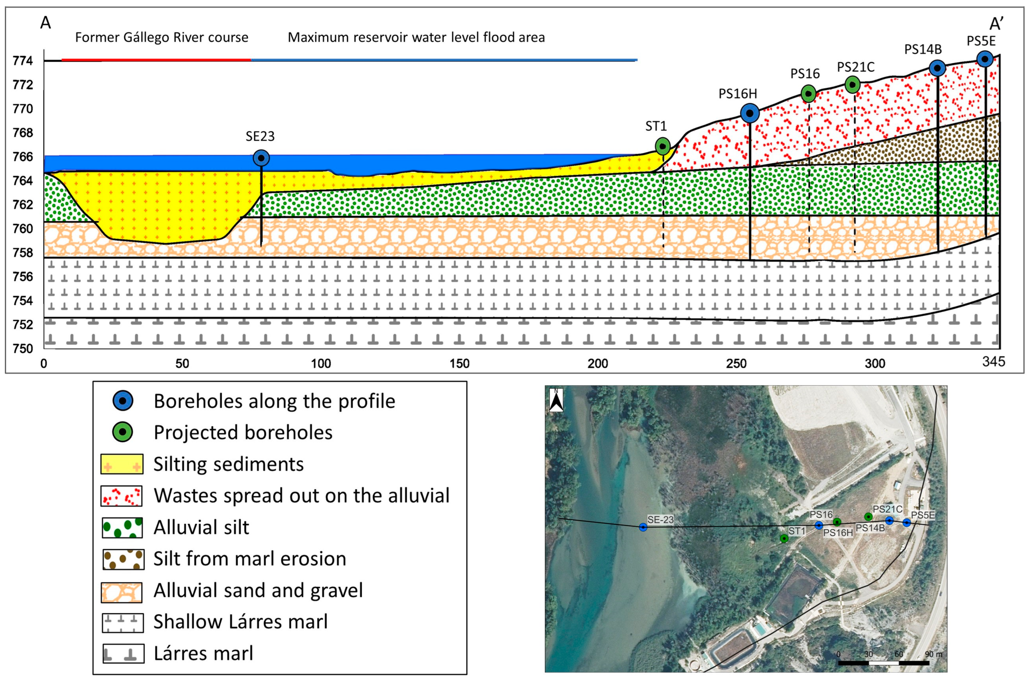
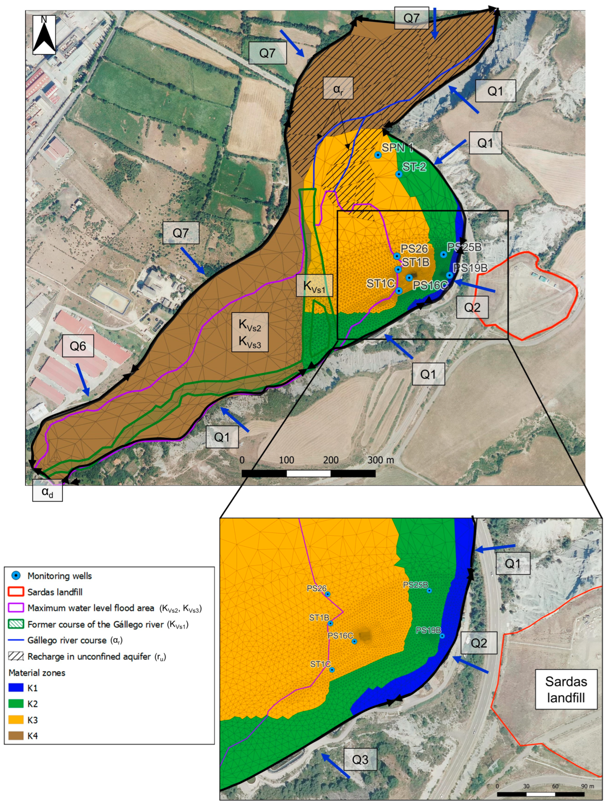

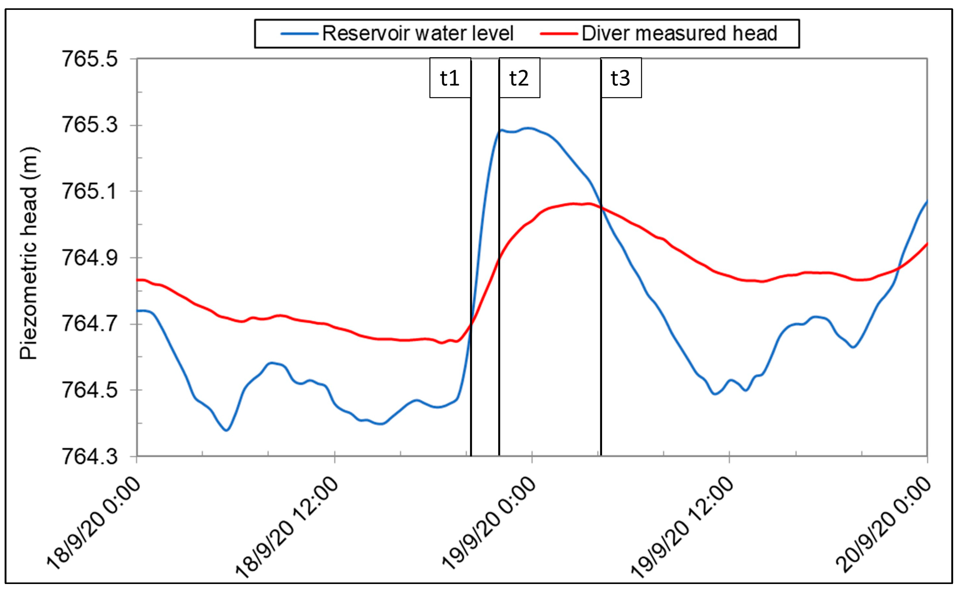
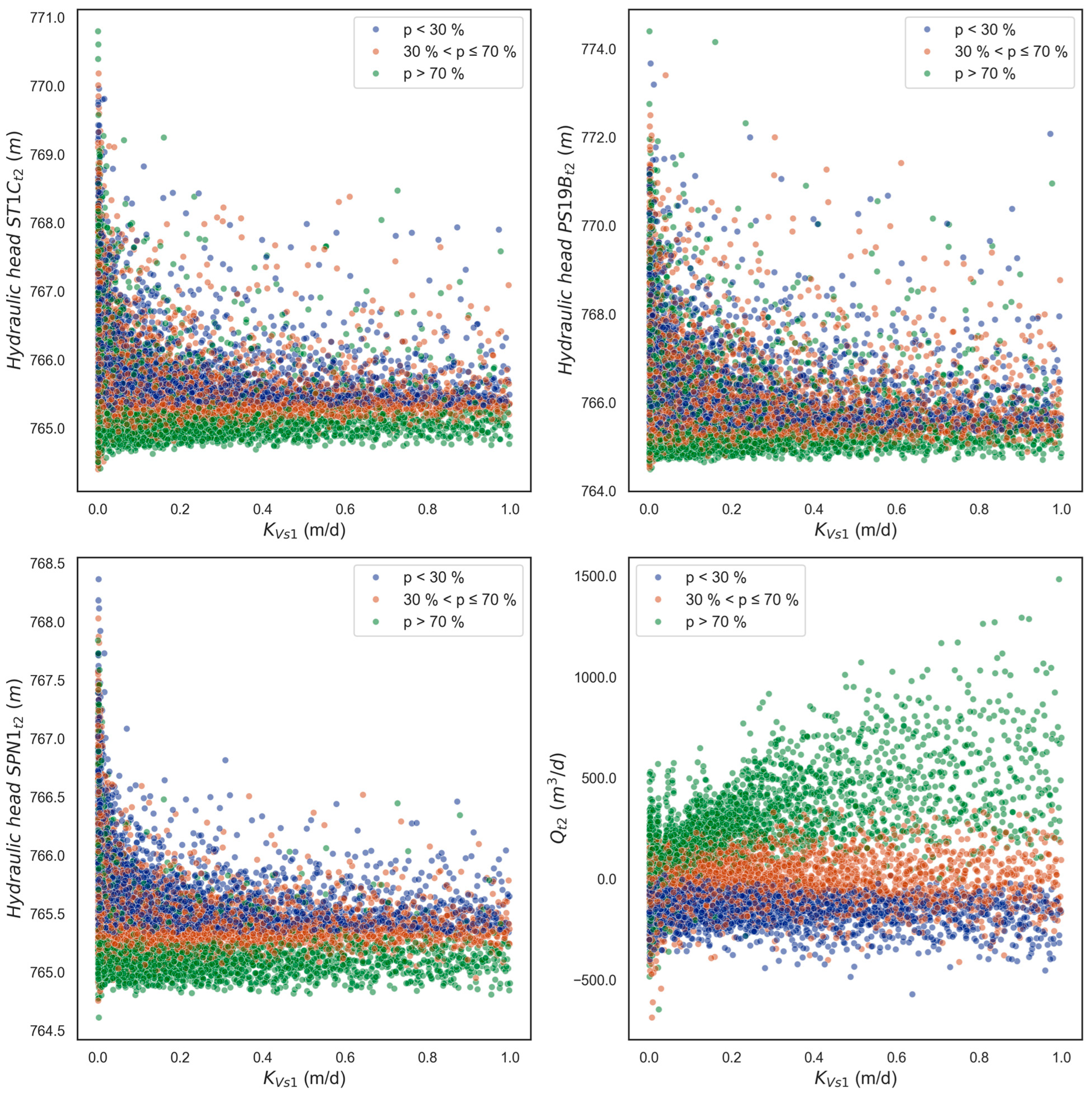
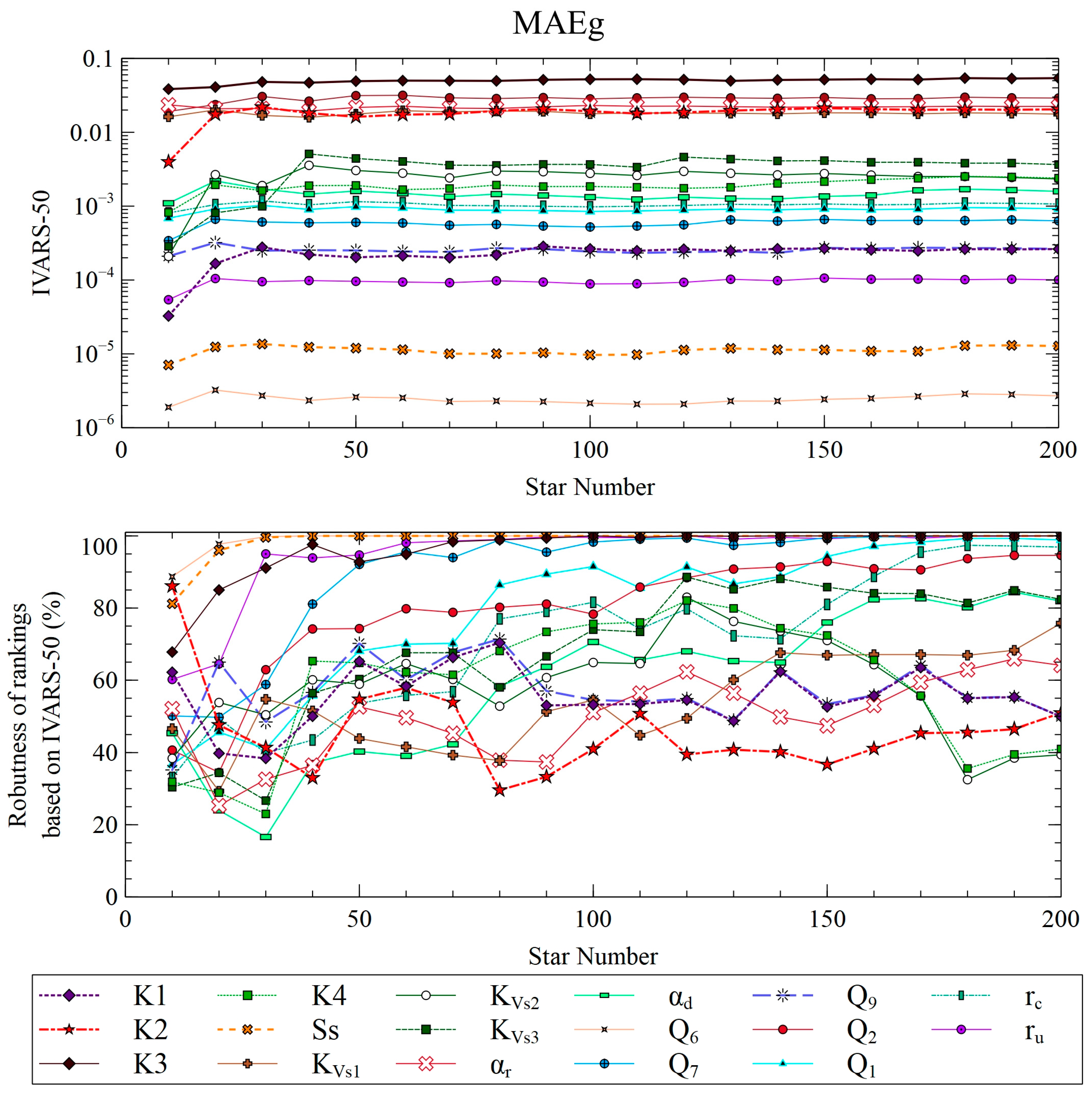
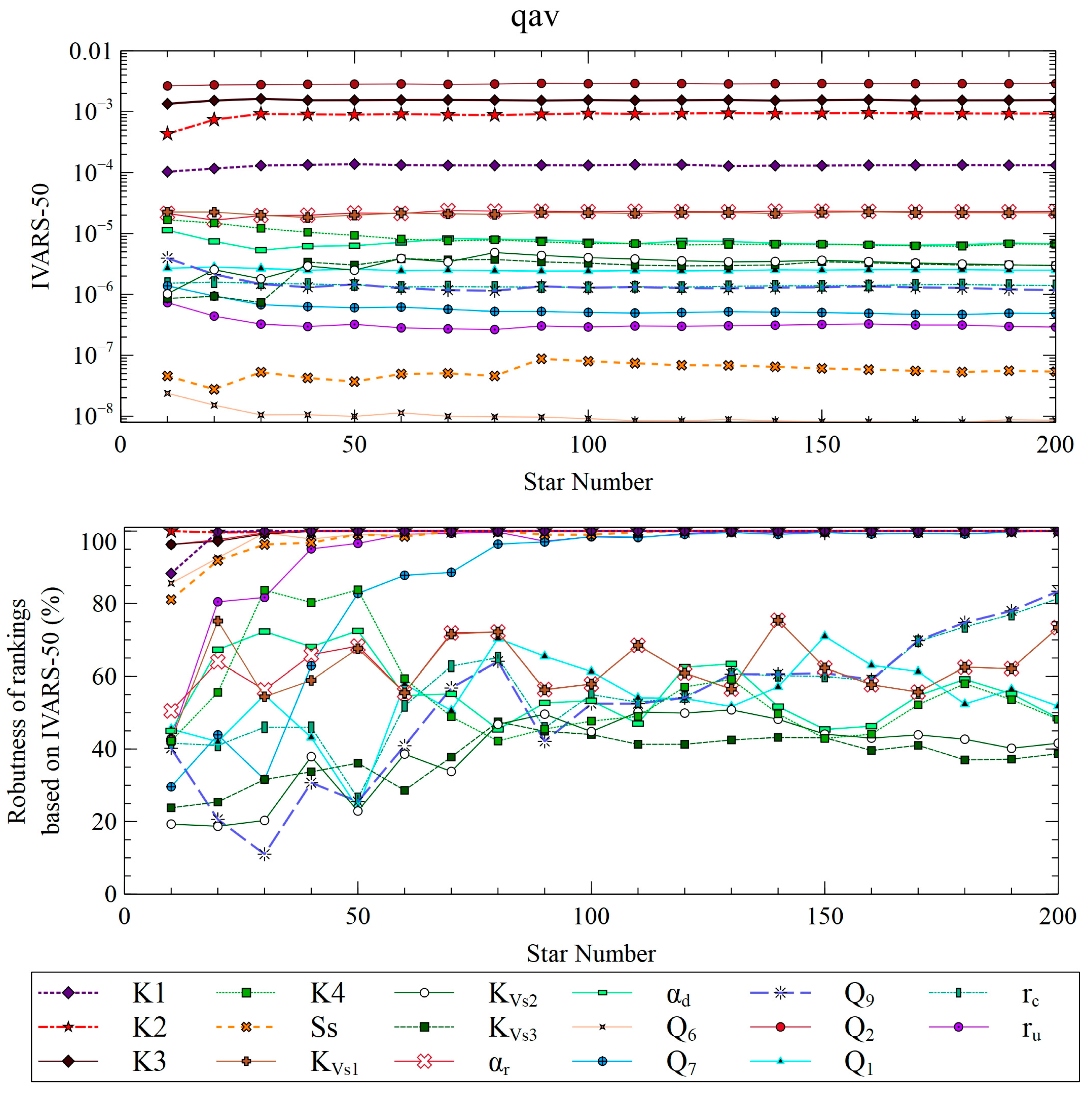
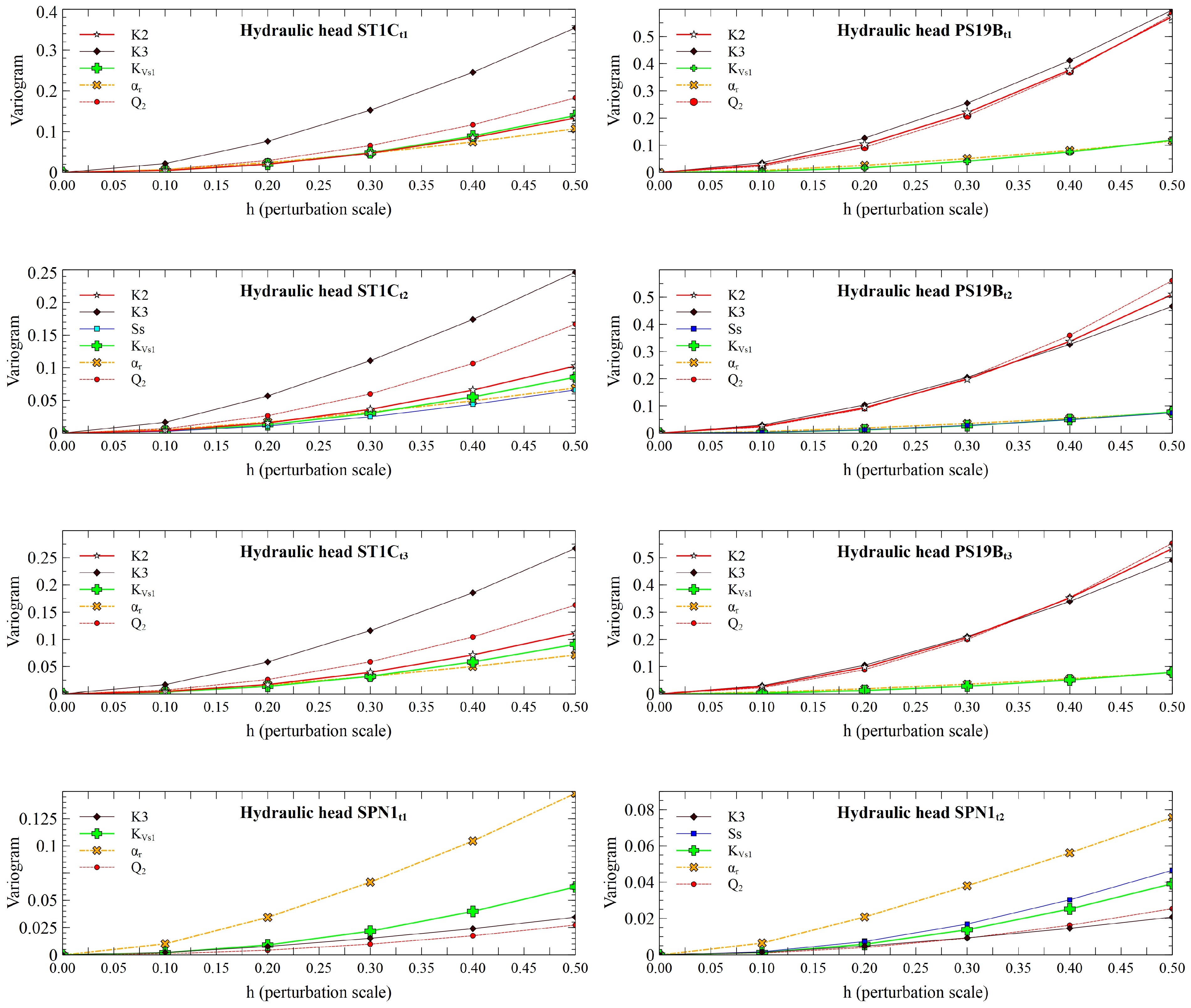
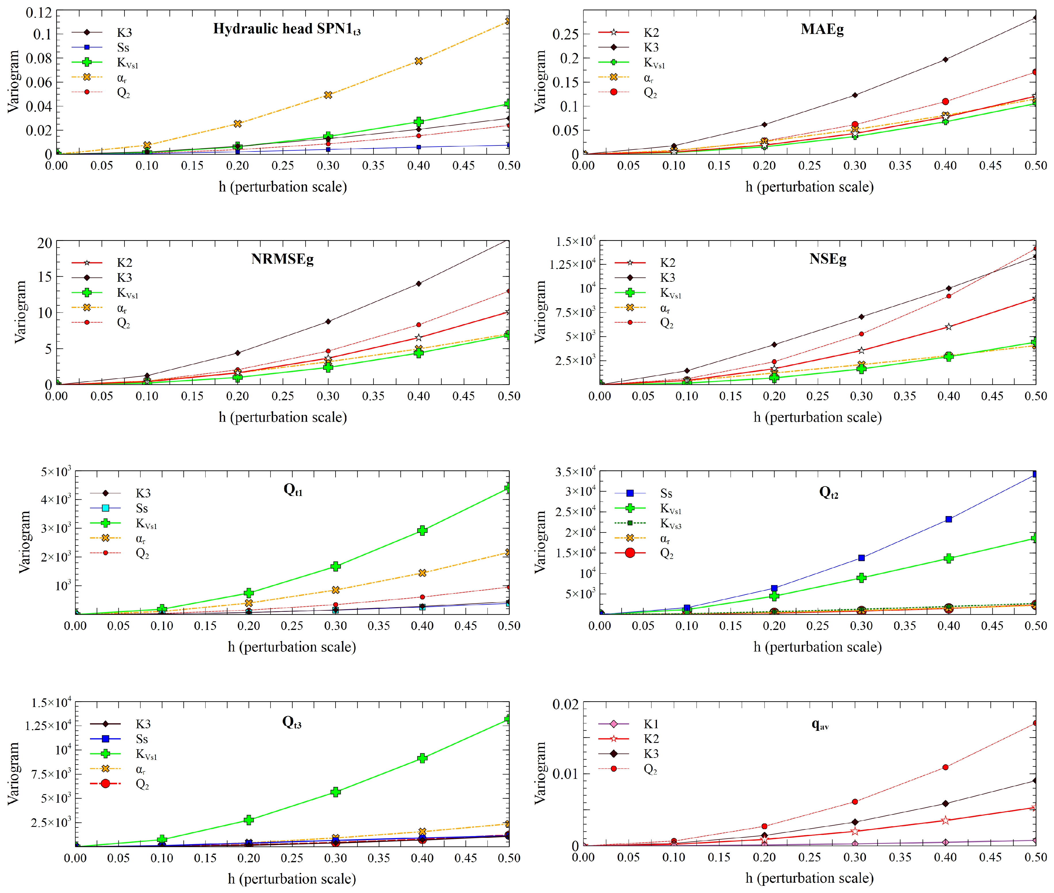
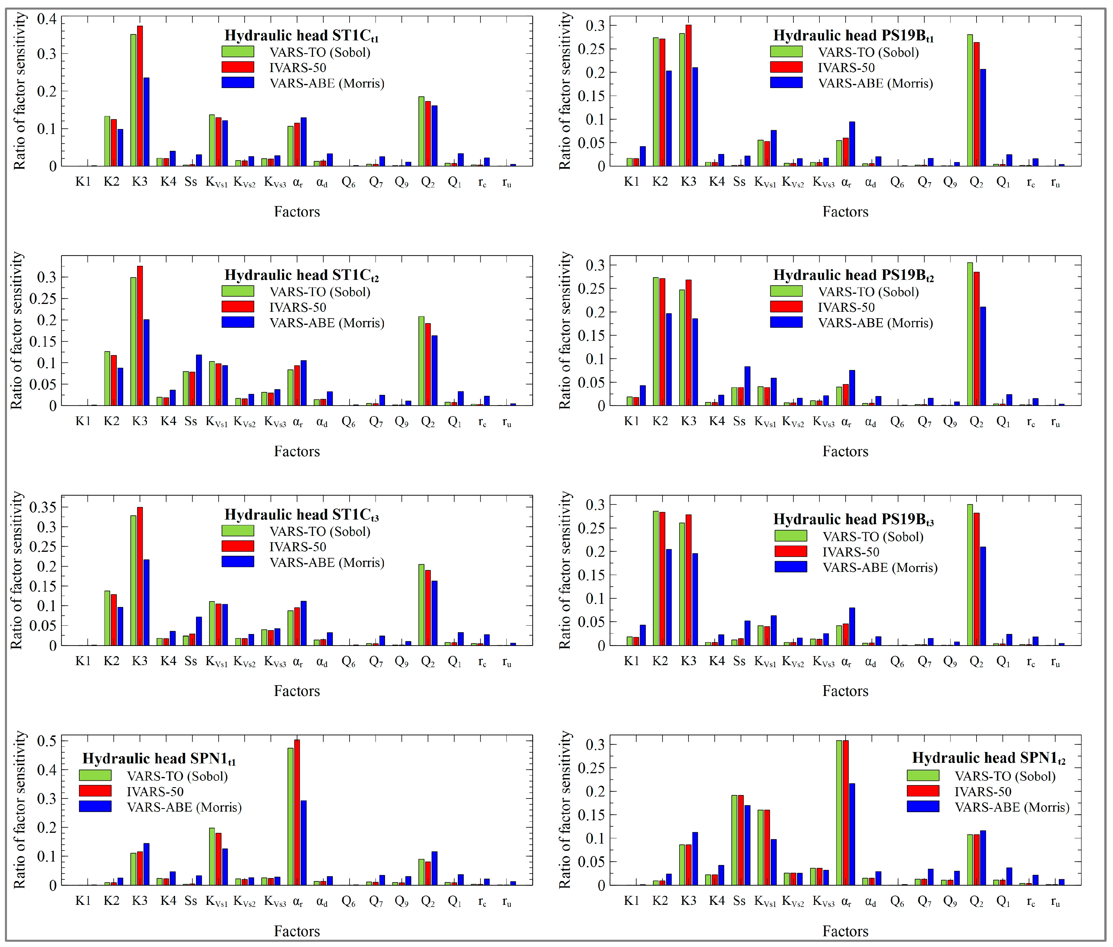
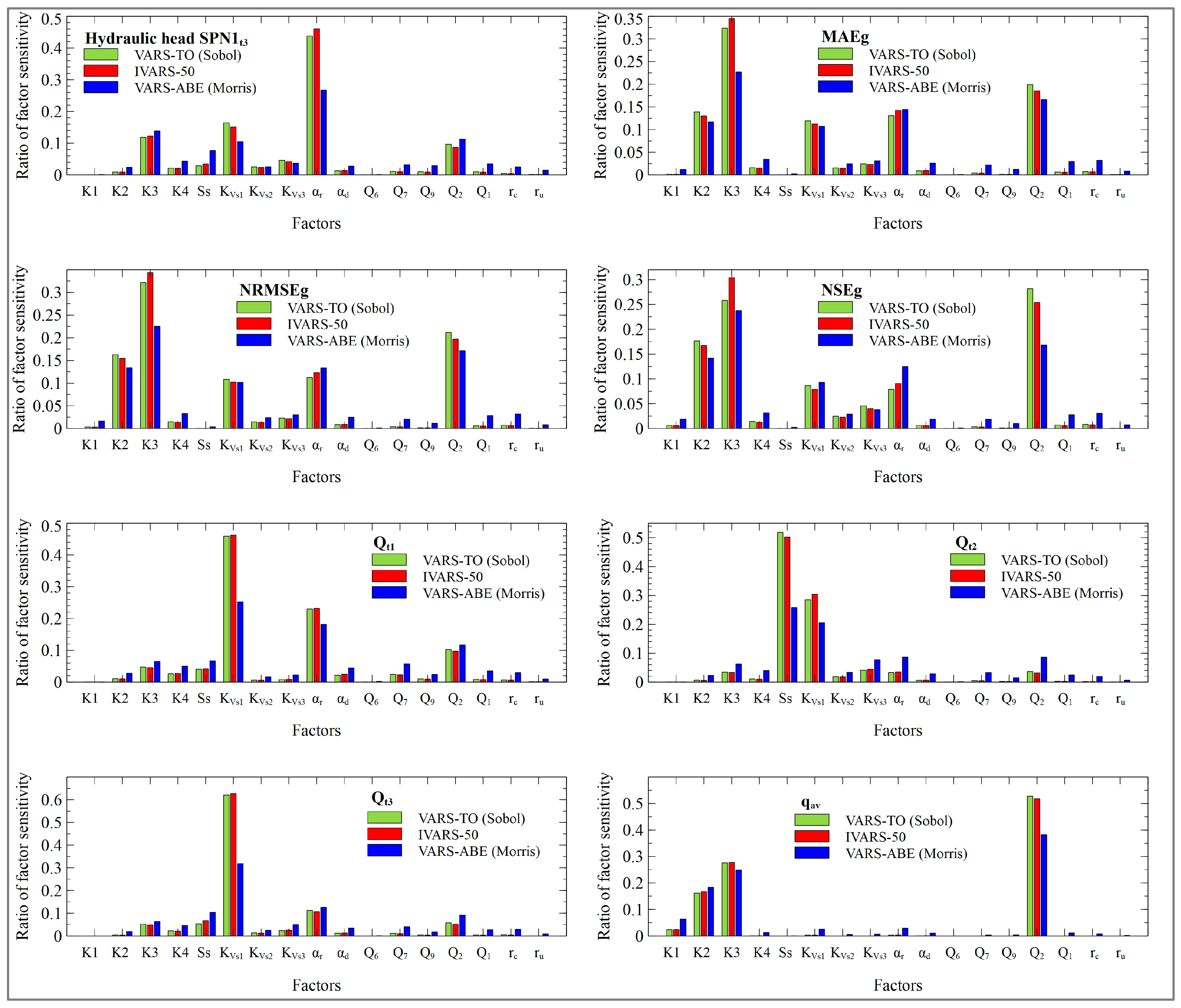
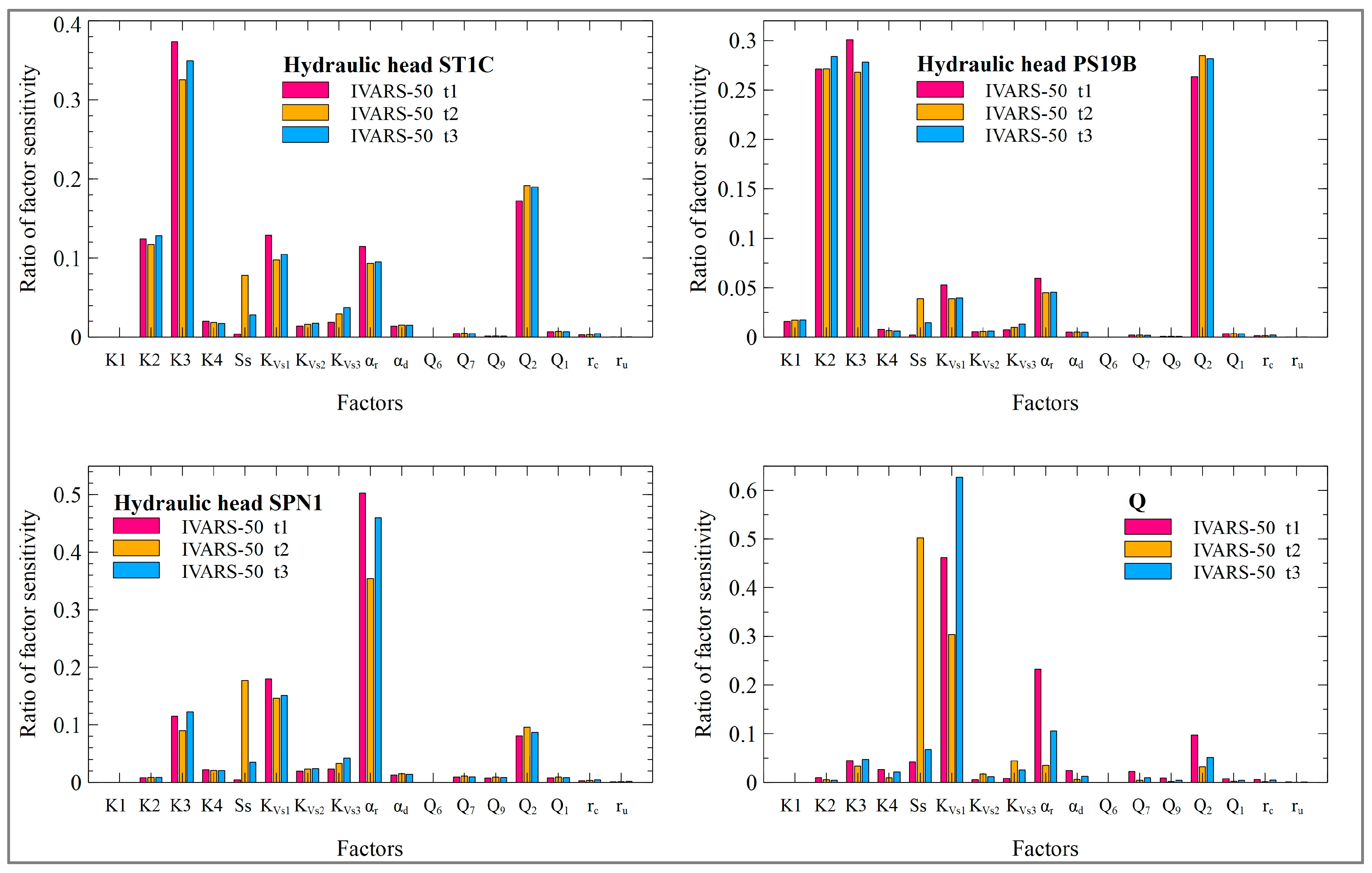
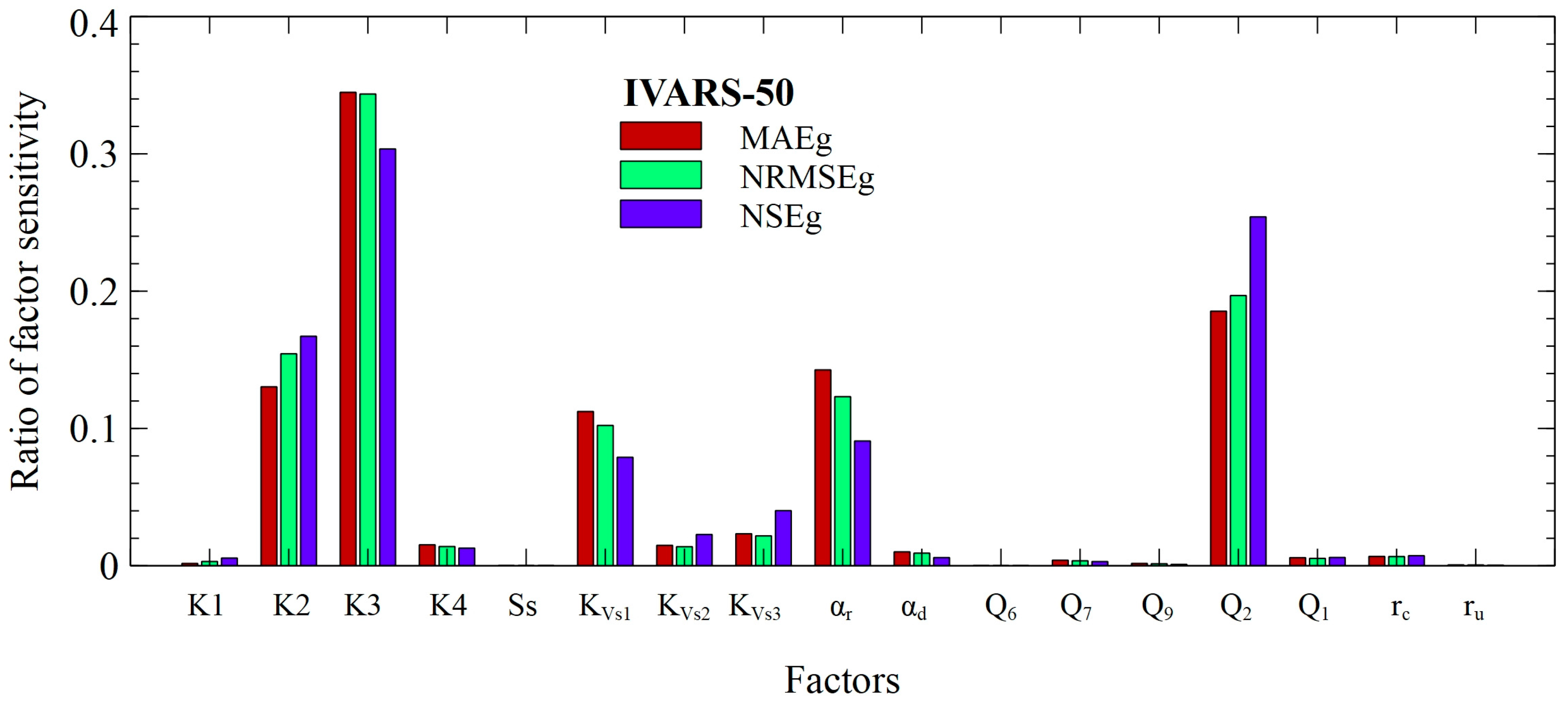
Disclaimer/Publisher’s Note: The statements, opinions and data contained in all publications are solely those of the individual author(s) and contributor(s) and not of MDPI and/or the editor(s). MDPI and/or the editor(s) disclaim responsibility for any injury to people or property resulting from any ideas, methods, instructions or products referred to in the content. |
© 2024 by the authors. Licensee MDPI, Basel, Switzerland. This article is an open access article distributed under the terms and conditions of the Creative Commons Attribution (CC BY) license (https://creativecommons.org/licenses/by/4.0/).