A Quasi-Steady Model for Estimating the Rate of Frost Heave When Subjected to Overburden Pressure

Abstract

The soil beneath buildings constructed in cold regions is affected by frost heave, causing the walls to crack and even the buildings to incline and collapse. Therefore, predicting the frost heave when subjected to overburden pressure is crucial for engineering buildings in cold areas. Utilizing the conservation equation of mass, Darcy’s equation, and the assumption that the pore water pressure at the top of a frozen fringe, denoted as u_w, during the quasi-steady state can be approximately estimated using the Clapeyron equation, a quasi-steady frost heave rate model considering the overburden pressure was proposed. This study considered the difference in pore water pressure within the frozen fringe, which causes water to move from the unfrozen zone to the ice lens, where it subsequently accumulates and freezes into ice. The pore water pressure at the bottom of the frozen fringe, denoted as u_u, can be estimated using the soil water characteristic curve (SWCC). The thickness of the frozen fringe was determined using the freezing temperature, segregation temperature, and temperature gradient. The segregation temperature was determined using the two-point method. Additionally, the model suggested that, when u_w = u_u, the movement of water stopped, leading to the end of frost heave. To validate the proposed model, three existing frost-heaving experiments were analyzed. The findings demonstrated that the estimated rates of frost heave of the samples closely matched the experimental data. Additionally, external pressure delayed water migration. This study can offer theoretical support for building engineering in cold regions.

1. Introduction

The phenomenon of frost heave has caused great damage to constructions in cold regions [1,2,3,4,5,6]. In addition, the construction of taller buildings is bound to be affected by the frost-heaving deformation of the underlying soil. Therefore, it is necessary to develop a model to estimate frost heave when subjected to overburden pressure.

Earlier theories on frost heave suggested that frost heave, which occurs within a closed system without a water supply, is caused by the in situ freezing of soil water into ice, leading to an expansion in volume. Nonetheless, Taber [7,8] discovered in both laboratory and field studies that water movement and the formation of an ice lens also occurred in a closed system. Generally, there are three conditions for frost heave to occur [9]. (1) Soil type: It is known that coarse soils are not susceptible to frost heaving [10]. (2) Availability of water: As soil freezes in a closed system, soil water can be considered as a resource for water migration. (3) Freezing conditions: As the freezing rate is extremely rapid, soil water does not have sufficient time to move and eventually freezes in situ, preventing an ice lens from forming. In contrast, the water can migrate and an ice lens can form when the freezing rate is slower [11].

To address the adverse impact of frost heave on engineering in cold regions, many frost heave models have been proposed. Earlier on, the capillary theory model, which is also known as primary frost theory, was proposed as a means of estimating frost heave [12]. The model considers the surface tension of water menisci in capillaries as the primary force propelling water movement. However, the model evidently underestimates experimental values and fails to explain discontinuous ice lens formation processes. Therefore, the secondary frost heave theory was proposed [13,14]. This theory holds that there is a special area between the unfrozen soil area and the frozen soil area. This special area is defined as the frozen fringe, where ice and water coexist, but there is no frost heaving. The soil water potential gradient and permeability of the frozen fringe are the key parameters for estimating frost heave. Subsequently, O’Neill [15] put forward the rigid ice model, which considers that pore ice is prone to developing on existing ice to form a solid body. Moreover, a break stress was proposed to assess the timing and location of the formation of a new ice lens [15,16,17,18]. Additionally, Konrad [19] proposed a segregation potential theory [19,20,21,22], suggesting that the water migration rate increases linearly with the temperature gradient in a quasi-steady state. The slope of this linear relationship is referred to as the segregation potential. However, the model demonstrated that a representative segregation potential is difficult to determine in the field, as there are many factors that can affect its value even in laboratory settings. The Clapeyron equation was used in the above-mentioned model to calculate the ice and water pressure, and it is only applicable in a quasi-steady state. When the state is unstable, the equation’s validity needs to be further verified. Therefore, it has specific conditions for its applicability, which can limit the availability of models.

The classical Clapeyron equation describes the relationship between the pressure and temperature of a pure water and ice system in an equilibrium state [23].

$$\left({\displaystyle \frac{1}{{\rho }_w}}-{\displaystyle \frac{1}{{\rho }_i}}\right)u=L_f{\displaystyle \frac{T-T_f}{T_f}};u=u_i=u_w$$

(1)

where ρ and u are the density and pressure, respectively; L_f is the latent heat of fusion, T is the system temperature, and T_f is the freezing temperature. The subscripts i and w refer to pore water and pore ice. During the equilibrium state, u_w = u_i. However, for a three-phase porous medium containing soil, water, and ice, there exists a pressure difference between the ice phase and the water phase, u_w ≠ u_i, when the classical Clapeyron equation is not valid. As a result, a more developed Clapeyron equation was proposed [17,18,23,24,25]:

$${\displaystyle \frac{u_w}{{\rho }_w}}-{\displaystyle \frac{u_i}{{\rho }_i}}=L_f\ln {\displaystyle \frac{T+T_{\mathrm{m}}}{T_{\mathrm{m}}}};T_s\le T<T_f$$

(2)

where T_s is the ice segregation temperature and T_m is the freezing temperature of bulk water. The ice segregation temperature refers to the temperature at which soil water freezes and the ice segregation phenomenon occurs under certain conditions. The ice segregation temperature is usually related to factors such as pore size, soil mineral composition, saturation, and overburden pressure. The developed Clapeyron equation was commonly used to analyze ice–water phase transitions in non-equilibrium states [26], which are not reasonable [11].

However, as an equilibrium state cannot be strictly achieved for freezing soil [27], Equation (2) was assumed to be valid in a quasi-steady state [17,18,24,25], where the temperature gradient remains approximately stable. Therefore, a quasi-steady model for estimating the rate of frost heave when subjected to overburden pressure is proposed, as the Clapeyron equation is not valid in the transient state. The model considers that the soil water potential gradient is the primary force propelling water movement. The soil water potential gradient can be determined by the pore water pressure at the top and bottom of the frozen fringe and the thickness of the frozen fringe. The pore water pressure u_w under overburden pressure can be estimated using the Clapeyron equation. However, this equation is not valid at the freezing front, making it unreasonable for calculating the pore water pressure u_u. As illustrated by Equation (2), the Clapeyron equation is valid in the temperature range of T_s ≤ T < T_f. That is, the Clapeyron equation is valid at the top of the frozen fringe (T = T_s), while it is not valid at the bottom of the frozen fringe (T = T_f). If the Clapeyron equation is used to estimate u_u, u_u will remain constant, which is not consistent with the fact that it decreases with the freezing time during the drainage process. Additionally, the temperature gradient above the freezing temperature does not cause moisture migration. Consequently, using the temperature to estimate u_u by means of the Clapeyron equation is unreasonable. Therefore, the pore water pressure u_u cannot be determined using the Clapeyron equation. Hence, this study proposes a new method for estimating u_u using the SWCC based on the phenomenon of drainage in the unfrozen soil area.

In this study, a quasi-steady model is proposed for the prediction of frost heave under overburden pressure by utilizing the conservation equation of mass, Darcy’s equation, and the Clapeyron equation. To demonstrate the model’s applicability, three existing frost-heaving experiments were analyzed. The predicted values were found to be in good agreement with the tested values, indicating the model’s validity. The application of this model requires the soil temperature gradient, the freezing and segregation temperature, the hydraulic conductivity of the frozen fringe, the soil particle size distribution, the saturation water content, the soil freezing characteristic curve (SFCC), and the overburden pressure.

2. Frost Heave Model

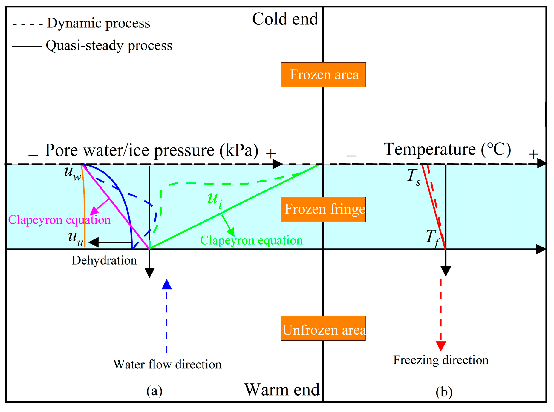
2.1. Physical Model

To present the quasi-steady frost heave model in this study, it was assumed that the Clapeyron equation is applicable at the top of the frozen fringe in the quasi-steady state [25].

Figure 1 illustrates the diagram of the quasi-steady frost heave model. As shown, the model indicates that there is a unique connected region called the frozen fringe situated between the frozen and unfrozen areas. Figure 1a,b illustrate the variations in pore pressure (u_w, u_u, and pore ice pressure u_i) and the temperature of the frozen fringe in both the non-equilibrium state (shown by the dashed line) and the quasi-steady state (shown by the solid line), respectively. The shapes of the curves for pore pressure and temperature in the non-equilibrium state continuously vary as the water content changes. Once the quasi-steady state is achieved, the shape of the curves stabilizes.

As illustrated in Figure 1a, u_w is smaller than u_u in the quasi-steady state, and this difference causes a continuous movement of water from the unfrozen region towards the frozen fringe, where it transforms into ice. The ice formation rate at the top of the frozen fringe is viewed as the frost heave rate. Utilizing the conservation equation of mass, the ice formation rate can be determined using the water flow rate, which largely depends on the soil water potential gradient and the permeability of the frozen fringe. The soil water potential gradient depends on the difference in pore water pressure u_w-u_u and the thickness of the frozen fringe. u_w is mainly controlled by the temperature. In the quasi-steady state, the temperature at the top of the frozen fringe remains relatively stable. Therefore, the Clapeyron equation can be used to determine u_w. The value of u_u calculated with the Clapeyron equation is zero, which is not consistent with real cases. Therefore, this study proposes a new method for estimating u_u.

The proposed model suggests that the unfrozen region in a closed system will experience drainage as water moves continuously toward the frozen fringe. As a result, the unfrozen region will transition to an unsaturated region due to the lack of water supply. Therefore, u_u can be evaluated according to the soil’s unsaturated state, which is indicated by the SWCC. Once the water content at the freezing front is established, the related value of u_u can be obtained using the SWCC. Furthermore, u_u diminishes as the water content at the freezing front decreases during the freezing process. Therefore, the model suggests that water movement will stop as u_u decreases and reaches u_w, leading to the end of frost heave. It is observed that u_w and u_u are negative, whereas the pore ice pressure u_i has a positive value. This is due to the pore ice bearing most of the overburden pressure. u_i is zero at the freezing front, as no ice forms in this position. As the temperature drops, u_i increases due to ice formation. The Clapeyron equation can also be used to assess u_i in the quasi-steady state.

2.2. Derivation of the Mathematical Model

Utilizing the conservation equation of mass, Darcy’s equation, and the assumption that u_w in the quasi-steady state can be approximately estimated using the Clapeyron equation, a mathematical model for the quasi-steady frost heave rate under overburden pressure was derived and presented as follows:

$${\displaystyle \frac{\mathrm{d}h}{\mathrm{d}t}}=-k_f{\displaystyle \frac{{\rho }_w}{{\rho }_i}}{\displaystyle \frac{GradT}{T_s-T_f}}\left\{{\rho }_w{L}_f{\displaystyle \frac{T_s-T_f}{T_m}}+P+{\phi }_e{\left[{\displaystyle \frac{W\left(T_{\mathrm{s}}\right)}{W_s}}\right]}^{-b}-{\phi }_e{\left[{\displaystyle \frac{W\left(T_{\mathrm{f}}\right)}{W_s}}\right]}^{-b}\right\}$$

(3)

where h is the frost heave amount, t is the freezing time, $k_f$ is hydraulic conductivity at the top of frozen fringe, GradT is the temperature gradient, P is the overburden pressure, ${\phi }_e$ is the air entry value of SWCC, $W\left(T\right)$ is the water content at the temperature of T, $W_{\mathrm{s}}$ is the saturation water content, and b is an empirical parameter.

The soil water potential gradient of the frozen fringe is considered to be the main factor propelling water movement. The soil water potential difference is equal to u_w − u_u, where u_w is estimated using the Clapeyron equation, and u_u is estimated using the SWCC. The depth of the frozen fringe is evaluated by utilizing the soil temperature gradient and the freezing and segregation temperatures. The specific derivation process of the mathematical model is detailed in Appendix A.

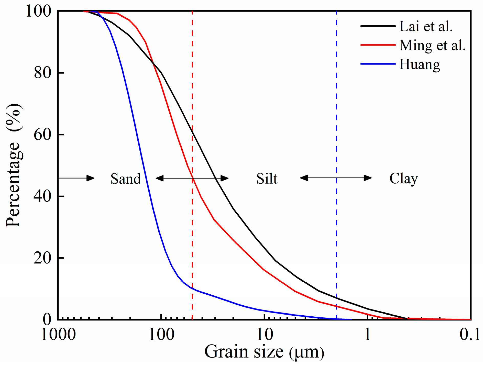
2.3. Soil Sample

To validate the proposed model, three existing frost-heaving experiments that were conducted under external pressures were analyzed in this study. The three soil samples were numbered S1 to S3, and they were reported by Lai et al. [25], Ming et al. [18], and Huang [29], respectively.

Table 1. The physical characteristics of the samples.

Soil Type	W (%)	ρd (g/cm3)	k0 (m/s)	L (cm)	D (cm)
S1 [25]	20.59	1.96	2.15 × 10−8	10	10
S2 [18]	16.17	1.84	2.10 × 10−8	10	10
S3 [29]	35.10	1.49	1.20 × 10−10	11	10

summarizes the properties of the soil samples referenced in the aforementioned studies, where W denotes the initial mass water content, ρ_d indicates the dry density, k₀ represents the saturated unfrozen hydraulic conductivity, and L and D are the samples’ height and diameter.

Table 2. Experimental conditions for the soil samples.

Soil Type	P0 (kPa)	Tc (°C)	Tw (°C)	GradT (°C/cm)
S1 [25]	50, 100	−1.6	1.5	0.31
S2 [18]	0, 100, 200	−2.0	3.0	0.50
S3 [29]	0, 13, 51, 102, 153, 191	−2.0	1.0	0.27

outlines the experimental conditions for the soil samples. P₀ is the overburden pressure, and Tc and Tw are the cold and warm end temperatures. As shown, the three samples were subjected to different overburden pressures and temperature gradients. The temperature gradient imposed on soil sample S3 was the smallest, whereas that applied to soil sample S2 was the largest.

Figure 2 presents the soil particle size distribution curves for the soil samples, which were used to calculate the SWCCs by utilizing Equations (A17) and (A18). The SWCCs were further used to determine the pore water pressure at the bottom of the frozen fringe u_u.

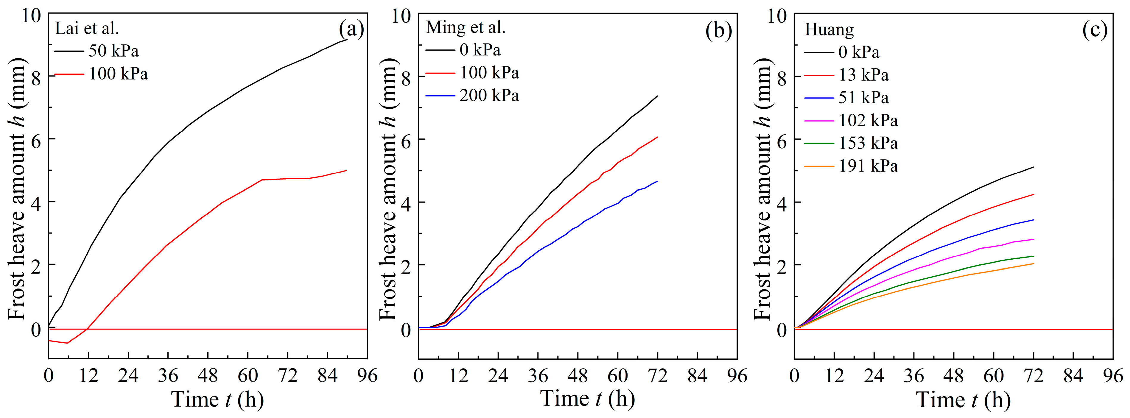
2.4. Frost Heave

Figure 3 illustrates the variations in the amount of frost heave in the aforementioned soil samples in relation to the freezing time under constant pressure. The data indicate that frost heave demonstrated a strong power-law relationship with the freezing time, expressed as follows [9]: $h=a{t}^b+c$. Furthermore, it was observed that frost heave decreased as the overburden pressure increased. This was due to the fact that higher overburden pressure decreased frost heave by postponing water migration [25]. Additionally, it can be observed that the amount of frost heave in the soil samples from Huang [29] was relatively smaller than that in the other two soil samples. This was because the temperature gradient in the soil samples from Huang [29] was the smallest.

3. Results and Discussion

3.1. Parameters of the Model

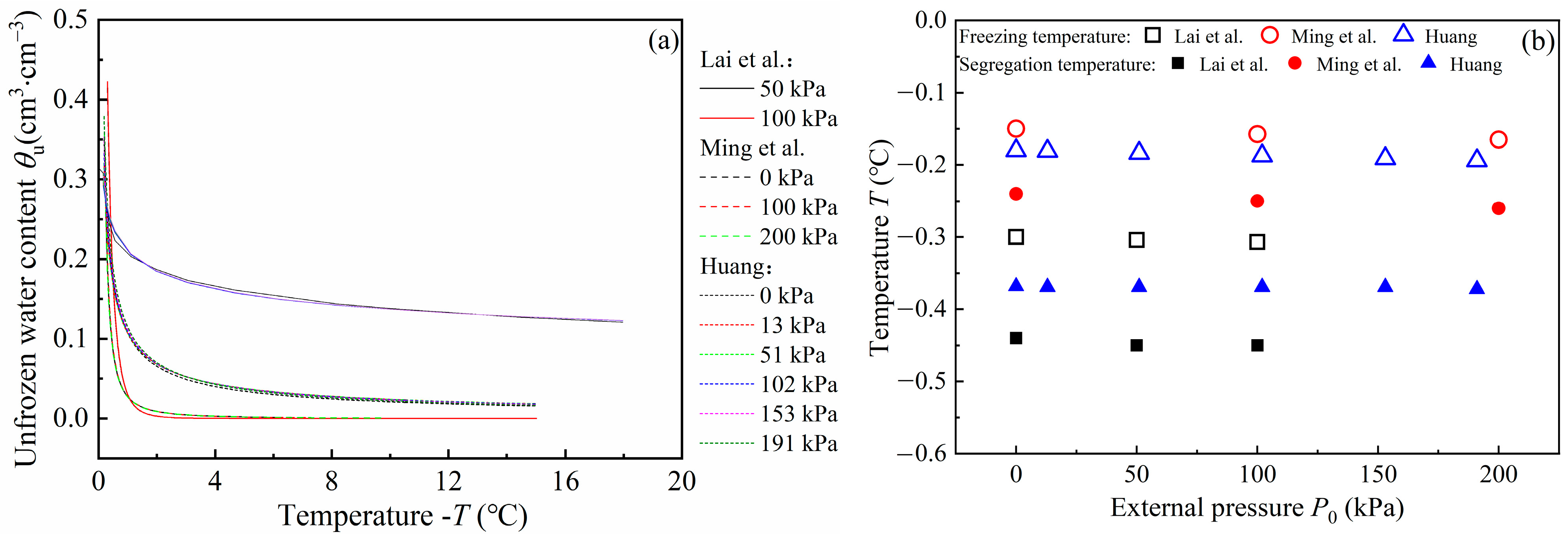
3.1.1. Characteristic Curve of Soil Freezing and the Freezing Temperature under External Pressure

Figure 4a illustrates the SFCCs for the soil samples. As depicted, the unfrozen water content initially rapidly decreased with a decrease in temperature, suddenly slowed down, and remained stable. The unfrozen water content under load was calculated with Equation (A22). Figure 4b illustrates the variations in the freezing and segregation temperatures with the overburden pressure. The freezing temperatures under different external pressures were estimated using Equation (A21), while the segregation temperatures under different external pressures were estimated using the two-point method by means of the soil freezing curves at various external pressures [9]. The results indicate that both the freezing and segregation temperatures slightly decreased with the increase in external pressure, which was likely due to the relatively low level of pressure applied. This effect can be attributed to the fact that the external pressure restricted the soil water, leading to a reduction in kinetic energy.

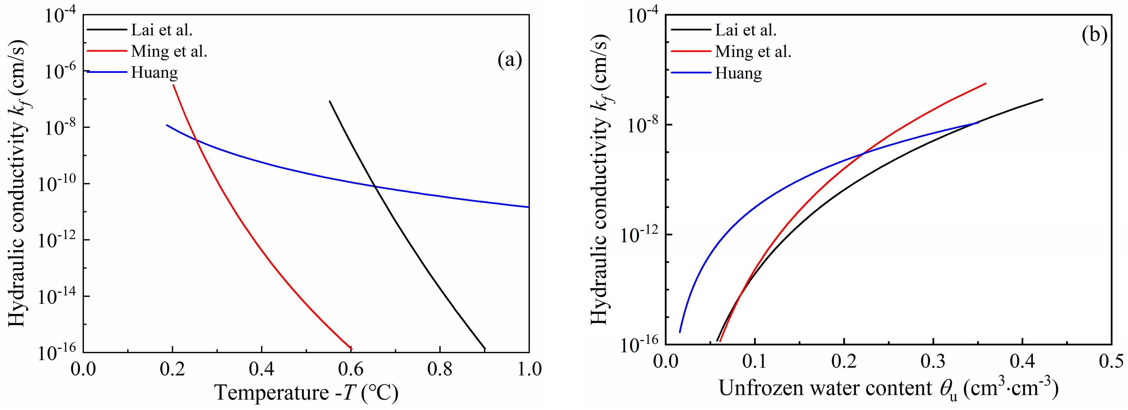
3.1.2. Pore Water Pressure and Hydraulic Conductivity at the Top of the Frozen Fringe

Figure 5a illustrates how u_w changed in response to the overburden pressure, as calculated using Equation (A16). As shown, u_w was negative. This occurred because the temperature dropped from the freezing front to the top of the frozen fringe, leading to a reduction in unfrozen water at the top of the frozen fringe. This led to the formation of the suction, which was due to negative pore water pressure. Additionally, u_w increased as the overburden pressure increased. The reason was that the overburden pressure decreased the ice segregation temperature, resulting in a reduction in u_w with the overburden pressure.

Figure 5b presents the SWCC of the soil sample from Huang [29], which was determined using Equations (A17) and (A18). u_u could be obtained using the SWCC and the water content at this location after tests. As shown, the matric potential decreased with the decrease in water content. This can be explained by the fact that a decrease in water content led to an increase in pore air pressure, which, in turn, raised the matric suction. The matric potential values of the other two soil samples were zero, as the freezing experiments were conducted in a water supply system.

Figure 6 illustrates the relationships between the hydraulic conductivity of the soil samples and both the temperature and unfrozen water content, which were calculated using Equation (A23). As shown, the hydraulic conductivity of the soil samples exponentially decreased as the temperature and unfrozen water content decreased. This occurred because the soil pores filled with unfrozen water acted as pathways for seepage; as the temperature decreased, these pores could freeze, obstructing the seepage channels and leading to a reduction in hydraulic conductivity.

Table 3. Parameters of the soil particle size distribution.

Soil Type	${\mathit{m}}_{\mathbf{cl}}\left(\mathit{\%}\right)$	${\mathit{m}}_{\mathbf{si}}\left(\mathit{\%}\right)$	${\mathit{m}}_{\mathbf{sa}}\left(\mathit{\%}\right)$	${\mathit{d}}_{\mathit{g}}\left(\mathbf{mm}\right)$	${\mathit{\sigma }}_{\mathit{g}}$	$2\mathit{b}+2$
Silty clay [29]	0.28	89.8	9.92	0.70	3.16	5.66
Silty clay [25]	7.03	54.11	38.86	0.09	8.45	12.19
Silty clay [18]	4.38	41.39	54.23	0.17	8.08	10.15

presents the parameters for soil particle size distribution, which were derived from Figure 2; they were utilized to determine ${\phi }_e$ and the hydraulic conductivity of the frozen fringe. m_cl, m_si, and m_sa are the clay, silt, and clay content, respectively. $d_g$ is the geometric mean particle size, and ${\sigma }_g$ is the geometric standard deviation.

3.2. Model Verification

Figure 7a depicts the correlation between the final frost heave rate and the overburden pressure for the three soil samples. It was evident that as the overburden pressure increased, there was a significant decrease in the final frost heave rate. This clearly indicated that the external pressure had a noticeable impact on the frost heave of the soil, as previously discussed. In Figure 7b, scatterplots comparing the predicted frost heave rate with the measured rates for the three soil samples are presented, demonstrating the proposed model’s capabilities. As shown, the solid black line stands for the situation where the predictions match the measured values. The data points were generally close to the solid line, which indicated that the proposed model accurately fit the measured data. However, only one data point for Ming [18] at 200 kPa was somewhat further from the solid line. Overall, the proposed model demonstrated a good ability to predict frost heave.

To further investigate the proposed model, an error range for the frost heave rate was established by utilizing the acceptable experimental error range of hydraulic conductivity [30], as presented in Figure 7b. It can be observed that all of the scatters except one fell within the error range, suggesting that the current model is reliable. Additionally, the model performance was further demonstrated by the mean difference and the root mean square error, which are expressed as

$$\mathrm{MD}={\displaystyle \frac{{\displaystyle \sum _{i=1}^N\left(\ln h_p-\ln h_t\right)}}{N}}$$

(4)

$$\mathrm{RMSE}=\sqrt{{\displaystyle \frac{{\displaystyle \sum _{i=1}^N{\left(\ln h_p-\ln h_t\right)}^2}}{N}}}$$

(5)

where h_p is the predicted frost heave amount, and h_t is the measured frost heave amount. As the data for frost heave rates were extremely small, it was necessary to log-transform them to ensure that the complete range of frost heave rates was well represented. The MD and RMSE values for the silty clay from Huang [29] were 0.19 and 0.55, respectively, those for the sample from Lai et al. [25] were 0.476 and 0.227, respectively, and those for the sample from Ming et al. [18] were −0.123 and 2.94, respectively. The lower RMSE values suggested that the proposed model effectively captured the changes in the frost heave rate in response to overburden pressures.

4. Conclusions

This study proposed a quasi-steady model for frost heave rates influenced by overburden pressures by utilizing the mass conservation law, Darcy’s law, and the assumption that the pore water pressure at the top of frozen fringe u_w can be estimated using the Clapeyron equation when in the quasi-steady state. The model suggested that the frost heave rate when subjected to overburden pressure is primarily governed by that pressure. The model’s performance was evaluated using test results. The key conclusions are as follows.

(1)

The proposed model suggested that the soil water potential gradient of the frozen fringe is the primary force propelling water movement. The difference in soil water potential is defined as u_w-u_u, where u_w can be calculated using the Clapeyron equation, and u_u can be determined with the soil water characteristic curve. Additionally, the model suggested that, when u_w = u_u, the water movement stops, leading to the end of frost heave.

(2)

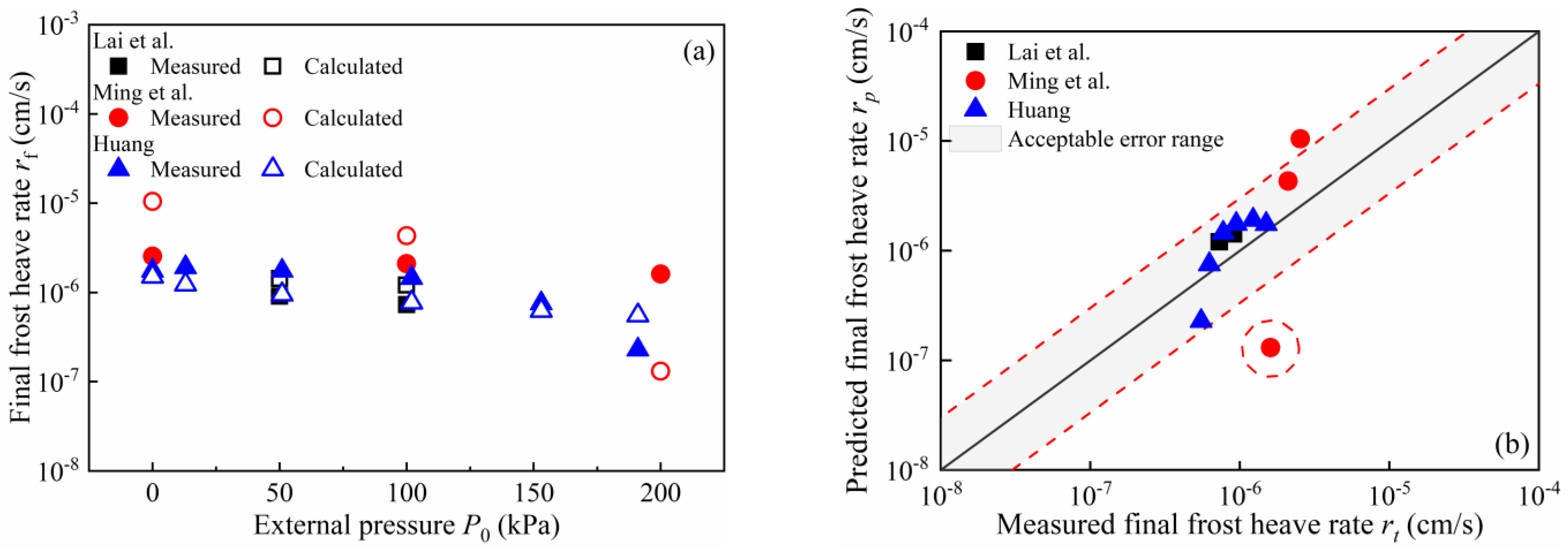
To assess and examine the proposed model, three existing frost-heaving experiments were studied. The findings revealed that the predicted frost heave rates for the soil samples closely matched the experimental data overall, demonstrating the model’s validity.

(3)

The model is easy to apply as long as the SFCC, the soil particle size distribution, the overburden, the freezing point, the saturated hydraulic conductivity, and the saturation water content are provided.

References

- Yang, Z.H.; Dutta, U.; Xiong, F.; Biswas, N.; Benz, H. Seasonal frost effects on the dynamic behavior of a twenty-story office building. Cold Reg. Sci. Technol. 2008, 51, 76–84. [Google Scholar] [CrossRef]
- Wang, Y.P.; Jin, H.J.; Li, G.Y. Investigation of the freeze–thaw states of foundation soils in permafrost areas along the China–Russia Crude Oil Pipeline (CRCOP) route using ground-penetrating radar (GPR). Cold Reg. Sci. Technol. 2016, 126, 10–21. [Google Scholar] [CrossRef]
- Kanie, S.; Akagawa, S.; Kim, K.; Mikami, T. Estimation method of frost heaving for chilled gas pipeline buried in frost susceptible soil. Cold Reg. Eng. 2006, 20, 1–12. [Google Scholar] [CrossRef]
- Kraatz, S.; Jacobs, J.M.; Miller, H.J. Spatial and temporal freeze-thaw variations in Alaskan roads. Cold Reg. Sci. Technol. 2019, 157, 149–162. [Google Scholar] [CrossRef]
- Wu, X.Y.; Niu, F.J.; Lin, Z.J.; Luo, J.; Zheng, H.; Shao, Z.J. Delamination frost heave in embankment of high speed railway in high altitude and seasonal frozen region. Cold Reg. Sci. Technol. 2018, 153, 25–32. [Google Scholar] [CrossRef]
- Qin, Z.P.; Lai, Y.M.; Tian, Y.; Yu, F. Frost-heaving mechanical model for concrete face slabs of earthen dams in cold regions. Cold Reg. Sci. Technol. 2019, 161, 91–98. [Google Scholar] [CrossRef]
- Taber, S. Frost heaving. J. Geol. 1929, 37, 428–461. [Google Scholar] [CrossRef]
- Taber, S. The mechanics of frost heaving. J. Geol. 1930, 38, 303–317. [Google Scholar] [CrossRef]
- Xu, X.Z.; Wang, J.C.; Zhang, L.X. Frozen Soil Physics; Science Press: Beijing, China, 2010. [Google Scholar]
- She, W.; Wei, L.S.; Zhao, G.T.; Yang, G.T. New insights into the frost heave behavior of coarse grained soils for high-speed railway roadbed: Clustering effect of fines. Cold Reg. Sci. Technol. 2019, 167, 102863. [Google Scholar] [CrossRef]
- Bronfenbrener, L.; Bronfenbrener, R. Modeling frost heave in freezing soils. Cold Reg. Sci. Technol. 2010, 61, 43–64. [Google Scholar] [CrossRef]
- Everett, D.H. The thermodynamics of frost damage to porous solids. Trans. Faraday Soc. 1961, 57, 1541–1551. [Google Scholar] [CrossRef]
- Gilpin, R.R. A model for the prediction of ice lensing and frost heave in soils. Water Resour. Res. 1980, 16, 918–930. [Google Scholar] [CrossRef]
- Nixon, J.F. Discrete ice lens theory for frost heave in soils. Can. Geotech. J. 1991, 28, 843–859. [Google Scholar] [CrossRef]
- O’Neill, K.; Miller, R.D. Exploration of a rigid ice model of frost heave. Water Resour. Res. 1985, 21, 281–296. [Google Scholar] [CrossRef]
- Nixon, J.F. Discrete ice lens theory for frost heave beneath pipelines. Can. Geotech. J. 1992, 29, 487–497. [Google Scholar] [CrossRef]
- Zhou, J.Z.; Li, D.Q. Numerical analysis of coupled water, heat and stress in saturated freezing soil. Cold Reg. Sci. Technol. 2012, 72, 43–49. [Google Scholar] [CrossRef]
- Ming, F.; Zhang, Y.; Li, D.Q. Experimental and theoretical investigations into the formation of ice lenses in deformable porous media. Geosci. J. 2016, 20, 667–679. [Google Scholar] [CrossRef]
- Konrad, J.M.; Morgenstern, N.R. The segregation potential of a freezing soil. Can. Geotech. J. 1981, 18, 482–491. [Google Scholar] [CrossRef]
- Konrad, J.M.; Shen, M. 2-D frost heave action model using segregation potential of soils. Cold Reg. Sci. Technol. 1996, 24, 263–278. [Google Scholar] [CrossRef]
- Konrad, J.M. Estimation of the segregation potential of fine-grained soils using the frost heave response of two reference soils. Can. Geotech. J. 2005, 42, 38–50. [Google Scholar] [CrossRef]
- Nixon, J.F. Field frost heave predictions using the segregation potential concept. Can. Geotech. J. 1982, 19, 526–529. [Google Scholar] [CrossRef]
- Ma, W.; Zhang, L.; Yang, C. Discussion of the applicability of the generalized Clausius–Clapeyron equation and the frozen fringe process. Earth-Sci. Rev. 2015, 142, 47–59. [Google Scholar] [CrossRef]
- Kurylyk, B.L.; Watanabe, K. The mathematical representation of freezing and thawing processes in variablysaturated, non-deformable soils. Adv. Water Resour. 2013, 60, 160–177. [Google Scholar] [CrossRef]
- Lai, Y.M.; Pei, W.S.; Zhang, M.Y.; Zhou, J.Z. Study on theory model of hydro-thermal–mechanical interaction process in saturated freezing silty soil. Int. J. Heat Mass Transf. 2014, 78, 805–819. [Google Scholar] [CrossRef]
- Edlefsen, N.E.; Anderson, A.B.C. Thermodynamics of soil moisture. Hilgardia 1943, 12, 117–123. [Google Scholar] [CrossRef]
- Ming, F.; Li, D.Q. A model of migration potential for moisture migration during soil freezing. Cold Reg. Sci. Technol. 2016, 124, 87–94. [Google Scholar] [CrossRef]
- Zhang, X.Y.; Sheng, Y.; Huang, L.; Huang, X.B.; He, B.B. Application of the segregation potential model to freezing soil in a closed system. Water 2020, 12, 2418. [Google Scholar] [CrossRef]
- Huang, L. Study on Mechanical Characteristics in the Process of Interaction between Pipe and Frozen Soil under Frost Heaving Conditions; University of Chinese Academy of Sciences: Lanzhou, China, 2019. [Google Scholar]
- Ming, F.; Chen, L.; Li, D.Q.; Wei, X.B. Estimation of hydraulic conductivity of saturated frozen soil from the soil freezing characteristic curve. Sci. Total Environ. 2020, 698, 134132. [Google Scholar] [CrossRef]
- Ji, Y.; Zhou, G.; Zhao, X.; Wang, J.; Wang, T.; Lai, Z.; Mo, P. On the frost heaving-induced pressure response and its dropping power-law behaviors of freezing soils under various restraints. Cold Reg. Sci. Technol. 2017, 142, 25–33. [Google Scholar] [CrossRef]
- Sheng, D.; Zhang, S.; Niu, F.; Cheng, G. A potential new frost heave mechanism in high-speed railway embankments. Géotechnique 2014, 64, 144–154. [Google Scholar] [CrossRef]
- Lei, Z.D.; Yang, S.X.; Xie, S.C. Soil Hydrodynamics; Tsinghua University Press: Beijing, China, 1988. [Google Scholar]
- Hoekstra, P. Moisture movement in soils under temperature gradients with the cold-side temperature below freezing. Water Resour. Res. 1966, 2, 241–250. [Google Scholar] [CrossRef]
- Mageau, D.W.; Morgenstern, N.R. Observations on moisture migration in frozen soils. Can. Geotech. J. 1980, 17, 54–60. [Google Scholar] [CrossRef]
- Thomas, H.R.; Cleall, P.; Li, Y.C.; Harris, C.; Kern-Luetschg, M. Modelling of cryogenic processes in permafrost and seasonally frozen soils. Géotechnique 2009, 59, 173–184. [Google Scholar] [CrossRef]
- Black, P.B. Application of the Clapeyron Equation to Water and Ice in Porous Media; American Society for Testing and Materials: Philadelphia, PA, USA, 1995. [Google Scholar]
- Henry, K.S. A Review of the Thermodynamics of Frost Heave; Defense Technical Information Center: Fort Belvoir, VA, USA, 2000. [Google Scholar]
- Campbell, G.S. Soil Physics with Basic: Transport Models for Soil-Plant Systems; Elsevier: Amsterdam, The Netherlands, 1985; Volume 14. [Google Scholar]
- Zhou, J.Z.; Wei, C.F.; Lai, Y.M.; Wei, H.Z.; Tian, H.H. Application of the generalized clapeyron equation to freezing point depression and unfrozen water content. Water Resour. Res. 2018, 54, 9412–9431. [Google Scholar] [CrossRef]
- Chen, L.; Zhang, X.Y. A model for predicting the hydraulic conductivity of warm saturated frozen soil. Build. Sci. 2020, 179, 106939. [Google Scholar] [CrossRef]