
Sponge City Drainage System Prediction Based on Artificial Neural Networks: Taking SCRC System as Example

Abstract
1. Introduction
2. Materials and Methods
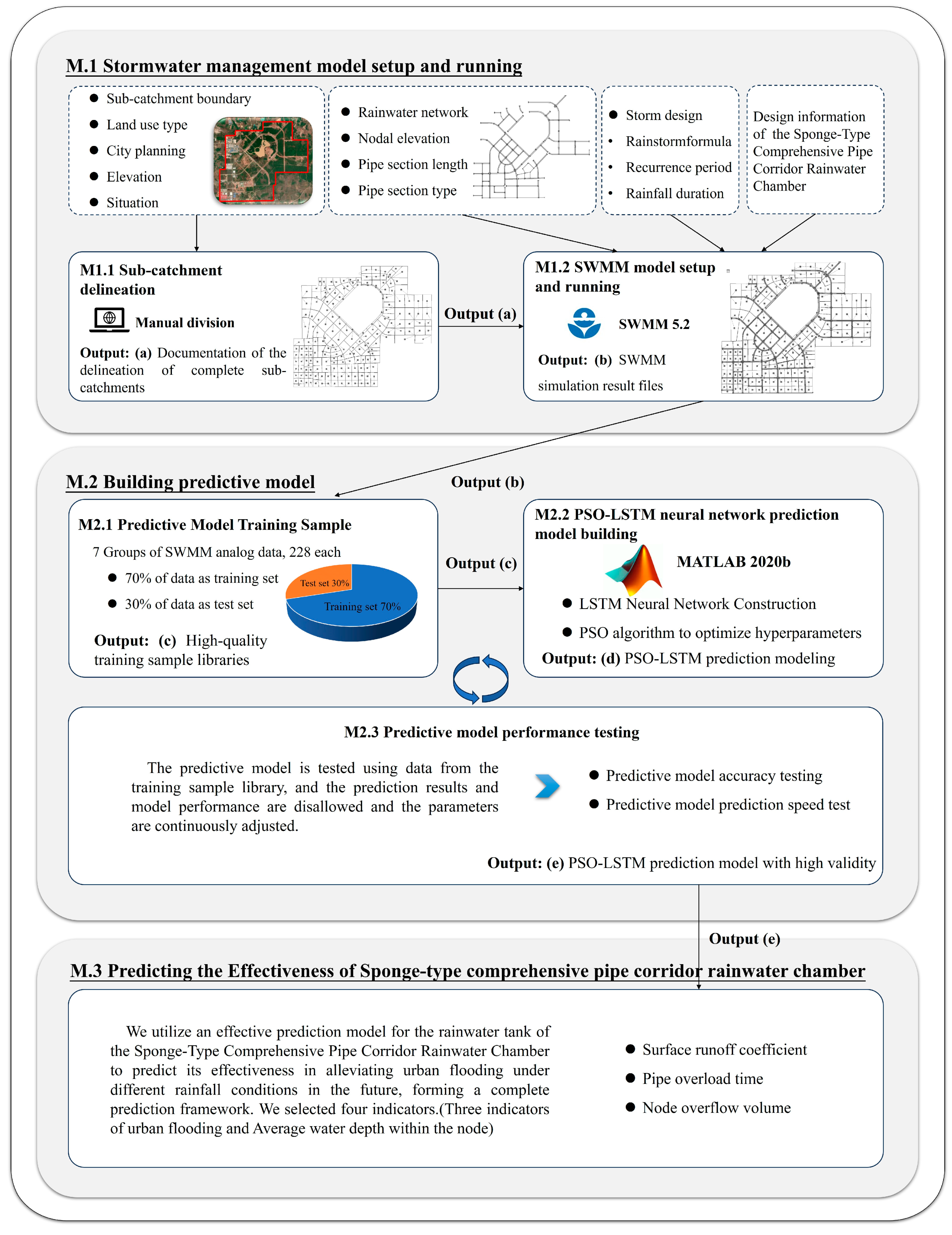
2.1. Research Process
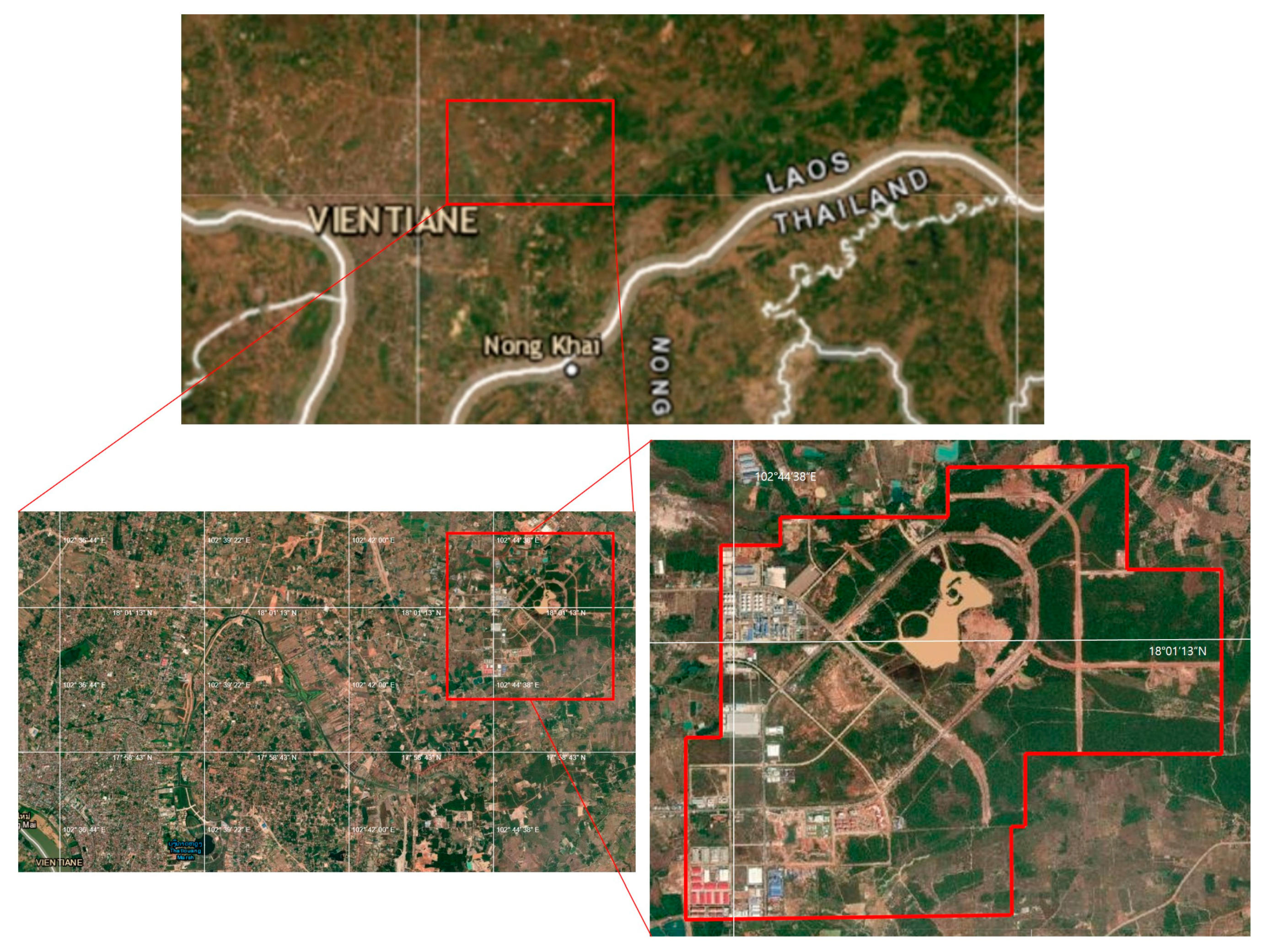
2.2. Study Area
2.3. Storm Water Management Model
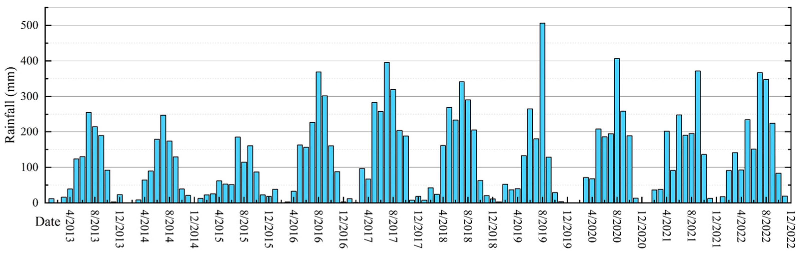
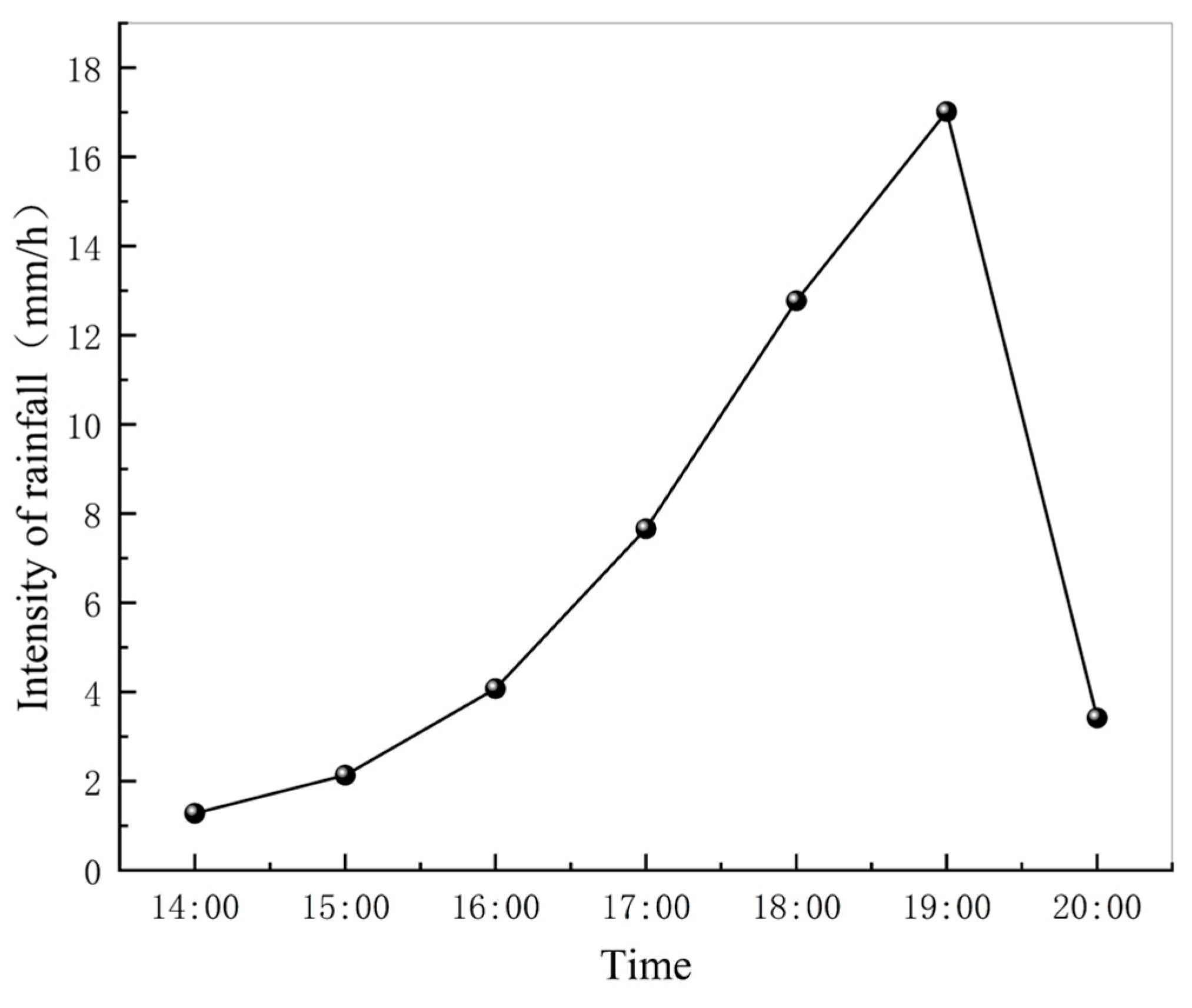
2.3.1. Design Rainfall
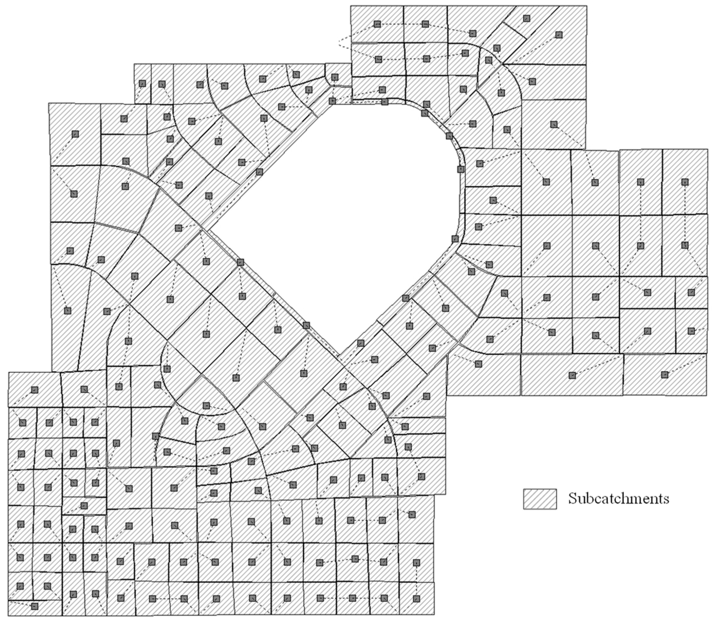
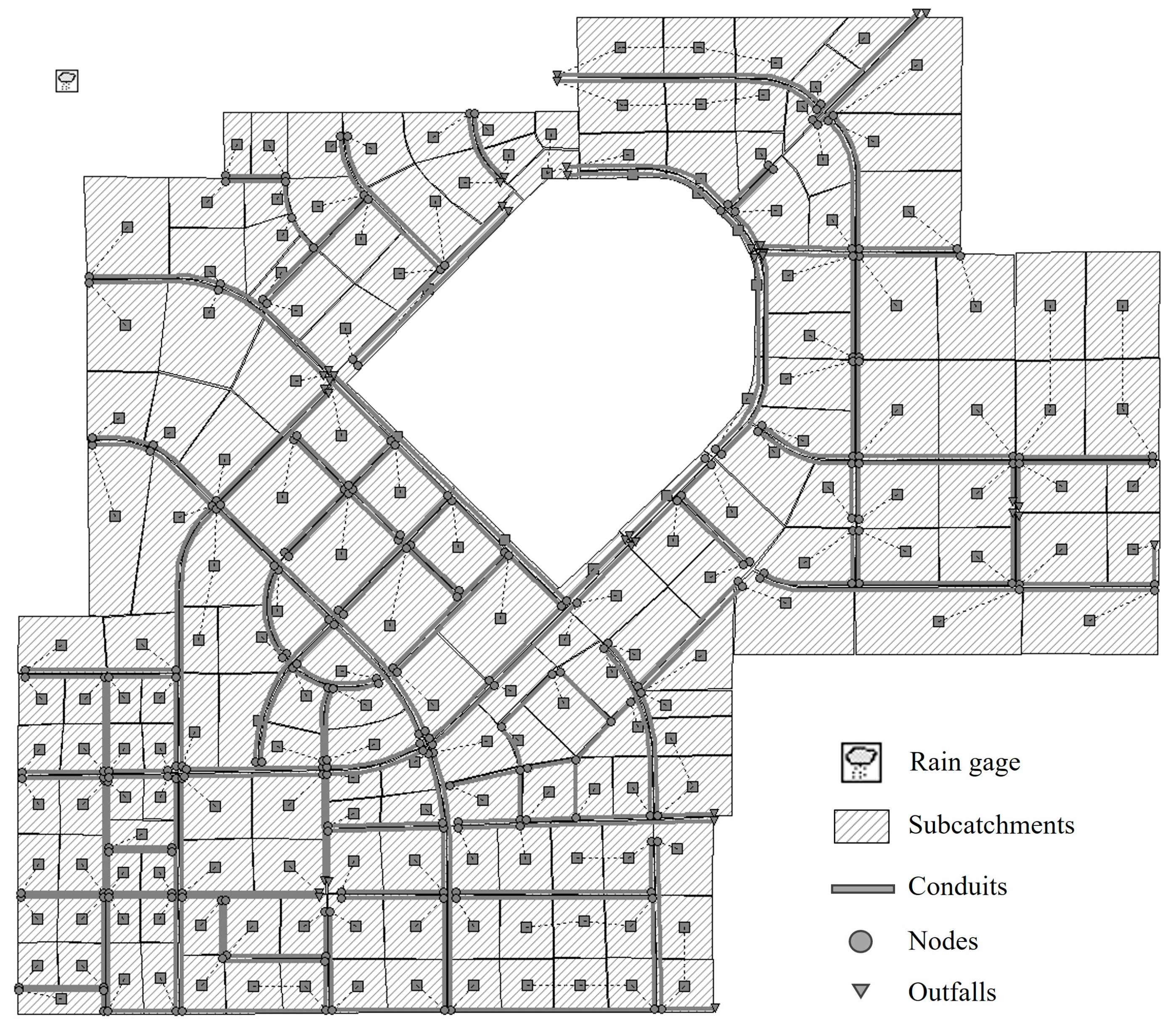
2.3.2. Sub-Catchment Delineation
2.4. The SCRC System Design
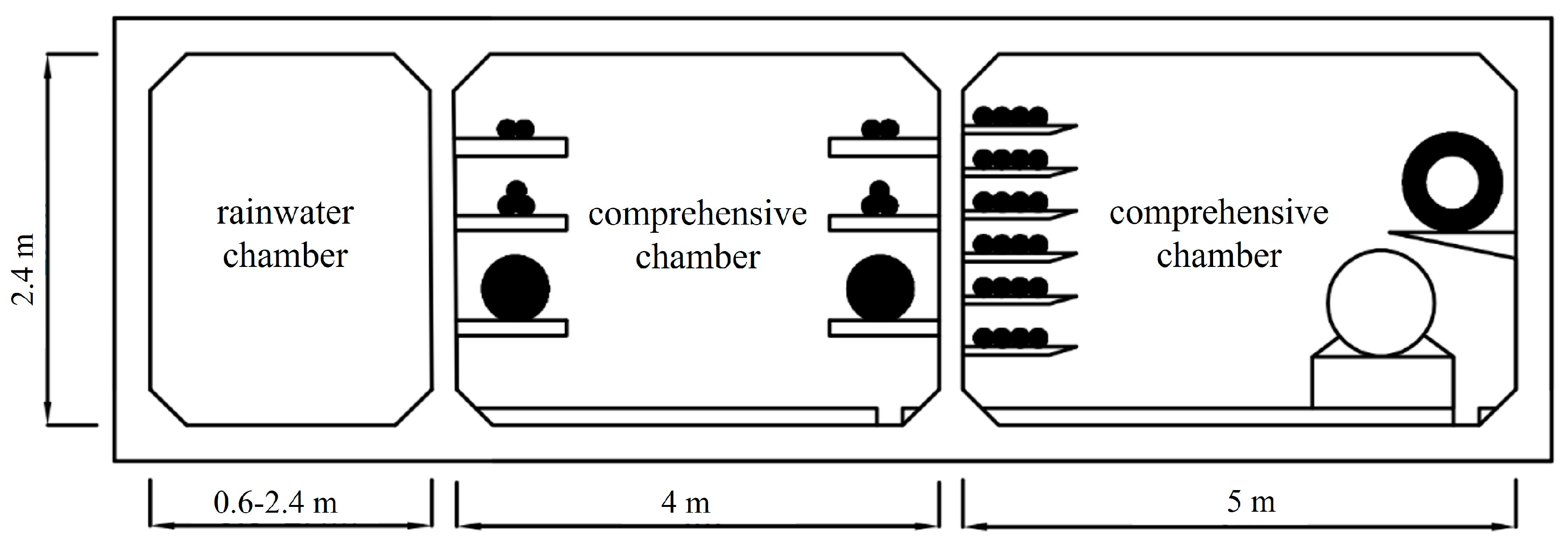
2.4.1. Comprehensive Pipe Corridor Rainwater Chamber
2.4.2. Combination LID Measures
2.4.3. The SCRC System
2.4.4. SWMM Model Building and Running
2.5. Prediction Model
2.5.1. Predictive Model Training Sample
2.5.2. PSO–LSTM Neural Network Prediction Model Building
- (1)
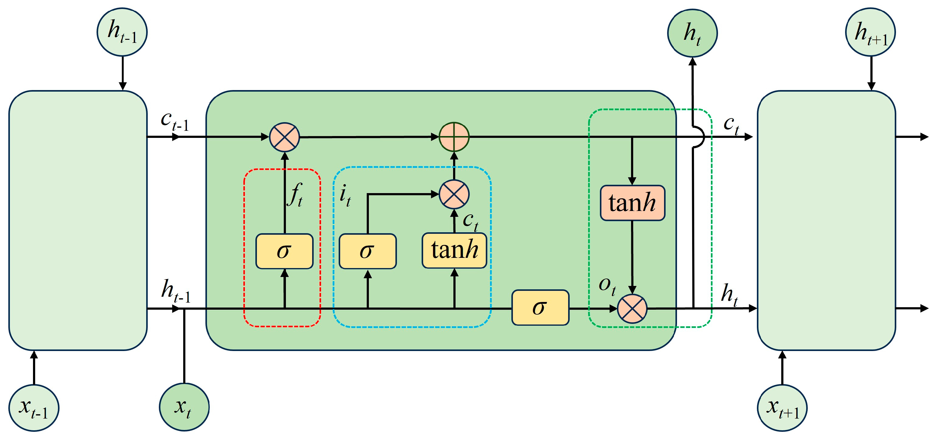
- LSTM neural network
- (2)
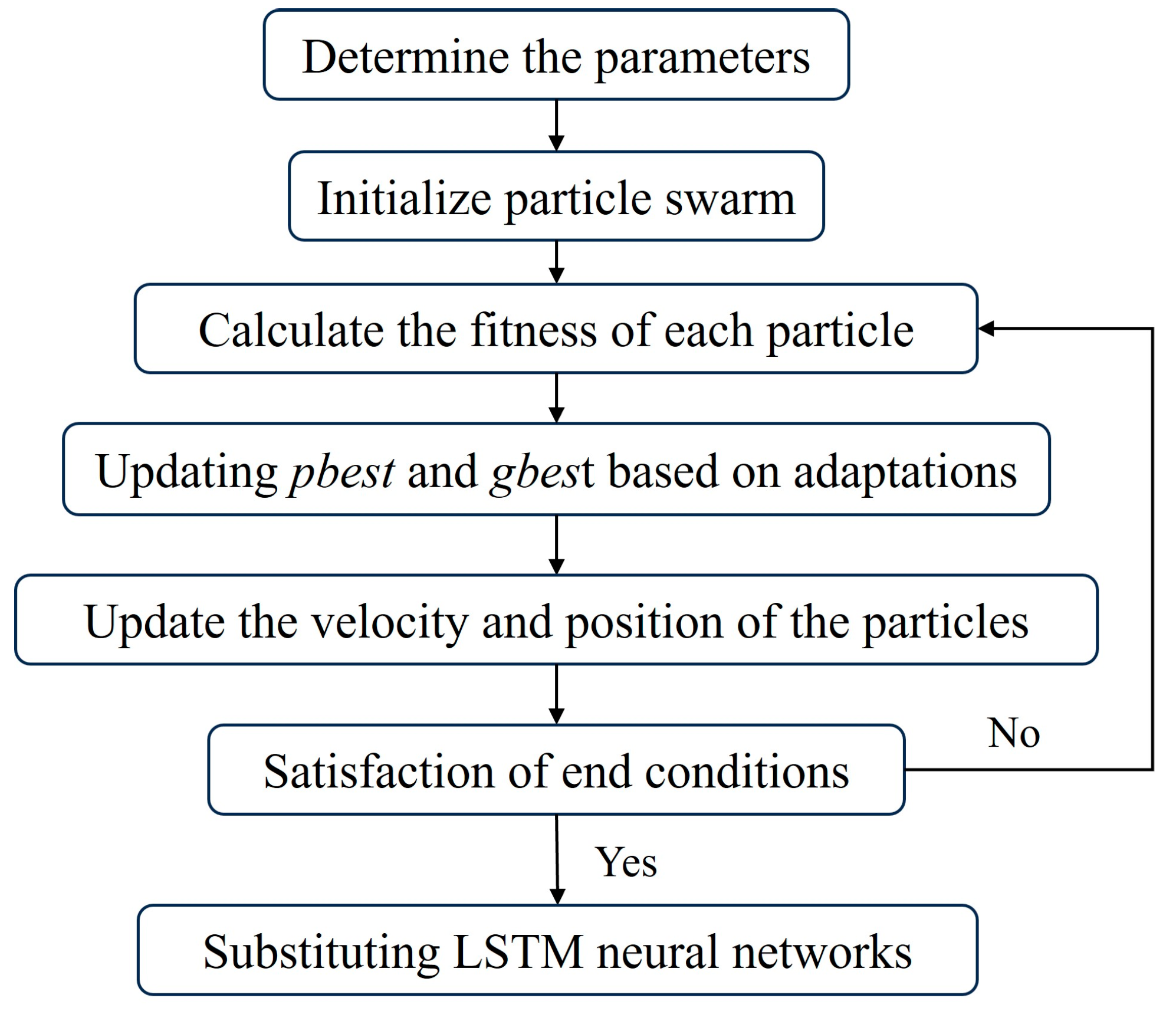
- Particle Swarm Optimization
2.5.3. Predictive Model Performance Evaluation Indicators
2.5.4. Projected Targets
3. Results
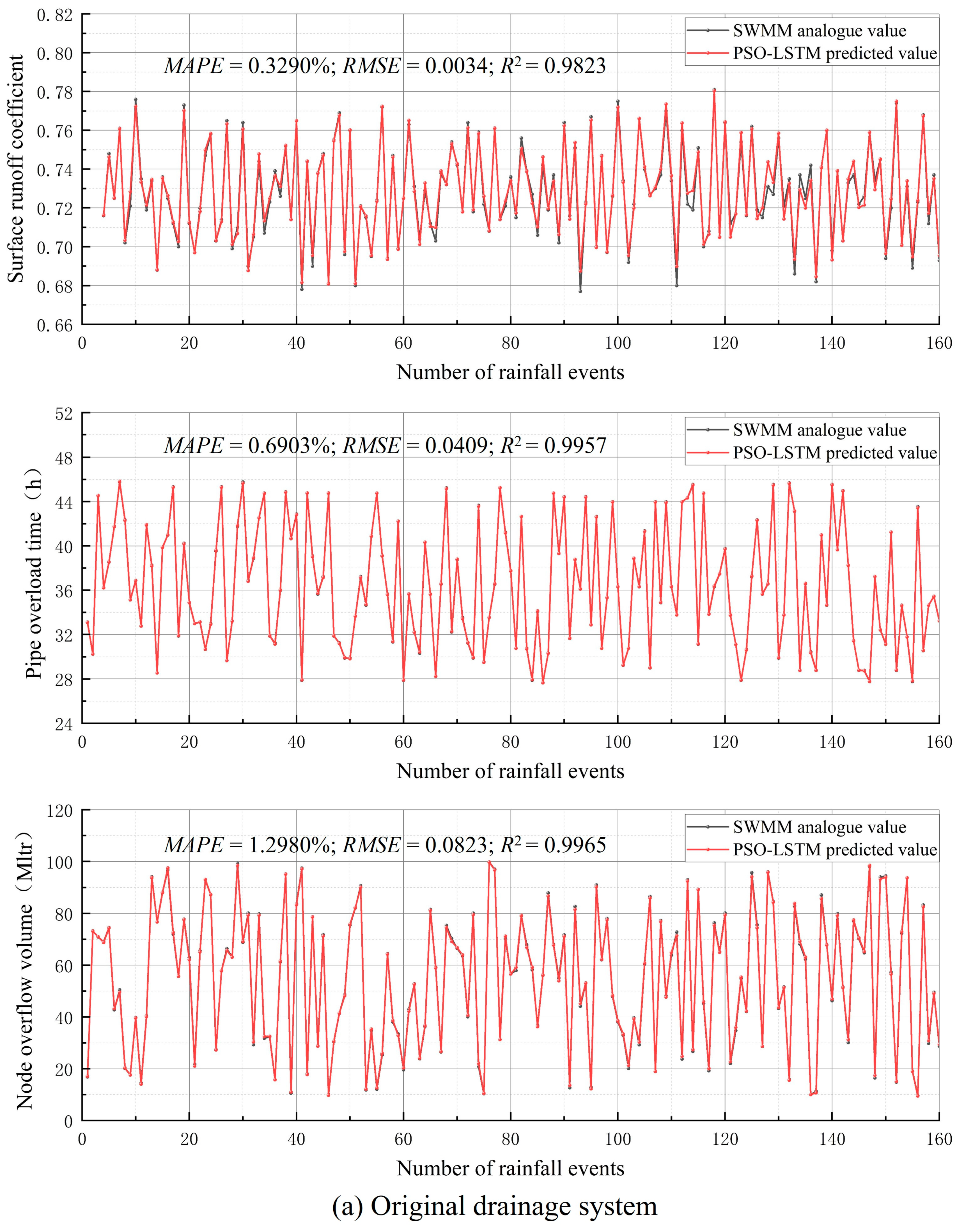
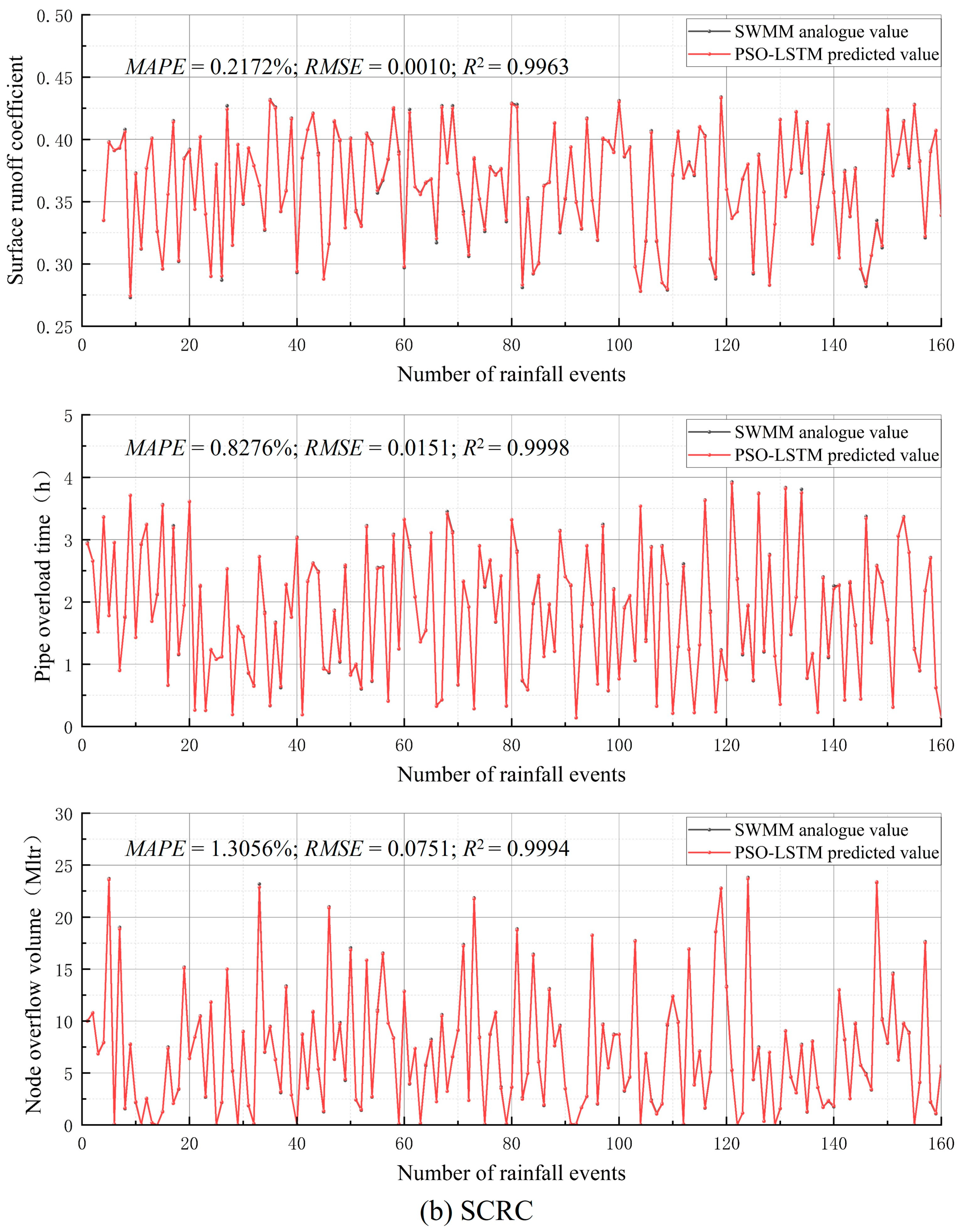
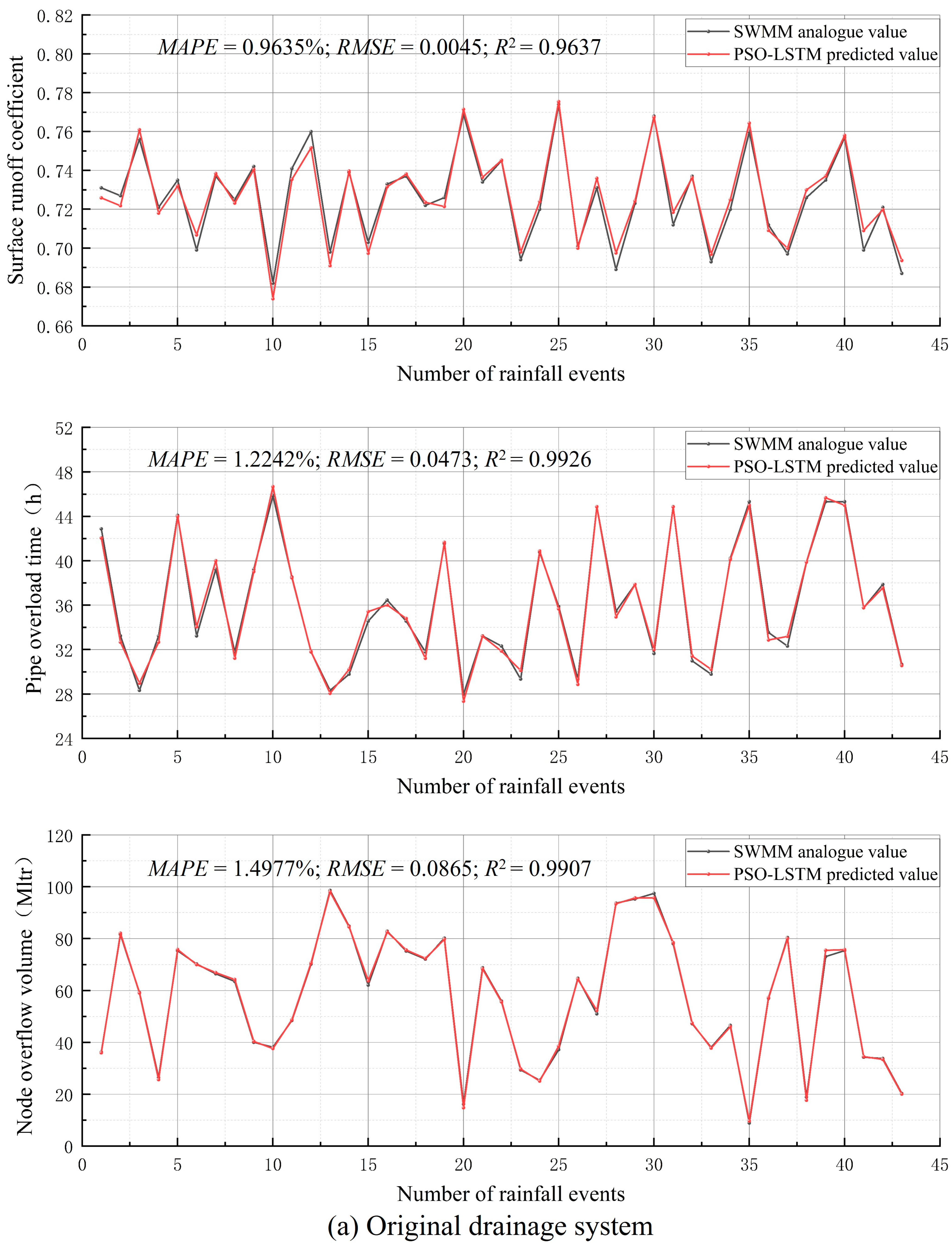
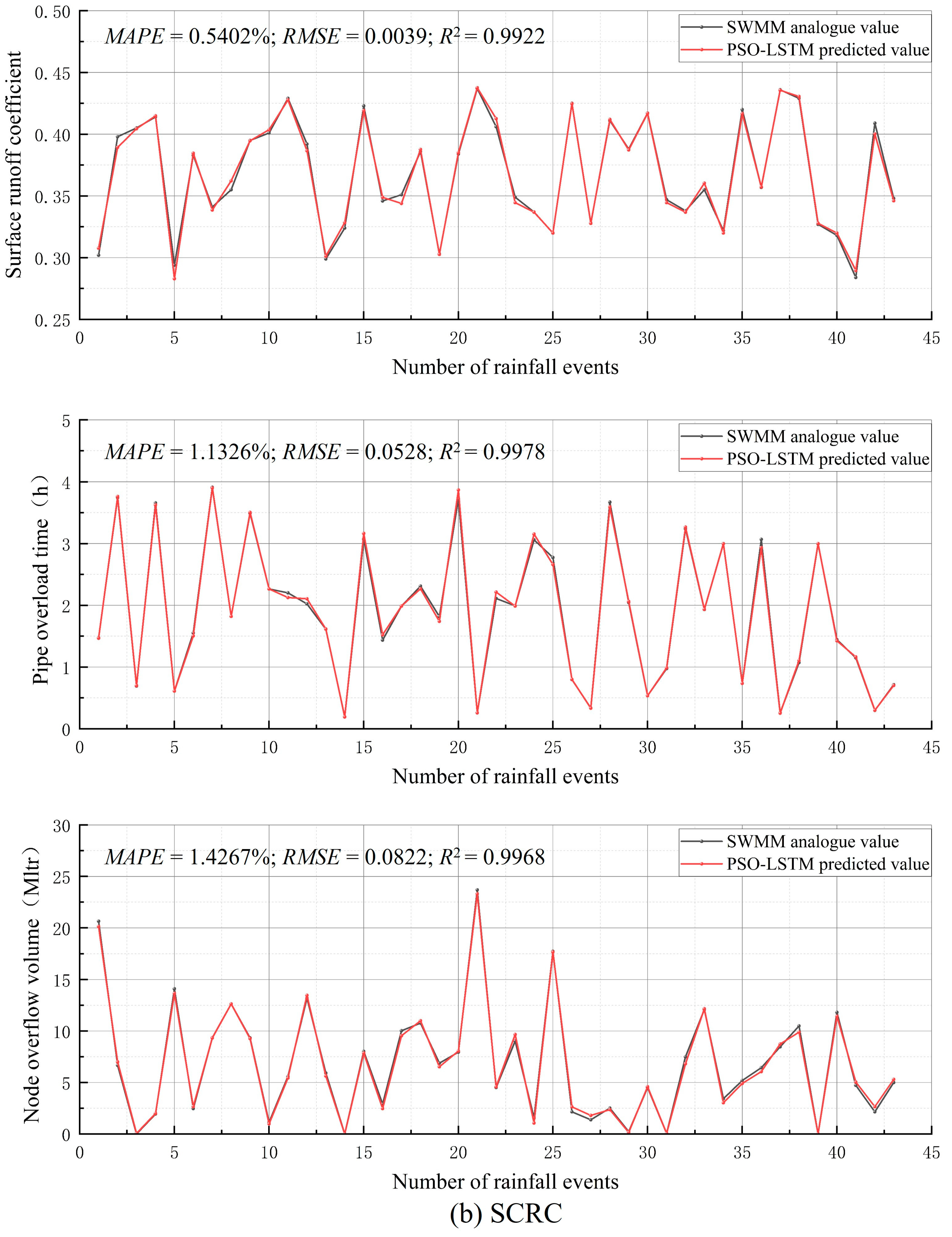
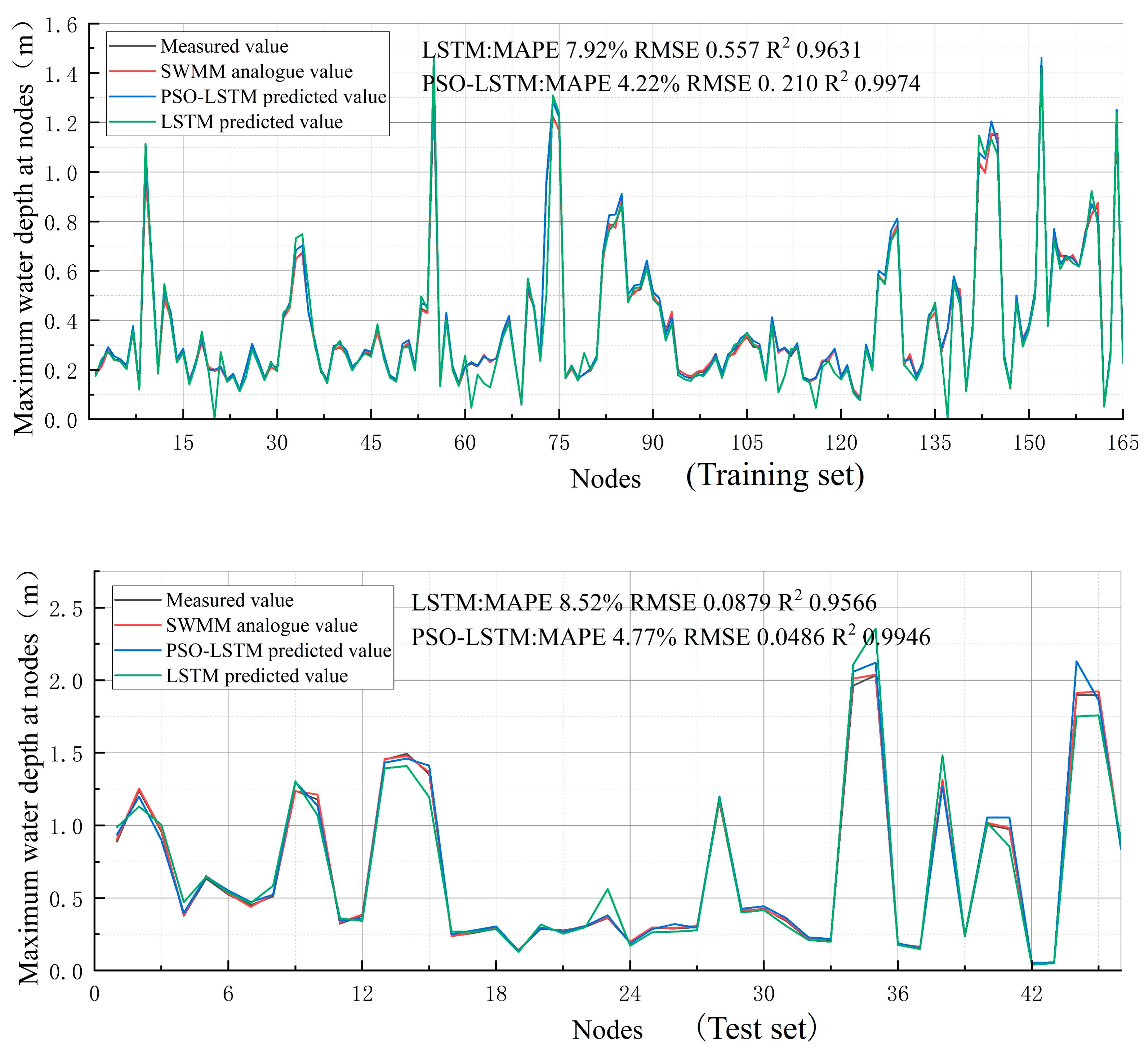
3.1. Predictive Model Performance Analysis
3.2. Comparison of Prediction Models
3.3. Predictive Modeling Results
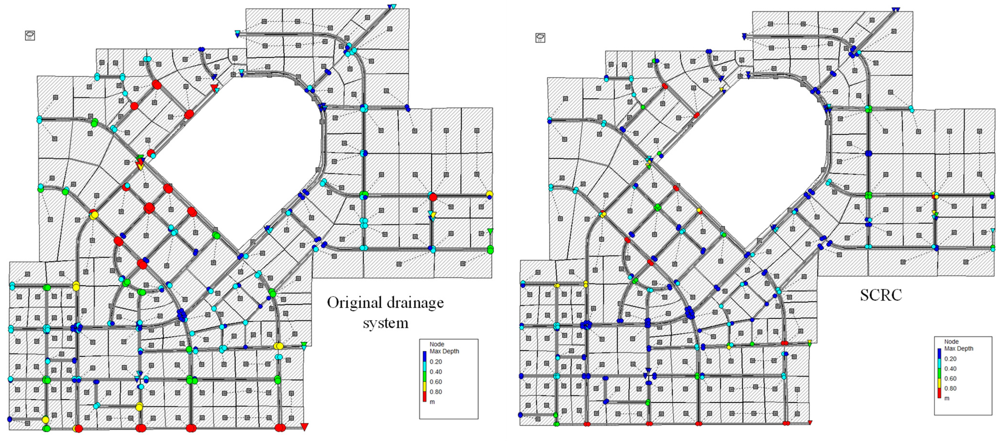
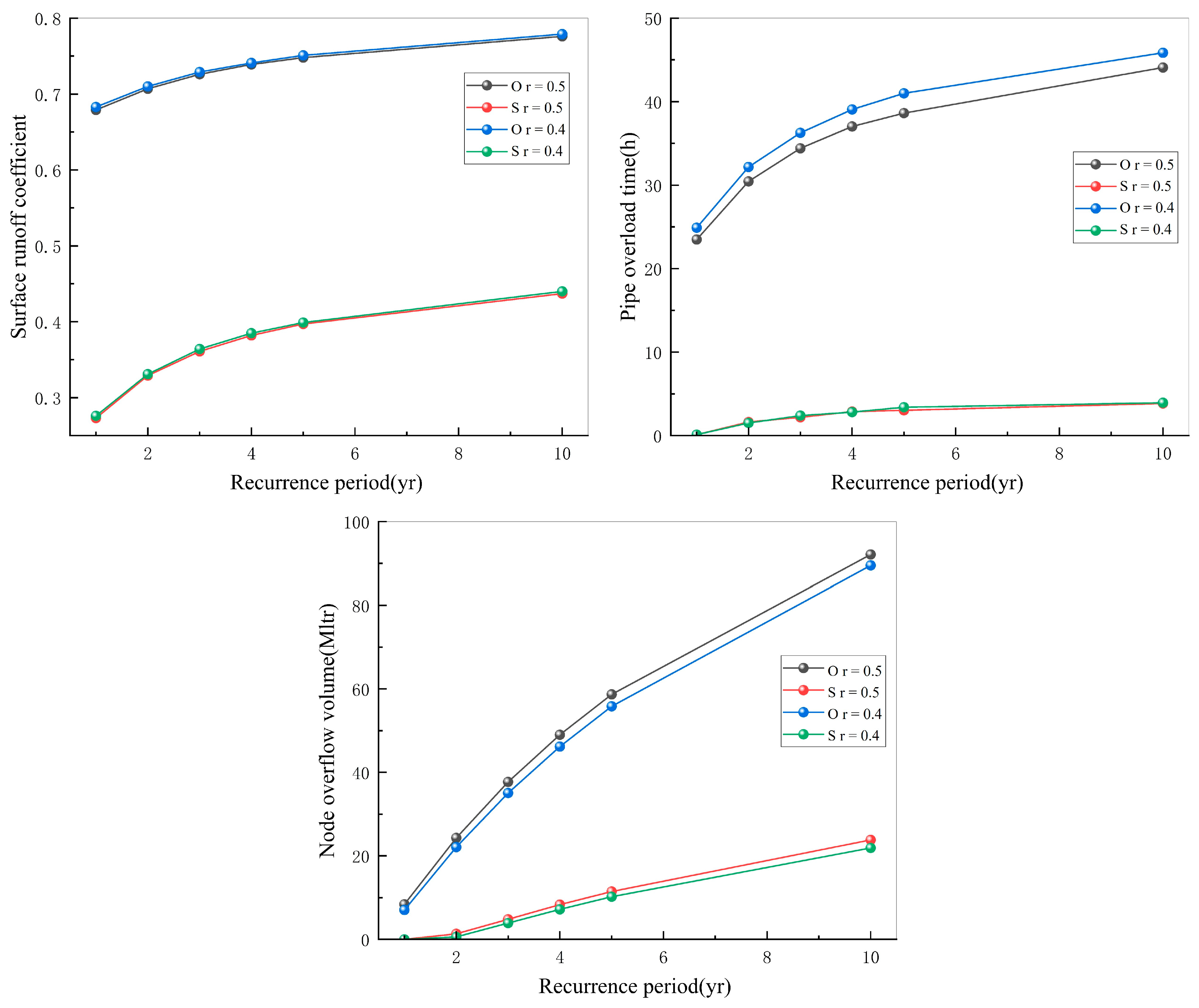
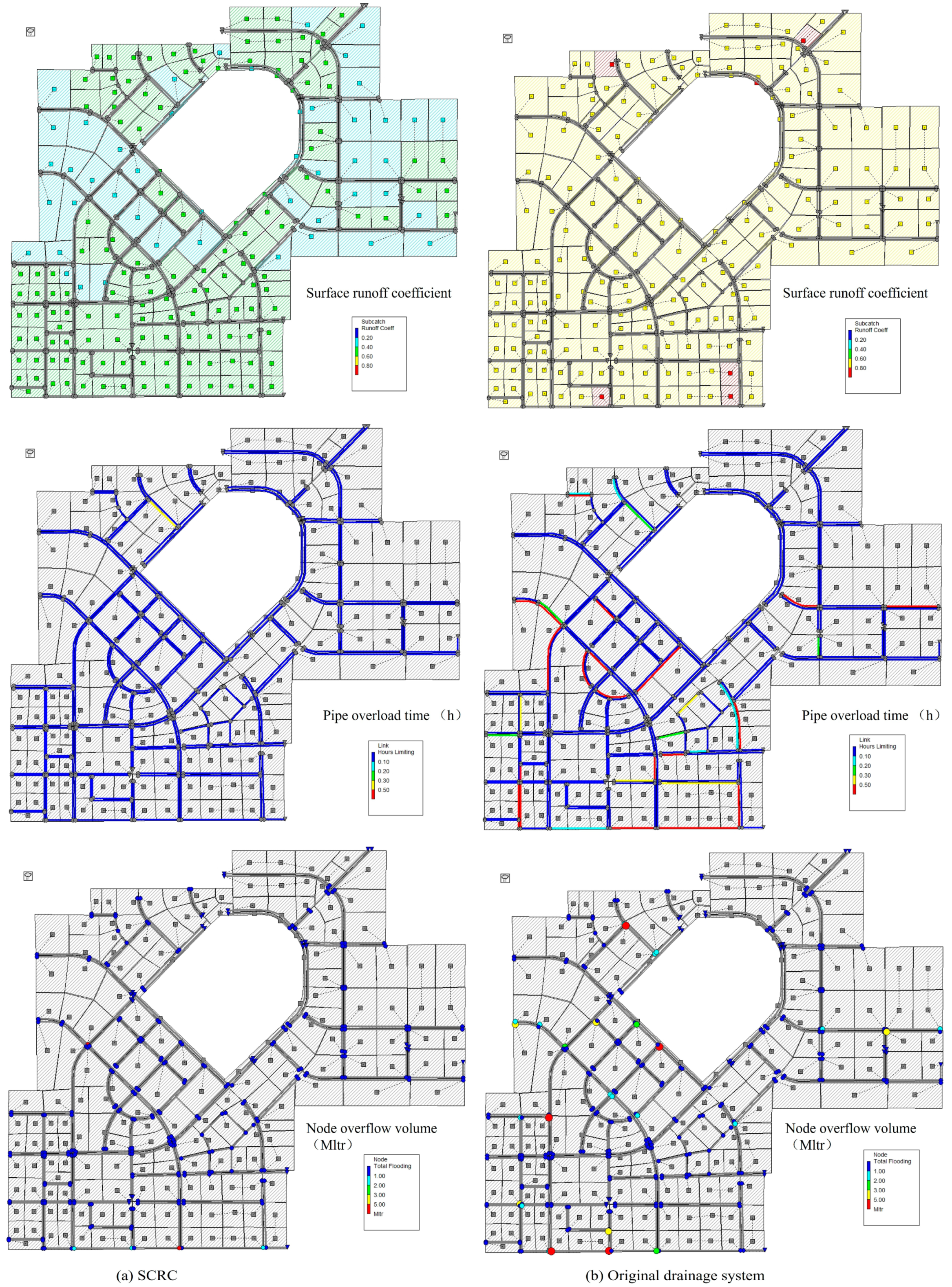
3.4. Effects of SCRC in Alleviating Urban Flooding
4. Discussion
4.1. Effects of Datasets and Hyperparameters
4.2. Neural Networks in Sponge Cities
4.3. Sponge City
5. Conclusions
- (1)
- The PSO–LSTM prediction model provided an excellent prediction performance. The errors between the predicted values and the SWMM simulated values were all very small. The average MAPE of the three flood indicators in the test set was 1.1308%, the average RMSE was 0.0462, and the average R2 was 0.9890, showing that the prediction model displayed an excellent performance.
- (2)
- The SCRC system was effective in mitigating urban flooding. With the extension of the rainfall return period, the reduction effect of the SCRC system on the three urban flooding indicators gradually decreased, but it still showed a good mitigation effect on urban flooding when the rainfall return period was large.
- (3)
- The PSO–LSTM neural network can be effectively used in the field of sponge city flooding, which can provide useful information for the planning and design of future sponge cities.
Author Contributions
Funding
Data Availability Statement
Acknowledgments
Conflicts of Interest
References
- Ma, Y.; Gu, Z.; Wang, T.; Huang, P.; Sheng, J.Y. Analysis of flood control and drainage capacity of hilly city based on SWMM. J. Hohai Univ. 2021, 49, 499–505. [Google Scholar]
- Feng, J.; Wang, Y.; Wu, W.; Zhu, Y. Construction method and application of event logic graph for urban waterlogging. J. Hohai Univ. 2020, 48, 479–487. [Google Scholar]
- Todeschini, S. Hydrologic and environmental impacts of imperviousness in an industrial catchment of northern Italy. J. Hydrol. Eng. 2016, 21, 05016013. [Google Scholar] [CrossRef]
- Handayani, W.; Chigbu, U.E.; Rudiarto, I.; Putri, I.H.S. Urbanization and Increasing Flood Risk in the Northern Coast of Central Java—Indonesia: An Assessment towards Better Land Use Policy and Flood Management. Land 2020, 9, 343. [Google Scholar] [CrossRef]
- Rosenzweig, B.R.; McPhillips, L.; Chang, H.; Cheng, C.; Welty, C.; Matsler, M.; Iwaniec, D.; Davidson, C.I. Pluvial flood risk and opportunities for resilience. Wiley Interdiscip. Rev. Water 2018, 5, e1302. [Google Scholar] [CrossRef]
- Quan, R.S.; Liu, M.; Lu, M.; Zhang, L.J.; Wang, J.J.; Xu, S.Y. Waterlogging risk assessment based on land use/cover change: A case study in Pudong New Area, Shanghai. Environ. Earth Sci. 2010, 61, 1113–1121. [Google Scholar] [CrossRef]
- Billot, R.; Faouzi, N.E.E.; Sau, J.; De Vuyst, F. Integrating the impact of rain into traffic management: Online traffic state estimation using sequential Monte Carlo techniques. Transp. Res. Rec. 2010, 2169, 141–149. [Google Scholar] [CrossRef]
- Ashley, R.; Gersonius, B.; Horton, B. Managing flooding: From a problem to an opportunity. Philos. Trans. R. Soc. A 2020, 378, 20190214. [Google Scholar] [CrossRef]
- Lopes, M.D.; da Silva, G.B.L. An efficient simulation-optimization approach based on genetic algorithms and hydrologic modeling to assist in identifying optimal low impact development designs. Landsc. Urban Plan. 2021, 216, 104251. [Google Scholar] [CrossRef]
- Yin, D.; Chen, Y.; Jia, H.; Wang, Q.; Chen, Z.; Xu, C.; Li, Q.; Wang, W.; Yang, Y.; Fu, G.; et al. Sponge city practice in China: A review of construction, assessment, operational and maintenance. J. Clean. Prod. 2021, 280, 124963. [Google Scholar] [CrossRef]
- Hou, J.; Sun, S.; Wang, Y.; Wang, J.; Yang, C. Comparison of runoff from low-impact development measures in arid and humid cities. Proc. Inst. Civ. Eng. Water Manag. 2022, 175, 135–148. [Google Scholar] [CrossRef]
- Huang, C.L.; Hsu, N.S.; Liu, H.J.; Huang, Y.H. Optimization of low impact development layout designs for megacity flood mitigation. J. Hydrol. 2018, 564, 542–558. [Google Scholar] [CrossRef]
- Khan, M.D.; Shakya, S.; Vu, H.H.T.; Ahn, J.W.; Nam, G. Water Environment Policy and Climate Change: A Comparative Study of India and South Korea. Sustainability 2019, 11, 3284. [Google Scholar] [CrossRef]
- Liu, W.; Chen, W.; Peng, C. Assessing the effectiveness of green infrastructures on urban flooding reduction: A community scale study. Ecol. Model. 2014, 291, 6–14. [Google Scholar] [CrossRef]
- Yang, B.; Zhang, T.; Li, J.; Feng, P.; Miao, Y. Optimal designs of LID based on LID experiments and SWMM for a small-scale community in Tianjin, north China. J. Environ. Manag. 2023, 334, 117442. [Google Scholar] [CrossRef]
- LeCun, Y.; Bengio, Y.; Hinton, G. Deep learning. Nature 2015, 521, 436–444. [Google Scholar] [CrossRef]
- Liu, Y.; Liu, H.; Huo, F.; Liu, Y. Research on spatial and temporal distribution patterns of short-calendar rainstorms based on machine learning. J. Water Resour. 2019, 50, 773–779. [Google Scholar]
- Liu, Y.-Y.; Li, L.; Zhang, W.-H.; Chan, P.-W.; Liu, Y.-S. Rapid identification of rainstorm disaster risks based on an artificial intelligence technology using the 2DPCA method. Atmos. Res. 2019, 227, 157–164. [Google Scholar] [CrossRef]
- Rjeily, Y.A.; Abbas, O.; Sadek, M.; Shahrour, I.; Chehader, F.H. Flood forecasting within urban drainage systems using NARX neural network. Water Sci. Technol. 2017, 76, 2401–2412. [Google Scholar] [CrossRef]
- Zhang, D.; Lindholm, G.; Ratnaweera, H. Use long short-term memory to enhance Internet of Things for combined sewer overflow monitoring. J. Hydrol. 2018, 556, 409–418. [Google Scholar] [CrossRef]
- Razavi, S.; Tolson, B.A.; Burn, D.H. Review of surrogate modeling in water resources. Water Resour. Res. 2012, 48, 1–32. [Google Scholar] [CrossRef]
- Sit, M.; Demiray, B.Z.; Xiang, Z.; Ewing, G.J.; Sermet, Y.; Demir, I. A comprehensive review of deep learning applications inhydrology and water resources. Water Sci. Technol. 2020, 82, 2635–2670. [Google Scholar] [CrossRef] [PubMed]
- Rajaee, T.; Ebrahimi, H.; Nourani, V. A review of the artificial intelligence methods in groundwater level modeling. J. Hydrol. 2019, 572, 336–351. [Google Scholar] [CrossRef]
- Yu, Y.; Si, X.; Hu, C.; Zhang, J. A review of recurrent neural networks: LSTM cells and network architectures. Neural Comput. 2019, 31, 1235–1270. [Google Scholar] [CrossRef]
- Hochreiter, S.; Schmidhuber, J. Long Short-Term Memory. Neural Comput. 1997, 9, 1735–1780. [Google Scholar] [CrossRef]
- Tabas, S.S.; Samadi, S. Variational Bayesian dropout with a Gaussian prior for recurrent neural networks application in rainfall–runoff modeling. Environ. Res. Lett. 2022, 17, 065012. [Google Scholar] [CrossRef]
- Gao, S.; Huang, Y.F.; Zhang, S.; Han, J.C.; Wang, G.Q.; Zhang, M.X.; Lin, Q.S. Short-term runoff prediction with GRU and LSTM networks without requiring time step optimization during sample generation. J. Hydrol. 2020, 589, 125188. [Google Scholar] [CrossRef]
- Kratzert, F.; Klotz, D.; Brenner, C.; Schulz, K.; Herrnegger, M. Rainfall–runoff modelling using long short-term memory (LSTM) networks. Hydrol. Earth Syst. Sci. 2018, 22, 6005–6022. [Google Scholar] [CrossRef]
- Ren, Y.; Zhang, H.; Wang, X.; Gu, Z.; Fu, L.; Cheng, Y. Optimized Design of Sponge-Type Comprehensive Pipe Corridor Rainwater Chamber Based on NSGA-III Algorithm. Water 2023, 15, 3319. [Google Scholar] [CrossRef]
- U.S. Environmental Protection Agency. Storm Water Management Model User’s Manual Version 5.2; U.S. Environmental Protection Agency: Washington, DC, USA, 2022.
- Bach, P.M.; Deletic, A.; Urich, C.; McCarthy, D.T. Modelling characteristics of the urban form to support water systems planning. Environ. Model. Softw. 2018, 104, 249–269. [Google Scholar] [CrossRef]
- Graves, A. Supervised Sequence Labelling with Recurrent Neural Networks; Springer: Berlin/Heidelberg, Germany, 2012. [Google Scholar]
- Kim, K.H.; Youn, H.S.; Kang, Y.C. Short-term load forecasting for special days in anomalous load conditions using neural networks and fuzzy inference method. IEEE Trans. Power Syst. 2000, 15, 559–565. [Google Scholar]
- Graves, A.; Mohamed, A.R.; Hinton, G. Speech recognition with deep recurrent neural networks. In Proceedings of the 2013 IEEE International Conference on Acoustics, Speech and Signal Processing, Vancouver, BC, Canada, 26–31 May 2013; pp. 6645–6649. [Google Scholar]
- Kennedy, J.; Eberhart, R. Particle swarm optimization. In Proceedings of the ICNN’95-International Conference on Neural Networks, Perth, WA, Australia, 27 November–1 December 1995; Volume 4, pp. 1942–1948. [Google Scholar]
- Mousakazemi, S.M.H.; Ayoobian, N. Robust tuned PID controller with PSO based on two-point kinetic model and adaptive disturbance rejection for a PWR-type reactor. Prog. Nucl. Energy 2019, 111, 183–194. [Google Scholar] [CrossRef]
- Ülker, E.D. A PSO/HS based algorithm for optimization tasks. In Proceedings of the 2017 Computing Conference, London, UK, 18–20 July 2017; pp. 117–120. [Google Scholar]
- Jemberie, M.A.; Melesse, A.M. Urban Flood Management through Urban Land Use Optimization Using LID Techniques, City of Addis Ababa, Ethiopia. Water 2021, 13, 1721. [Google Scholar] [CrossRef]
- Cheng, X.; Wang, H.; Chen, B.; Li, Z.; Zhou, J. Comparative Analysis of Flood Prevention and Control at LID Facilities with Runoff and Flooding as Control Objectives Based on InfoWorks ICM. Water 2024, 16, 374. [Google Scholar] [CrossRef]
- Hu, C.; Wu, Q.; Li, H.; Jian, S.; Li, N.; Lou, Z. Deep Learning with a Long Short-Term Memory Networks Approach for Rainfall-Runoff Simulation. Water 2018, 10, 1543. [Google Scholar] [CrossRef]
- Kang, J.; Wang, H.; Yuan, F.; Wang, Z.; Huang, J.; Qiu, T. Prediction of Precipitation Based on Recurrent Neural Networks in Jingdezhen, Jiangxi Province, China. Atmosphere 2020, 11, 246. [Google Scholar] [CrossRef]
- Jin, L.W.; Zhong, Z.Y.; Yang, Z.; Yang, W.X.; Sun, J. Applications of Deep Learning for Handwritten Chinese Character Recognition:A Review. Acta Autom. Sin. 2016, 42, 1125–1141. [Google Scholar]
- Jiang, F.; Fu, Y.; Gupta, B.B.; Liang, Y.; Rho, S.; Lou, F.; Meng, F.; Tian, Z. Deep Learning Based Multi-Channel Intelligent Attack Detection for Data Security. IEEE Trans. Sustain. Comput. 2020, 5, 204–212. [Google Scholar] [CrossRef]
- Lu, N.; Wu, Y.; Feng, L.; Song, J. Deep Learning for Fall Detection: Three-Dimensional CNN Combined With LSTM on Video Kinematic Data. IEEE J. Biomed. Health Inform. 2019, 23, 314–323. [Google Scholar] [CrossRef]
- Zhao, X.; Wang, H.; Bai, M.; Xu, Y.; Dong, S.; Rao, H.; Ming, W. A Comprehensive Review of Methods for Hydrological Forecasting Based on Deep Learning. Water 2024, 16, 1407. [Google Scholar] [CrossRef]
- Sun, H.; Dong, Y.; Lai, Y.; Li, X.; Ge, X.; Lin, C. The Multi-Objective Optimization of Low-Impact Development Facilities in Shallow Mountainous Areas Using Genetic Algorithms. Water 2022, 14, 2986. [Google Scholar] [CrossRef]
- Li, X.-J.; Deng, J.-X.; Xie, W.-J.; Jim, C.-Y.; Wei, T.-B.; Lai, J.-Y.; Liu, C.-C. Comprehensive Benefit Evaluation of Pervious Pavement Based on China’s Sponge City Concept. Water 2022, 14, 1500. [Google Scholar] [CrossRef]


| Rains Return Period (yr) | 2 | 3 | 5 |
| Rainfall depth (mm) | 57.48 | 60.51 | 68.10 |
| Land Use Type | Area (hm2) | Percentage (%) |
|---|---|---|
| Residential land | 299.00 | 26.0 |
| Public administration and public service land | 113.85 | 9.9 |
| Business services facilities land | 136.85 | 11.9 |
| Industrial land | 162.15 | 14.1 |
| Logistics and warehousing land | 148.35 | 12.9 |
| Roads and transportation facility land | 164.45 | 14.3 |
| Serviced land | 21.85 | 1.9 |
| Green space and plaza land | 103.50 | 9.0 |
| Total | 1150.00 | 100 |
| No. | Land Use Type | Combination |
|---|---|---|
| 1 | Residential land, public administration and public service land, and business services facilities land | 50% green roof + 30% permeable pavement +10% vegetative swale + 10% bioretention pond |
| 2 | Industrial land | 40% green roof + 40% permeable pavement +10% vegetative swale + 10% bioretention pond |
| 3 | Logistics and warehousing land | 30% green roof + 50% permeable pavement +10% vegetative swale + 10% bioretention pond |
| 4 | Roads and transportation facility land | 80% permeable pavement +10% vegetative swale + 10% bioretention pond |
| 5 | Green space and plaza land | 40% permeable pavement +30% vegetative swale + 30% bioretention pond |
| Drainage System | Flooding Indicators | MAPE (%) | RMSE | R2 |
|---|---|---|---|---|
| Original drainage system | Surface runoff coefficient | 0.3290 | 0.0034 | 0.9823 |
| Pipe overload time | 0.6903 | 0.0409 | 0.9957 | |
| Node overflow volume | 1.2980 | 0.0823 | 0.9965 | |
| SCRC | Surface runoff coefficient | 0.2173 | 0.0010 | 0.9963 |
| Pipe overload time | 0.8276 | 0.0151 | 0.9998 | |
| Node overflow volume | 1.3056 | 0.0751 | 0.9994 |
| Drainage System | Flooding Indicators | MAPE (%) | RMSE | R2 |
|---|---|---|---|---|
| Original drainage system | Surface runoff coefficient | 0.9635 | 0.0045 | 0.9637 |
| Pipe overload time | 1.2242 | 0.0473 | 0.9926 | |
| Node overflow volume | 1.4977 | 0.0865 | 0.9907 | |
| SCRC | Surface runoff coefficient | 0.5402 | 0.0039 | 0.9922 |
| Pipe overload time | 1.1326 | 0.0529 | 0.9978 | |
| Node overflow volume | 1.4267 | 0.0823 | 0.9968 |
| Node | Measured Value | SWMM Analogue Value | PSO–LSTM Predicted Value | LSTM Predicted Value |
|---|---|---|---|---|
| 26 | 0.179 | 0.182 | 0.188 | 0.175 |
| 27 | 0.217 | 0.213 | 0.228 | 0.244 |
| 28 | 0.278 | 0.276 | 0.292 | 0.273 |
| 29 | 0.243 | 0.239 | 0.255 | 0.241 |
| 30 | 0.239 | 0.235 | 0.242 | 0.232 |
| 31 | 0.209 | 0.211 | 0.218 | 0.203 |
| …… | …… | …… | …… | …… |
| 236 | 0.854 | 0.865 | 0.835 | 0.895 |
| Average error | 1.76% | 4.24% | 8.05% |
| Flooding Indicators | Surface Runoff Coefficient | Node Overflow Volume (Mltr) | Pipe Overload Time (h) | ||||
|---|---|---|---|---|---|---|---|
| Recurrence Period (yr) | SWMM | PSO–LSTM | SWMM | PSO–LSTM | SWMM | PSO–LSTM | |
| 1.5 | 0.301 | 0.298 | 0.671 | 0.677 | 0.11 | 0.108 | |
| 2.4 | 0.34 | 0.338 | 2.994 | 2.899 | 1.898 | 1.891 | |
| 2.6 | 0.349 | 0.351 | 3.149 | 3.151 | 1.923 | 1.913 | |
| 4.5 | 0.39 | 0.387 | 9.833 | 9.828 | 2.945 | 2.932 | |
| 4.8 | 0.392 | 0.39 | 10.677 | 10.674 | 2.979 | 2.968 | |
| 5.5 | 0.405 | 0.403 | 24.265 | 24.263 | 3.127 | 3.11 | |
| Average error | 0.66% | 0.70% | 0.68% | ||||
| Flooding Indicators | Surface Runoff Coefficient | Node Overflow Volume (Mltr) | Pipe Overload Time (h) | ||||
|---|---|---|---|---|---|---|---|
| Recurrence Period (yr) | O | S | O | S | O | S | |
| 1 yr | 0.679 | 0.273 | 8.397 | 0 | 23.487 | 0.11 | |
| 2 yr | 0.707 | 0.329 | 24.313 | 1.343 | 30.45 | 1.632 | |
| 3 yr | 0.726 | 0.361 | 37.712 | 4.799 | 34.409 | 2.193 | |
| 4 yr | 0.739 | 0.382 | 49.004 | 8.311 | 37.021 | 2.869 | |
| 5 yr | 0.748 | 0.397 | 58.701 | 11.455 | 38.625 | 3.021 | |
| 10 yr | 0.776 | 0.437 | 92.12 | 23.828 | 44.081 | 3.847 | |
| Flooding Indicators | Surface Runoff Coefficient | Node Overflow Volume (Mltr) | Pipe Overload Time (h) | ||||
|---|---|---|---|---|---|---|---|
| Recurrence Period (yr) | O | S | O | S | O | S | |
| 1 yr | 0.683 | 0.276 | 7.052 | 0 | 24.907 | 0.11 | |
| 2 yr | 0.71 | 0.331 | 22.094 | 0.591 | 32.178 | 1.517 | |
| 3 yr | 0.729 | 0.364 | 35.051 | 3.916 | 36.265 | 2.384 | |
| 4 yr | 0.741 | 0.385 | 46.194 | 7.181 | 39.063 | 2.81 | |
| 5 yr | 0.751 | 0.399 | 55.828 | 10.205 | 41.006 | 3.398 | |
| 10 yr | 0.779 | 0.44 | 89.52 | 23.89 | 45.858 | 3.929 | |
| Flooding Indicators | Surface Runoff Coefficient | Node Overflow Volume (Mltr) | Pipe Overload Time (h) | ||||
|---|---|---|---|---|---|---|---|
| Recurrence Period (yr) | r = 0.5 | r = 0.4 | r = 0.5 | r = 0.4 | r = 0.5 | r = 0.4 | |
| 1 yr | 59.79% | 59.59% | 100.00% | 100.00% | 99.53% | 99.56% | |
| 2 yr | 53.47% | 53.38% | 94.48% | 97.33% | 94.64% | 95.29% | |
| 3 yr | 50.28% | 50.07% | 87.27% | 88.83% | 93.63% | 93.43% | |
| 4 yr | 48.31% | 48.04% | 83.04% | 84.45% | 92.25% | 92.81% | |
| 5 yr | 46.93% | 46.87% | 80.49% | 81.72% | 92.18% | 91.71% | |
| 10 yr | 43.69% | 43.52% | 74.13% | 73.31% | 91.27% | 91.43% | |
Disclaimer/Publisher’s Note: The statements, opinions and data contained in all publications are solely those of the individual author(s) and contributor(s) and not of MDPI and/or the editor(s). MDPI and/or the editor(s) disclaim responsibility for any injury to people or property resulting from any ideas, methods, instructions or products referred to in the content. |
© 2024 by the authors. Licensee MDPI, Basel, Switzerland. This article is an open access article distributed under the terms and conditions of the Creative Commons Attribution (CC BY) license (https://creativecommons.org/licenses/by/4.0/).
Share and Cite
Ren, Y.; Zhang, H.; Gu, Y.; Ju, S.; Zhang, M.; Wang, X.; Hu, C.; Dan, C.; Cheng, Y.; Fan, J.; et al. Sponge City Drainage System Prediction Based on Artificial Neural Networks: Taking SCRC System as Example. Water 2024, 16, 2587. https://doi.org/10.3390/w16182587
Ren Y, Zhang H, Gu Y, Ju S, Zhang M, Wang X, Hu C, Dan C, Cheng Y, Fan J, et al. Sponge City Drainage System Prediction Based on Artificial Neural Networks: Taking SCRC System as Example. Water. 2024; 16(18):2587. https://doi.org/10.3390/w16182587
Chicago/Turabian StyleRen, Yazheng, Huiying Zhang, Yongwan Gu, Shaohua Ju, Miao Zhang, Xinhua Wang, Chaozhong Hu, Cang Dan, Yang Cheng, Junnan Fan, and et al. 2024. "Sponge City Drainage System Prediction Based on Artificial Neural Networks: Taking SCRC System as Example" Water 16, no. 18: 2587. https://doi.org/10.3390/w16182587
APA StyleRen, Y., Zhang, H., Gu, Y., Ju, S., Zhang, M., Wang, X., Hu, C., Dan, C., Cheng, Y., Fan, J., & Li, X. (2024). Sponge City Drainage System Prediction Based on Artificial Neural Networks: Taking SCRC System as Example. Water, 16(18), 2587. https://doi.org/10.3390/w16182587