Karst Hydrological Connections of Lakes and Neoproterozoic Hydrogeological System between the Years 1985–2020, Lagoa Santa—Minas Gerais, Brazil

Abstract

This study focuses on a complex Brazilian Neoproterozoic karst (hydro)geological and geomorphological area, consisting of metapelitic–carbonate sedimentary rocks of ~740–590 Ma, forming the largest carbonate sequence in the country. At the center of the area lies the Lagoa Santa Karst Environmental Protection Area (LSKEPA), located near the Minas Gerais’ state capital, Belo Horizonte, and presents a series of lakes associated with the large fluvial system of the Velhas river under the influence, locally, of carbonate rocks. The hydrodynamics of carbonate lakes remain enigmatic, and various factors can influence the behavior of these water bodies. This work analyzed the hydrological behavior of 129 lakes within the LSKEPA to understand potential connections with the main karst aquifer, karst-fissure aquifer, and porous aquifer, as well as their evolution patterns in the physical environment. Pluviometric surveys and satellite image analysis were conducted from 1984 to 2020 to observe how the lakes’ shorelines behaved in response to meteorological variations. The temporal assessment for understanding landscape evolution proves to be an effective tool and provides important information about the interaction between groundwater and surface water. The 129 lakes were grouped into eight classes representing the hydrological connection patterns with the aquifers in the region, with classes defined for perennial lakes: (1) constantly connected, (2) seasonally disconnected, and (3) disconnected; for intermittent lakes: (4) disconnected during the analyzed time interval, (5) seasonally connected, (6) disconnected, (7) extremely disconnected, and (8) intermittent lakes that connected and stopped drying up. The patterns observed in the variation of lakes’ shorelines under the influence of different pluviometric moments showed a positive correlation, especially in dry periods, where these water bodies may be functioning as recharge or discharge zones of the karst aquifer. These inputs and outputs are conditioned to the well-developed karst tertiary porosity, where water flow in the epikarst moves according to the direction of enlarged karstified fractures, rock foliation planes, and lithological contacts. Other factors may condition the hydrological behavior of the lakes, such as rates of evapotranspiration, intensity of rainfall during rainy periods, and excessive exploitation of water.

1. Introduction

The Lagoa Santa Karst Environmental Protection Area (LSKEPA) is one of the primary research areas related to archaeology, paleontology, speleology, and hydrogeology in Brazil, located near the state capital of Minas Gerais, Belo Horizonte. The archaeological sites in the Lagoa Santa region are world-renowned, featuring remarkable discoveries, such as the oldest human skeleton fragment in the Americas and a skull that is approximately 11,000 years old, nicknamed Luzia [1].

The lands of the Lagoa Santa region and the karst geomorphology is an interesting feature of the region and represent classic karst study sites in Brazil, where carbonate rocks, upon dissolution, give rise to caves, depressions, sinkholes, and various other unique landforms characteristic of these environments [2,3]. Over the years, various authors have conducted research focusing on the geology, geomorphology, and hydrological dynamics of this region, including [2,4,5,6,7,8,9,10,11,12,13], as well as projects by CPRM (APA Carste Lagoa Santa Project—1998 and Vida Project—2003) and work related to the PAN São Francisco Caves Project [14].

Understanding the hydrological dynamics and groundwater flow in the region is the main focus of various studies, resulting in complex conceptual models for the local karst. Notably, the study by [6] highlights the presence of an extremely active karst aquifer beneath the weathering mantle, where control is primarily exerted by the spatial distribution of the pure limestone occurrences. The recrystallized matrix of these rocks results in very low primary porosity (~3%) [15], where groundwater flows are influenced by secondary and tertiary porosities, such as fractures/faults and karst conduits within the aquifer [7].

The region still lacks studies that can relate the hydrological dynamics between the subterranean and surface karst. In this context, lakes become particularly significant because these karst depressions are crucial for the groundwater recharge of the region’s aquifers. According to [16], the genesis of lakes in karst environments is conditioned by the dissolution of rocks and is strongly influenced by factors that either amplify or diminish this dissolution, such as the structure of the rocks, including their faults and fractures.

Few studies have combined efforts to understand the surface evolution dynamics of these water bodies, but one notable study was conducted by [4], who classified three types of lakes in the region: stable lakes on phyllite; seasonal lakes containing sinkholes at the bottom of dolines in topographically higher areas; and perched lakes on carbonate, at lower elevations. More recent studies use tools such as remote sensing, geoprocessing, aquifer testing, geophysics, isotopic, and meteorological analyses in modeling the evolutionary patterns of karst lakes [17,18,19].

Recently, the region experienced a severe drought, causing many lakes to dry up or significantly reduce their water levels, while others showed no disturbance in their water surface. The lack of knowledge about the hydrological dynamics of these lakes, as well as the need to understand the factors influencing the connection between these water bodies and deep aquifers provided strong incentives for this study.

This work analyzed the hydrological behavior of 129 lakes within the LSKEPA to understand potential connections with the karst aquifer, karst-fissure aquifer and surface porous aquifer, as well as the evolution patterns of their physical environment. Pluviometric surveys and satellite image analysis were conducted from 1984 to 2020 to observe how the lakes’ shorelines behaved in response to meteorological variations. The temporal assessment for understanding landscape evolution proves to be an effective tool and provides information about the interaction between groundwater and surface water.

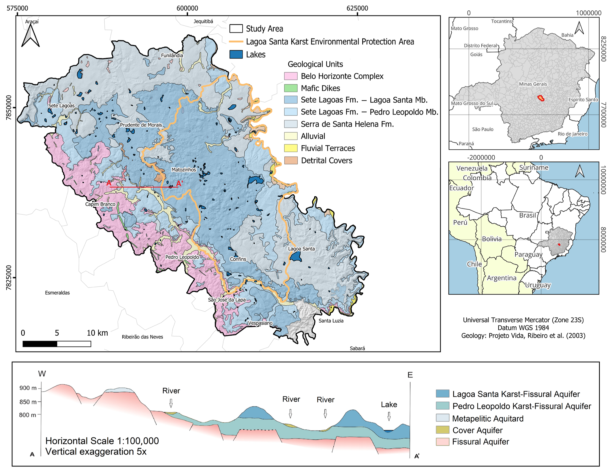
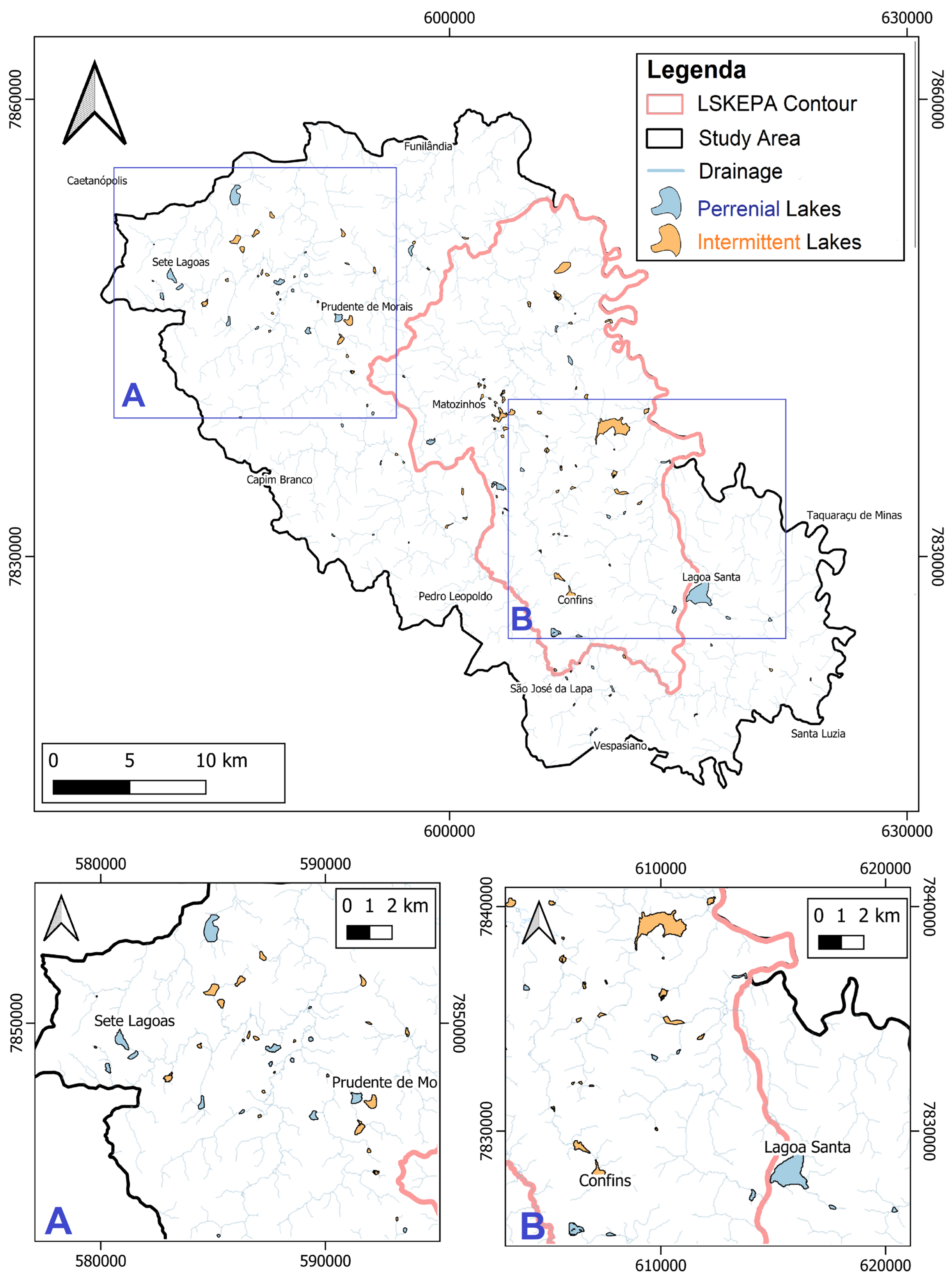
2. Site Description

Referred to by [20] as the “Lagoa Santa Karst Region,” the area of this study has been one of the most extensively studied karst environments since the 19th century, where carbonate and argillo-arenaceous sediments are emplaced giving rise to the Bambuí Group. Located 30 km north of Belo Horizonte, the capital of Minas Gerais state, it covers an area of 1197.5 km² (Figure 1).

Geologically, the study area is regionally located in the central-southern portion of the São Francisco Craton, primarily consisting of Neoproterozoic clastic and carbonate sedimentary cover of the Bambuí Group [23], overlying an Archaean gneissic basement [21] (Figure 1). The craton served as a foundation for the deposition of marine pelitic-carbonate sedimentary packages on a stable epicontinental platform, with a minimum relative age of 630 Ma [24,25].

Locally, the stratigraphy, from bottom to top, features crystalline rocks of the basement, described as an Archaean and Paleoproterozoic Granit-Gneiss-Migmatite Complex (Belo Horizonte Complex) [26], directly overlaid by Neoproterozoic sub-horizontal cover rocks of the Bambuí Group [21,27,28], which in the study area correspond to the Sete Lagoas Formation and the Serra de Santa Helena Formation.

The Sete Lagoas Formation, representing the lower unit of the Bambuí Group, is divided into two members: the Pedro Leopoldo at the base, composed of impure crystalline metacarbonates with fine to medium grain size, intercalated with metapelitic layers; and the Lagoa Santa at the top, featuring pure crystalline metacarbonates with high calcite content and medium to coarse grain size. Both members exhibit partial to total recrystallization of the carbonates [21,27].

The Serra de Santa Helena Formation overlays the Sete Lagoas Formation and consists of metapelites (siltstones, shales, and carbonate lenses), which, even when altered, may display relict structures at the surface [27]. At the top of the stratigraphy, two types of Cenozoic cover rocks are common: detritic–lateritic covers and alluvial covers, occupying higher topographic portions and drainage margins, respectively [21].

The Bambuí Group units in the region exhibit a degree of deformation ranging from moderate to high. Consequently, erosional processes are significantly influenced by fracture families, stratification planes, horizontal foliation, and existing shear zones, which govern the secondary and tertiary porosities of these rocks [29]. The structuring of the rocks is crucial, influencing the widening of conduits along major groundwater flow paths [4,6,30].

The following hydrogeological units are described in the region: granular aquifer of unconsolidated covers, aquiclude in saprolites and pelites of the Serra de Santa Helena Formation, karst aquifer and karst–fissure aquifer in the carbonates of the Sete Lagoas Formation, and fissure aquifer and aquifuge in the domain of gneiss–migmatite granites [31]. A schematic geological section can be observed in Figure 1, representing some of the hydrogeological units. The main aquifer in the region is the karst–fissure aquifer, consisting of the Lagoa Santa Member, which exhibits higher hydrological potential. This is directly related to more intense karstification processes, which promote the widening of fractures and larger conduits [32,33].

In the study area, karst features are widely observed and are important factors in determining the local hydrography, with both fluvial and karstic components [5]. Features such as sinkholes, karst depressions, and caves drain water into subterranean environments, reflecting an evolved karstic environment that affects the recharge and groundwater flow of the aquifers in the region [6,29,33]. Karst depressions play a significant role in the hydrological dynamics of the region and in this study, as many of these can host lakes, whether temporary or permanent. In the Lagoa Santa karst, there is a series of lakes associated with the large Velhas River system, which is part of the São Francisco River Basin.

Many perennial and intermittent karst lakes are present in the region, governed by a complex hydrological dynamic, which can exhibit irregular water level variation patterns, highlighting complex hydrological cycles and behaviors [20,34,35]. The high complexity of the hydrological behavior of these lakes remains a significant question, as these flooded depressions may serve as recharge points for the aquifer or as locations for high-flow springs or resurgence.

Auler, A. et al. [4] classified three types of lakes in the area: stable lakes on phyllite; seasonal lakes containing sinkholes at the bottom of dolines in topographically higher areas; and perched lakes on carbonate, at lower elevations.

Doline-type lakes and perched water table lakes are restricted to limestone rocks, with doline-type lakes primarily occurring in high topographies, at the bottoms of deep karst depressions, and perched water table lakes occurring in low topographic elevations. Generally, lakes on phyllites are stable, while those on limestone have fluctuating water levels, potentially drying up at times. The water level of the latter lakes is related to the amount of precipitation and the permeability of the pedological cover at the lake bottoms [4].

Precipitation control can be decisive for some of these lakes. [36] highlights that climatic variation has direct consequences for the karst region, altering water characteristics, as well as the activity of morphogenetic processes of karst features. Recently, the region experienced a significant drought, resulting in a marked reduction in precipitation and causing many lakes to dry up or significantly reduce their water levels [17,19].

3. Materials and Methods

This study was based on four stages: (1) climatological surveys using data from existing pluviometric stations in the study area from 1984 to 2020; (2) identification of the existing lakes in the area through geoprocessing of Landsat satellite images; (3) detecting the periodicity of these lakes between 1984 and 2020, as well as measuring the water surface dimensions of each lake; (4) evaluating the hydrological behavior of the lakes through various analyses focused on the variation of water levels in different climatological periods over the selected time interval for this study. The stages will be detailed further below.

All maps, rasters, and vector files were geoprocessed in the Universal Transverse Mercator coordinate system, with WGS-1984 Datum, Zone 23S. All geoprocessing activities were carried out using GRASS 7.8.3 tools in the QGIS^® software (Version 3.34.2) [37]. Tables, graphs, and charts were created using Microsoft Excel (Version 2019 MSO) and CorelDRAW (Version Graphics Suite 2024).

3.1. Climatological Survey

Climatological data were obtained from pluviometric stations located in the study area. Raw data from the Sete Lagoas (code 01944052), Pedro Leopoldo (code 01944009), Raul Soares (code 01943049), Vespasiano (code 01943009), Vargem Bonita (code 01944024), Taquaraçu (code 01943023), and Jaboticatubas (code 01943004) stations were downloaded from the HidroWeb portal (snirh.gov.br/hidroweb) of the National Water and Basic Sanitation Agency (ANA).

Data completion was necessary, as the series had some incomplete periods. Statistical correlations between neighboring stations were performed, and the double-mass method was applied. The correlation between two variables was calculated using the Pearson linear coefficient, which, according to [38], represents a mutual relationship between the two variables.

The double-mass method was designed to analyze and group sets of correlated meteorological stations by observing cumulative precipitation diagrams. According to [39], precipitation is less dependent on anthropogenic actions, making it simpler to indicate consistency between two data sets from different meteorological stations.

According to [40], the method involves accumulating monthly or annual precipitation values and plotting them on a graph. The x-axis represents values from the reference station, and the y-axis represents the station to be validated. If the values at both stations are proportional, the graph will be a single line, with the slope defining the proportionality between the two series. If the graph is not a single line, there is a strong indication that the series are not correlatable, there has been a change in the precipitation regime, or the two series belong to different precipitation regimes.

Next, the pluviometric value affecting the area was calculated for each of the studied hydrological years (from October of one year to September of the next year). The Thiessen method [41] was used, which requires the determination of the influence areas for each pluviometer of the selected stations. This method generates a weighted average of the heights recorded by the pluviometers, which is directly proportional to the influence area of the basin, considering the non-uniformity of the spatial distribution of the stations, and does not account for the basin’s topography [40].

Thiessen polygons were drawn in the area for all analyzed hydrological years, from 1984/1985 to 2019/2020, based on the distribution of stations in the area. With the measured precipitation for each hydrological year, historical variations in the precipitation volume affecting the region were estimated, as well as the average precipitation for the 36 years (1984 to 2020).

With the pluviometric inputs calculated for each hydrological year, analyses of data homogeneity and trends were conducted. For homogeneity, the non-parametric Pettitt test [42] was used, which identifies abrupt changes in the temporal data, i.e., a point of discontinuity in the series, according to Equations (1) and (2). The hypotheses to be tested are H₀: F₁(X) = F₂(X) (no change point); H₁: F₁(X) ≠ F₂(X) (change point).

$$U_{t,n}=\sum _{i=1}^t\sum _{j=t+1}^{n}sgn\left(x_t-x_j\right)$$

(1)

$$sgn\left(x_t-x_j\right)=\left\{\begin{array}{c}1if\left(x_t-x_j\right)>0\\ 0if\left(x_t-x_j\right)=0\\ -1if\left(x_t-x_j\right)<0\end{array}\right.$$

(2)

The null hypothesis (H₀) assumes the absence of a change point in the time series. K_t represents the maximum point in the trend change of the series, calculated through the maximum value of U_t,n, which is associated with a significance level (ρ) calculated using Equations (3) and (4). Thus, given a significance level α, if ρ < α, the null hypothesis (H₀) is rejected, where n is the number of years in the time series, ρ is the confidence level, and n is the number of years in the time series. The adopted significance level in this study was 5%.

$$K_t=U_{t,n}=\max \left|U_{t,n}\right|,1\le t<n$$

(3)

$$\rho =2\mathrm{e}\mathrm{x}\mathrm{p}\left({\displaystyle \frac{-6K_n^2}{n^3+n^2}}\right)$$

(4)

The non-parametric Mann–Kendall [43,44] test was conducted to assess the statistical significance (increasing or decreasing) of the climatic time series, distinguishing between natural fluctuation and deterministic trend processes. This method is based on the statistic S, which involves comparing each value of the series with others, always in sequential order, according to Equations (5) and (6).

$$S=\sum _{i=1}^n\sum _{j=1}^{i-1}sgn(x_i-x_j)$$

(5)

$$sgn\left(x_t-x_j\right)=\left\{\begin{array}{c}1if\left(x_i-x_j\right)>0\\ 0if\left(x_i-x_j\right)=0\\ -1if\left(x_i-x_j\right)<0\end{array}\right.$$

(6)

According to [45], the test correlates observation rankings within a time sequence, meaning that it compares each value in the series with previous values in sequential order to determine the statistical variable. In Equation (5), sgn represents the sum of the signs of the pairwise differences of all values in the series (x_i) relative to the remaining values, in sequential order (x_j), where j are the values of the sequential data, and n is the size of the analyzed time series. The results of this summation will vary according to the conditions of Equation (6).

Next, the statistical variance of S, Var(S), is calculated using Equation (7), where n is the number of years in the time series, t is the duration of any period of time, and Σt is the sum of all values of the number of time periods. Equation (8) then calculates the Mann–Kendall statistic Z for this test, where positive values of Z indicate increasing trends, while negative values of Z indicate decreasing trends in the time series. The adopted confidence level was 95%, and the significance level, as in the Pettitt test, was 5%, meaning the probability of rejecting the null hypothesis (H₀) when it is true.

$$Var\left(S\right)={\displaystyle \frac{1}{n}}\left[n\left(n-1\right)\left(2n+5\right)-\sum _{t}t\left(t-1\right)\left(2t+5\right)\right]$$

(7)

$$Z=\left\{\begin{array}{c}{\displaystyle \frac{S-1}{\sqrt{Var\left(S\right)}}}ifS>0\\ 0ifS=0\\ {\displaystyle \frac{S+1}{\sqrt{Var\left(S\right)}}}ifS<0\end{array}\right.$$

(8)

In addition to statistical tests, another approach was taken to observe variations in the temporal rainfall data. Using historical rainfall data and historical mean rainfall, the rainfall cycles occurring throughout the study period were defined. It is known that within a single year, variations between dry and wet periods occur, but the annual rainfall amount, when compared with other annual amounts, can provide important information about how successive years represent a rainfall cycle.

Subsequent years with rainfall values below the historical mean for the analyzed period were grouped into dry or water scarcity cycles. Conversely, sequences of years with rainfall values above the historical mean were grouped into wet cycles. Successive periods where there is no predominant trend of annual rainfall values being consistently above or below the historical mean were categorized as “mixed periods”.

These cycles are of utmost importance when evaluating rainfall data over long intervals, particularly when assessing the temporal behavior of an object, such as the lakes in this study. It becomes apparent that the evaluation of the hydrological dynamics of the lakes is facilitated when examining rainfall variations over shorter intervals. Thus, this study aimed to identify as many rainfall cycles with similar characteristics as possible.

All rainfall data were graphically processed using Microsoft Excel to facilitate the observation and interpretation of the results. The graphs generated from the aforementioned cycles provided resources for creating linear trend lines. A linear trend line is a useful statistical representation for data that increases or decreases at a constant rate [46], and its graphical representation is a straight line that best fits a simple data set. Therefore, each rainfall cycle presented a trend line, representing the variation in growth or reduction of successive rainfall data.

Additionally, within Microsoft Excel, the equations of these trend lines were analyzed. An important piece of information from these equations is the slope coefficient, which relates to the incline of the line and how our data vary successively on a Cartesian plane [46]. The slope coefficients obtained from the trend lines of each rainfall cycle indicate patterns of increasing or decreasing rainfall over the years within a rainfall cycle. Harmonic means of each rainfall cycle were also calculated to compare the rainfall values of each cycle with the historical mean rainfall.

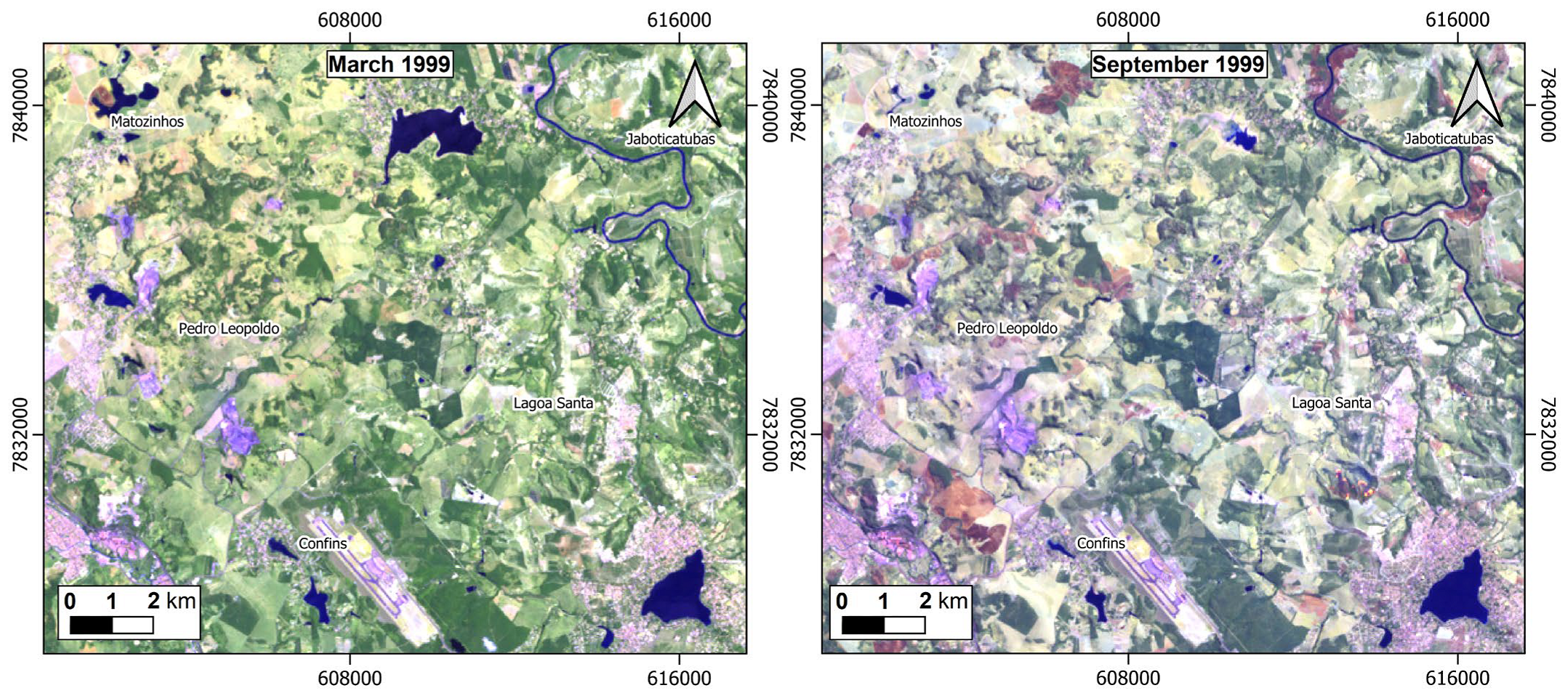
3.2. Identification of Lakes

The processes for identifying lakes outlined by [35] were followed. Initially, land cover scenes from different Landsat satellites [47] for dry and wet seasons of each hydrological year from 1984 to 2020 were selected, while color compositions of spectral bands were created to enhance the contrast between water bodies and other land covers present in the images (Figure 2).

The color compositions served as the basis for conducting a supervised classification, named Region of Interest (ROI), to separate two classes: water bodies and other surfaces. This classification was based on color, texture, tone, and shadows, which are fundamental characteristics to assist in distinguishing the training areas for the predefined classes [48]. Various training areas were selected for each class to achieve greater representativeness of each surface.

Using the Semi-Automatic Classification tool in QGIS software (version 3.34.2), a Maximum Likelihood Classification was performed. This classification calculates the probability that a given pixel belongs to a specific class and labels the class with the highest probability [49]. The result of this step were rasters of classified land cover into water bodies and other surfaces for the wet and dry seasons of all years from 1984 to 2020. These rasters were then converted into vector files to facilitate data handling and to exclude water bodies with linear patterns, which more closely resemble rivers rather than lakes, the focus of this study.

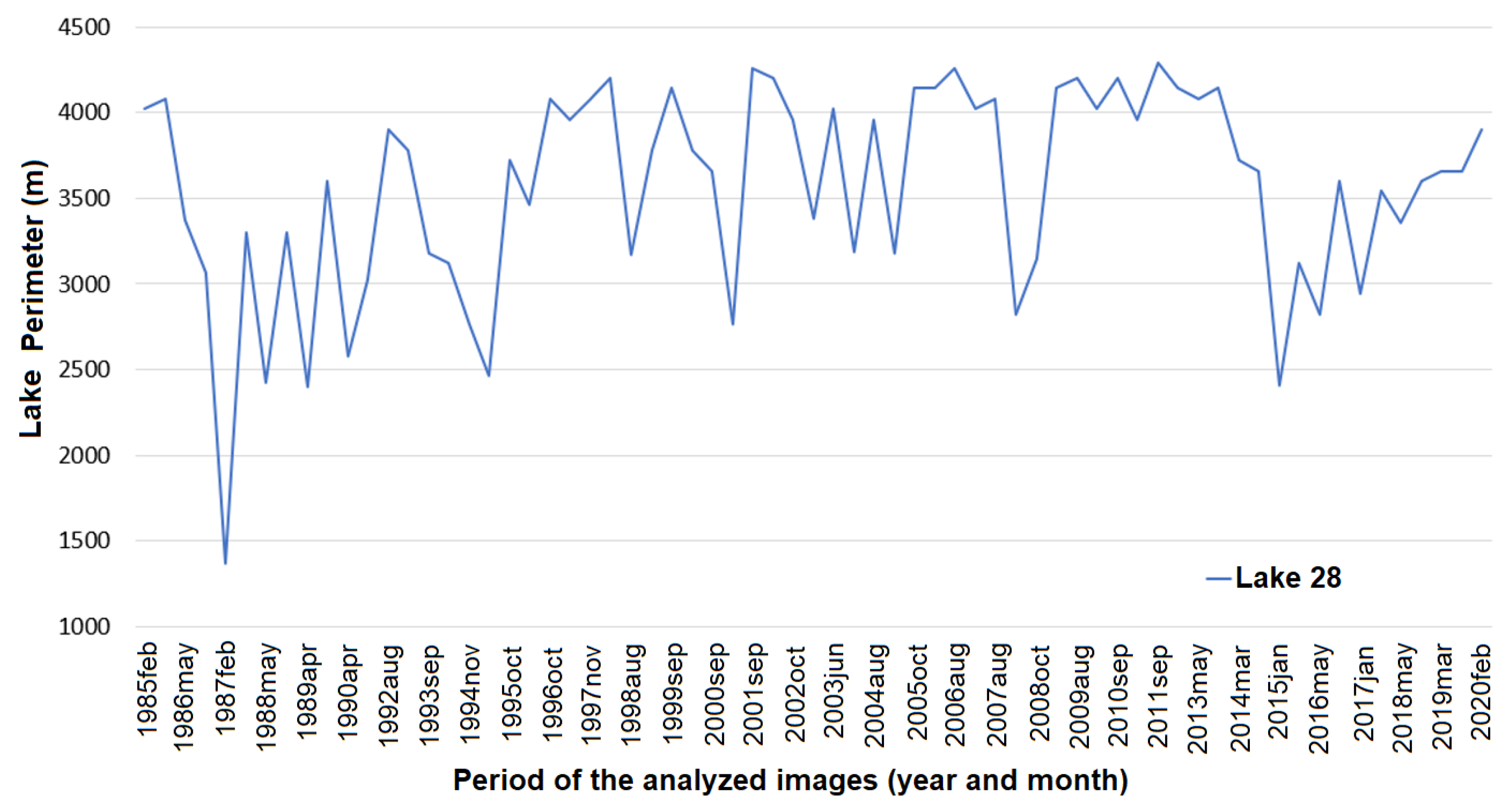
3.3. Periodicity of the Lakes

With the water bodies defined for the dry and wet seasons between the hydrological years of 1984 and 2020, the behavior of all the lakes regarding their periodicity of appearing full or dry was observed. This step defined which lakes had perennial or intermittent behavior. Perennial lakes are those that never dried out during the study period. Intermittent lakes are those that existed in the 1980s and show a periodic behavior of having or not having water in different years between 1984 and 2020. At this stage, the perimeter of these lakes was also calculated, corresponding to the length of the outermost edge of the water bodies, varying according to their size and shape. The perimeter values were obtained using the Calculate Geometry/Perimeter tool from the attribute table of the QGIS vector files.

3.4. Assessment of Hydrological Behavior

For the analysis of hydrological behavior, the perimeter data of the lakes for each hydrological year were initially processed graphically using Microsoft Excel. Graphs were created to represent each lake and how numerically whether its water body expanded or contracted during the study period. This step involved defining the averages and perimeters of the lakes, indicating what would be considered their normal behavior over the years (Figure 3).

The perimeter data were analyzed in relation to the previously defined rainfall cycles, and new trend lines representing the successive variation in perimeters were observed for each of the dry, wet, or mixed cycles. The angular coefficients in this analysis were important, as they represent how much the lakes expanded or contracted during each rainfall cycle. The sum of these coefficients can be interpreted as reflecting the changes in the water body of a lake and be compared with the average perimeter of each lake to observe the behavior of each one over the analyzed years. Contractions of less than 5% of the average lake size were considered minor, while contractions greater than 5% were considered significant. A flowchart of this step can be seen in Figure 4.

To observe the hydrological behavior of the lakes during abrupt changes in precipitation, a new approach was proposed. The perimeters of the lakes were analyzed in relation to changes in rainfall cycles, highlighting how each lake’s behavior was affected by significant changes in precipitation. The period chosen was between the transition from the rainy cycle to the dry cycle, an event that occurs only once in the temporal interval used. The end of the rainy cycle was set to 2011, and the start of the dry cycle was set to 2012. Graphically, precipitation was compared with the perimeter variations each lake might exhibit.

This method proved more effective for perennial lakes compared to intermittent ones, likely due to the potential connection with groundwater bodies that perennial lakes might have. Perennial lakes are more likely to be connected to aquifers and receive constant groundwater replenishment. Therefore, lakes that do not show a disturbance in their water body in response to abrupt changes in precipitation may be connected lakes. Conversely, lakes affected by precipitation and showing perimeter changes may not be as connected to the regional groundwater system. Intermittent lakes are frequently dry, and precipitation is crucial for them to hold water. Hence, a comprehensive analysis across all research years was used for these lakes to identify moments when their hydrological behavior changed.

The analysis focused on perennial lakes, comparing the two proposed approaches described in this section: the first related to the final behavior of the lakes over the years, identifying which expanded and which contracted over time, as well as quantifying this growth or reduction; the second related to the lake’s behavior during the transition between a rainy cycle and a period of precipitation scarcity, demonstrating possible connections or disconnections between perennial lakes and groundwater. If these approaches are validated, it is expected that lakes with a greater connection to the aquifer will show minimal contraction or even expansion of their water body by the end of this study. Conversely, disconnected lakes should show greater contraction of their water body over the successive years.

Unlike perennial lakes, analyzing trend lines and their angular coefficients for intermittent lakes was not useful. This is because almost all intermittent lakes exhibit negative trend lines, as these lakes are often empty during various periods over the studied years—a defining characteristic of intermittent lakes. Thus, the analysis of intermittent lakes’ hydrological behavior was conducted by graphically examining their water bodies (perimeter) over the full study period (36 years) and comparing it with precipitation. Lakes with similar behavior were grouped into classes based on their hydrological connection.

4. Results and Discussion

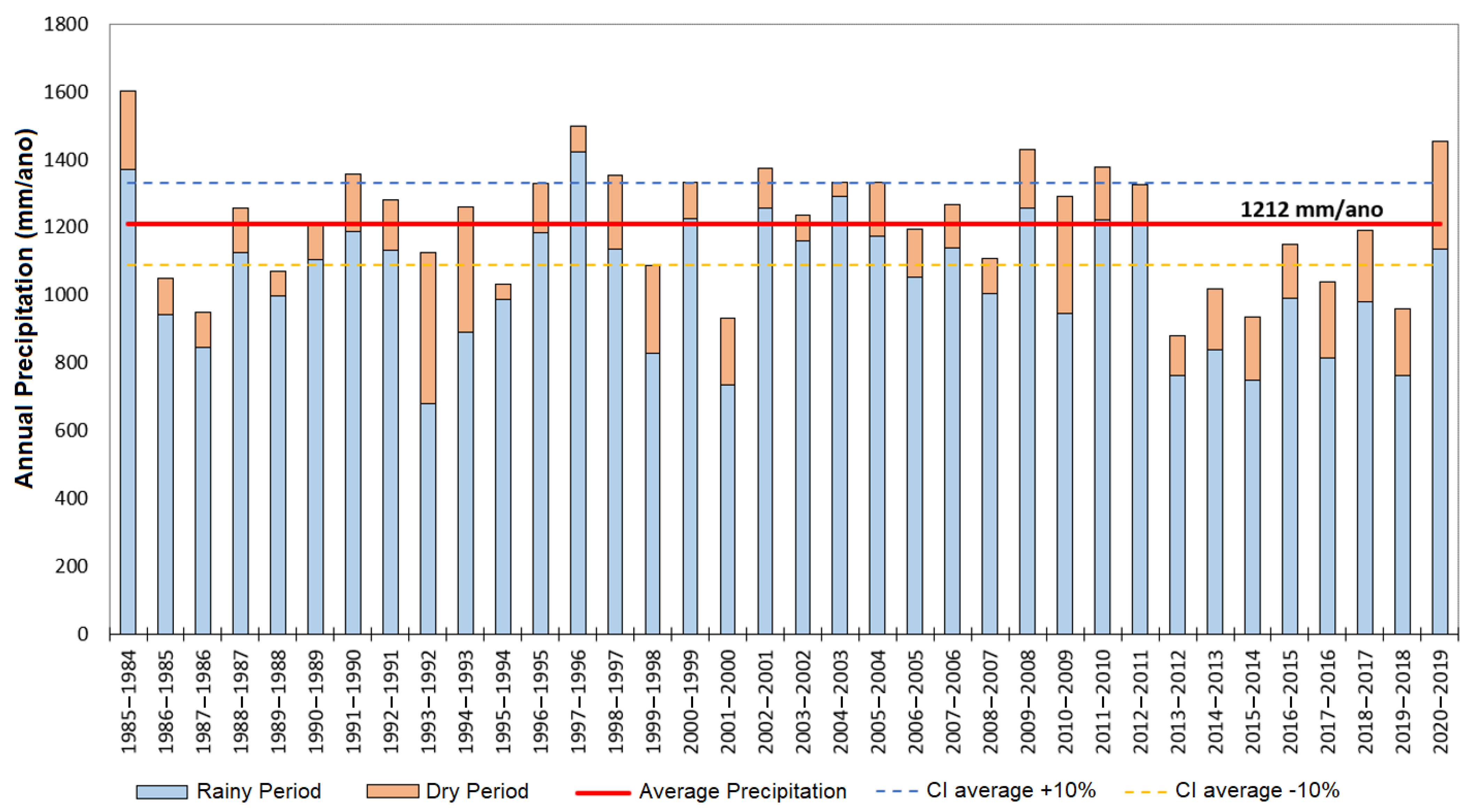
4.1. Historical Precipitation

Using data from the pluviometric stations, a graph was created to represent the historical annual average precipitation for all hydrological years between 1984–1985 and 2019–2020 (Figure 5).

With the annual averages calculated, a new calculation was performed to represent the historical precipitation average over the years studied, resulting in a value of 1212 mm. This value is of great importance, as it helps identify hydrological years with low precipitation and those with high precipitation, representing significant cycles of flooding and water scarcity over recent years.

A total of 20 hydrological years had precipitation above the historical average for the analyzed period, much of which occurred between the hydrological years 2001–2002 and 2011–2012. Conversely, 16 hydrological years had precipitation below the historical average, with the most notable period being between the years 2012–2013 and 2018–2019. The negative confidence interval, represented by 10% below the average of 1212 mm, showed a good fit to the data, without significantly altering the behavior of the analyzed hydrological years.

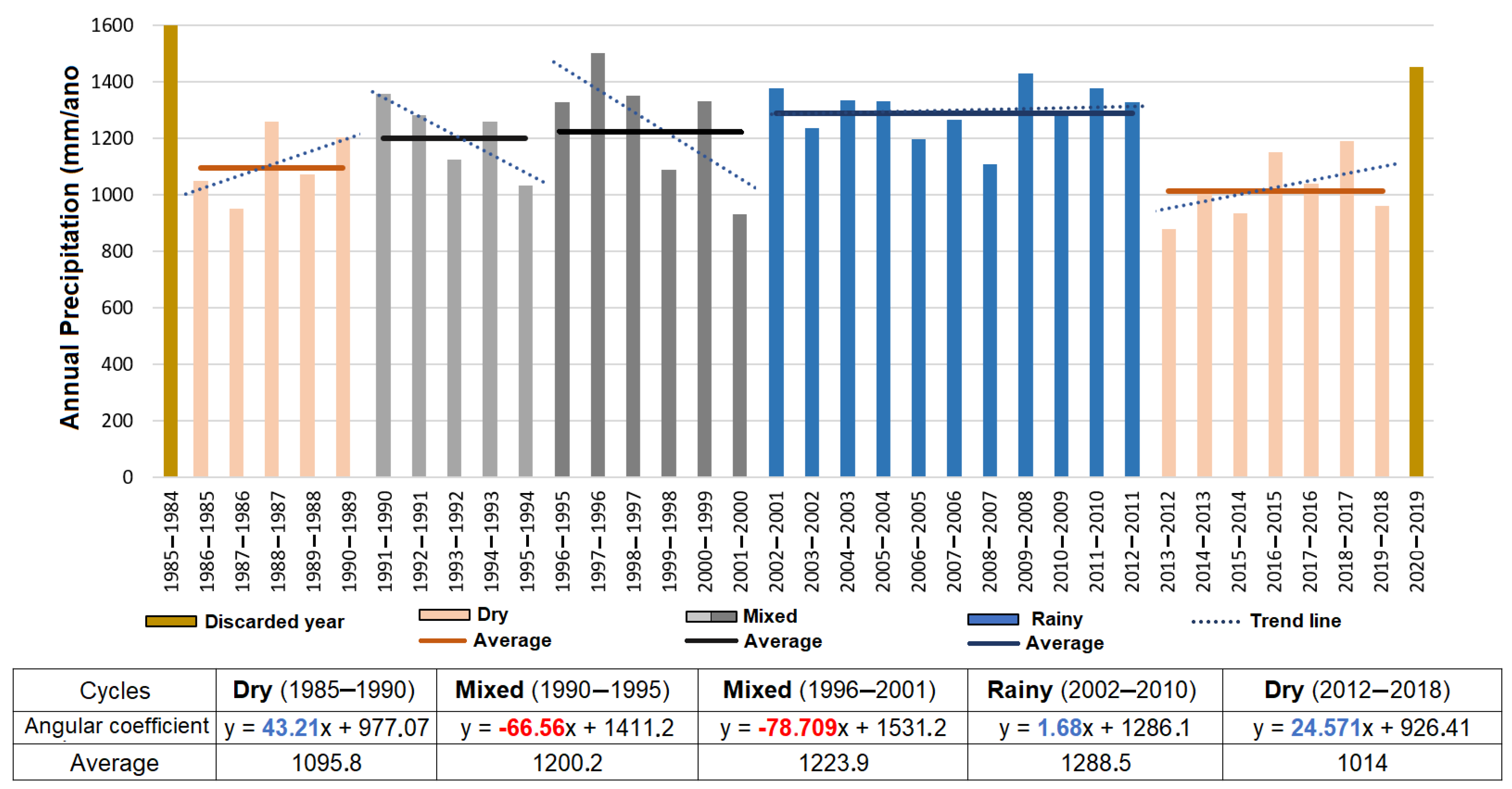
4.2. Precipitation Cycles

Climatic homogeneity was tested (Pettitt’s test) for the time series of hydrological years between 1984–1985 and 2019–2020, indicating that there are no change points in precipitation throughout the selected interval. Based on the 5% significance level, H₀ is accepted; that is, there was no change point, as ρ > α = 0.05 was found in these parameters, showing a homogeneous behavior. The Mann–Kendall trend test results indicated similar behavior to Pettitt’s test for precipitation, where H₀ is accepted (ρ > α = 0.05), showing no significant trend (

Table 1. Statistical nonparametric results based on homogeneity (Pettitt’s test) and trend analysis (Mann–Kendall test).

Method	Parameter	Precipitation
Pettitt’s test	K	124
	t	28
	p-value (two-tailed) alpha	0.39 0.05
	Interpretation a	Accept H0
Mann–Kendall trend test	Kendall’s tau	−0.06
	S	−38
	Var(S)	5390
	p-value (two-tailed)	0.61
	alpha	0.05
	Interpretation b	Accept H0

Notes: ^a Two hypotheses: H₀ = no change point; H₁ = change point. Based on the significant level of 5%, if ρ < α = 0.05, H₀ is rejected (change point); if ρ > α = 0.05, H₀ is accepted (no change point). ^b Two hypotheses: H₀ = no trend; H₁ = significant rising or declining trend. Based on the significant level of 5%, if ρ < α = 0.05, H₀ is rejected (there is a trend in the data); if ρ > α = 0.05, H₀ is accepted (no trend in the data).

).

The statistical tests, therefore, were not effective in diagnosing significant changes in precipitation or in identifying increasing or decreasing trends in the rainfall data. Consequently, an alternative approach was proposed to identify the nuances in precipitation data over the years.

Based on the historical precipitation record and the historical average, the cycles of rainfall and water scarcity were defined. Hydrological years consecutive to the historical average precipitation (1212 mm/year) were grouped into rainfall cycles, while subsequent hydrological years with values below the historical average were categorized as drought cycles. The years that showed inconsistency with the historical average were grouped into “mixed” cycles (Figure 6). The first and last hydrological years of the data group were excluded due to the inability to analyze the behavior of the years preceding and following these years.

Throughout the historical series, five cycles were identified, ranging from 5 to 11 years in duration. The historical series begins with a 5-year dry period, one of the shortest cycles in the set (1984/1985 to 1989/1990), featuring only one hydrological year (1987–1988) above the historical average. This is followed by two mixed cycles, one lasting 5 years (1990/1991 to 1994/1995) and the other lasting 6 years (1995/1996 to 2000/2001).

This sequence of hydrological years hardly represents a grouping of years of water scarcity or abundance, as the years do not show a pattern of consecutive years above or below the average precipitation. Thus, they were categorized into mixed precipitation cycles. The decision to separate into two mixed cycles rather than one was due to the precipitation fluctuations observed, with each mixed cycle starting with high precipitation values that decrease over the years. The precipitation variations within these cycles are crucial for understanding the hydrological behavior of the lakes.

Following this, a major wet cycle occurs, the longest in the set, lasting 11 years (2001/2002 to 2011/2012). This cycle had only 2 years (2005–2006 and 2007–2008) with precipitation below the historical average. The final cycle is a drought cycle lasting 7 years (2012/2013 to 2018/2019). During this cycle, all hydrological years were below the historical precipitation average, showing very low precipitation volumes; this significant reduction in precipitation in the region is also noted in the works of [19,50,51].

The first (1984–1985) and last (2019–2020) hydrological years of the analyzed interval were excluded, as including them in any cycle would not have been coherent due to the unknown behavior of the years preceding the chosen interval and those following the study period. The wet, dry, and mixed periods were graphically treated to observe the trend lines of each cycle and the harmonic mean precipitation values that encompass only the precipitation values of each period (Figure 7).

The average rainfall for the two dry periods was well below the historical average (1212 mm/year) previously represented, with the first dry period showing 1095.8 mm/year and the second dry period 1014 mm/year. In contrast, the wet period (2001 to 2012) had an average of 1288.5 mm/year, significantly above the historical average (1212 mm/year), which is expected for a wet precipitation cycle.

Observing the average for each of the mixed cycles reveals an interesting pattern: the average rainfall during the years of each cycle is close to the historical precipitation average (1212 mm/year). This reflects the nature of these periods, characterized by variations of high and low rainfall over the years, similar to what is observed when analyzing the entire study period (1984 to 2020). The first mixed period had an average of 1200.2 mm/year, and the second had an average of 1223.9 mm/year.

The trend lines for each cycle type (dry, wet, and mixed) show similar behaviors. During dry periods, the trend lines exhibit a positive trend, indicating an annual increase in precipitation within these cycles. This suggests that the beginning of precipitation scarcity cycles is more severe, with precipitation tending to approach the historical average over time. The annual increase in precipitation over the cycle is 43.2 mm/year (the first dry cycle) and 24.5 mm/year (the second dry cycle).

Mixed cycles exhibit the opposite behavior of dry cycles, with trend lines showing negative values. This indicates that these cycles start with higher precipitation values and show a reduction in precipitation throughout the cycle, with a decrease of 66.5 mm/yr (the first mixed cycle) and 78.7 mm/year (the second mixed cycle).

Finally, the wet cycle shows a constant trend line, indicating a well-defined cycle, with most of its hydrological years marked by high precipitation values. The trend line is positive, showing an increase of 1.6 mm/year over the cycle.

4.3. Lake’s Identification and Periodicity

Based on the analysis of the water body behavior during this period, 129 lakes were classified in two main types: 40 perennial lakes, which had water bodies in both the rainy and dry seasons of all hydrological years; and 89 intermittent lakes, which showed significant variation in water bodies between the dry and rainy seasons, sometimes becoming completely dry in the dry season or remaining dry for several hydrological years before reappearing (Figure 8).

The perimeter value of each lake was also determined, representing the length of the outermost edge of the water bodies for each image used, varying according to their size and shape. This measurement provided the basis for the subsequent stages of this research.

4.4. A Lake’s Water Behavior

The perimeter variation was observed, as well as the trend lines of this variation within the precipitation cycles, and angular coefficients were calculated, representing how the lakes expanded and contracted in each of the precipitation cycles. The sum of these angular coefficients can be interpreted as the change in the water body of a lake over the 36-year period covered in this study.

Figure 9 illustrates the perimeter variation of one of the perennial lakes, where the table represents the trend line equation for the perimeter variation of its water body across each analyzed cycle, along with the sum of the angular coefficients of this variation in all cycles. For visualization, one lake was chosen, and this measurement was conducted for 40 perennial lakes and 89 intermittent lakes in the region of focus.

In Figure 9, the behavior of perennial lake number 23 and how its perimeter varied from 1985 to 2020 can be observed. As a perennial lake, it never dried up during the analyzed interval; however, it showed significant variation in its water body, with many variations recorded during the previously defined wet and dry cycles. During the first dry cycle, the lake showed what is considered a normal variation, where its water body expanded and contracted according to the precipitation variations between dry and wet seasons within a hydrological year. At the end of this cycle, the angular coefficient generated by the trend line equation indicated a loss of 3.56 m in its water body.

The two subsequent mixed cycles had distinct influences on the lake’s perimeter. During the first mixed cycle, the lake experienced a contraction of 18 m, while in the second mixed cycle, it expanded by 2.72 m.

The wet cycle between 2002 and 2011 represented a significant positive variation in the lake’s perimeter, which may be related to the higher precipitation occurring in this cycle. During this cycle, the lake reached its largest water body within the analyzed interval, totaling 780 m in perimeter, and this value was maintained for several years. At the end of this cycle, the trend line equation indicated that the lake had an expansion of 8.73 m throughout the wet cycle.

Finally, the lake faced a last dry cycle, where its water body drastically reduced, reaching values of 425 m during the dry season of 2017, the period of greatest contraction for the lake in the analyzed interval. At the end of this cycle, the lake began to expand again, but not enough to show a positive variation over the cycle. The trend line represented a reduction of 24 m for the lake throughout the analyzed years. The sum of all angular coefficients obtained for each cycle resulted in a total contraction of 34.15 m for the lake over the years analyzed.

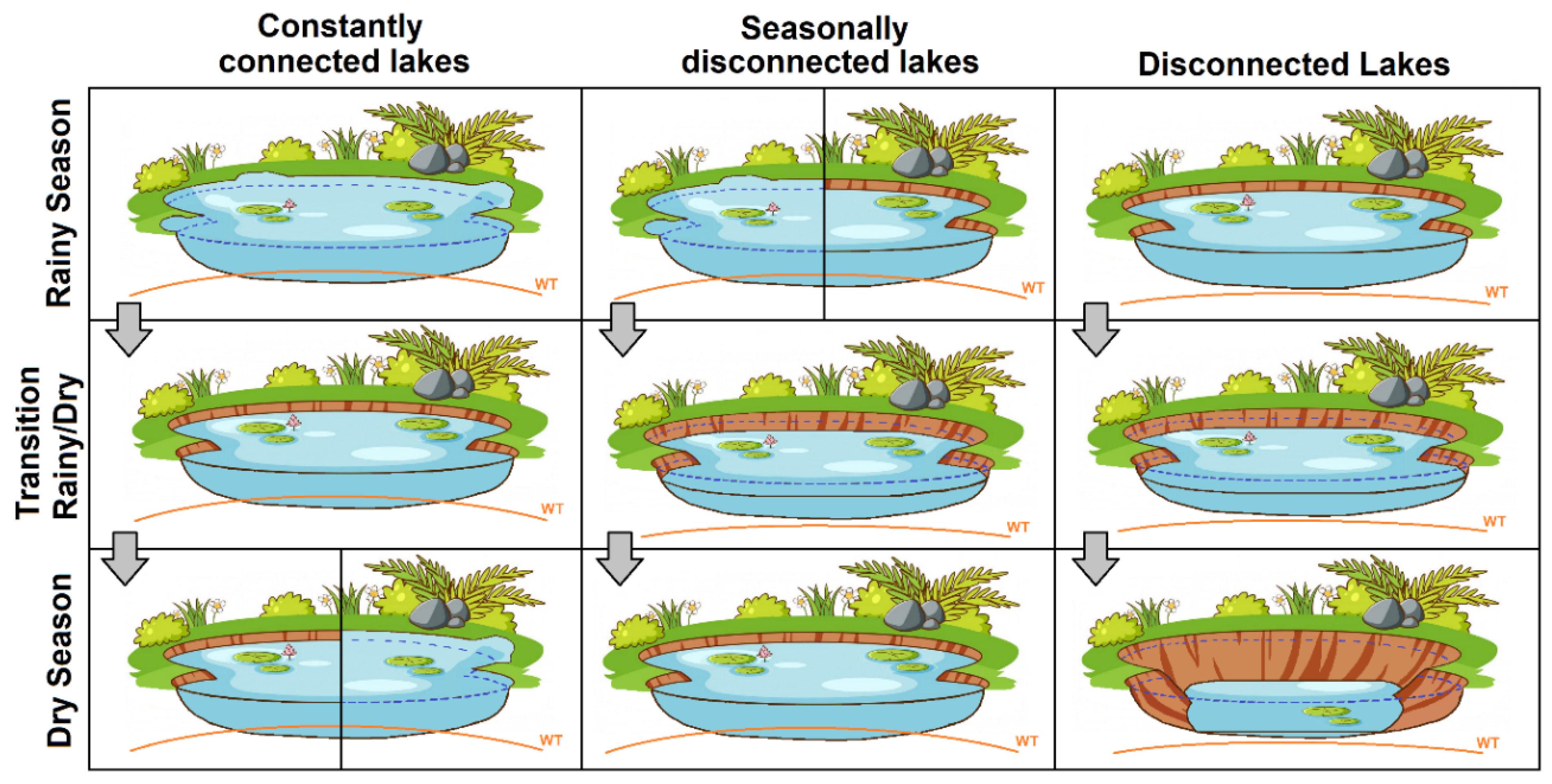
4.5. Lake Classes of Hydrological Connection

The previous data provided the foundation to define the hydrological connection classes representing perennial and intermittent lakes, which exhibit similar behavior in response to perimeter variation related to changes in precipitation patterns. Different approaches were used to analyze the hydrological connection for perennial lakes and intermittent lakes. The results for each type of lake will be discussed below, starting with perennial lakes and followed by intermittent lakes.

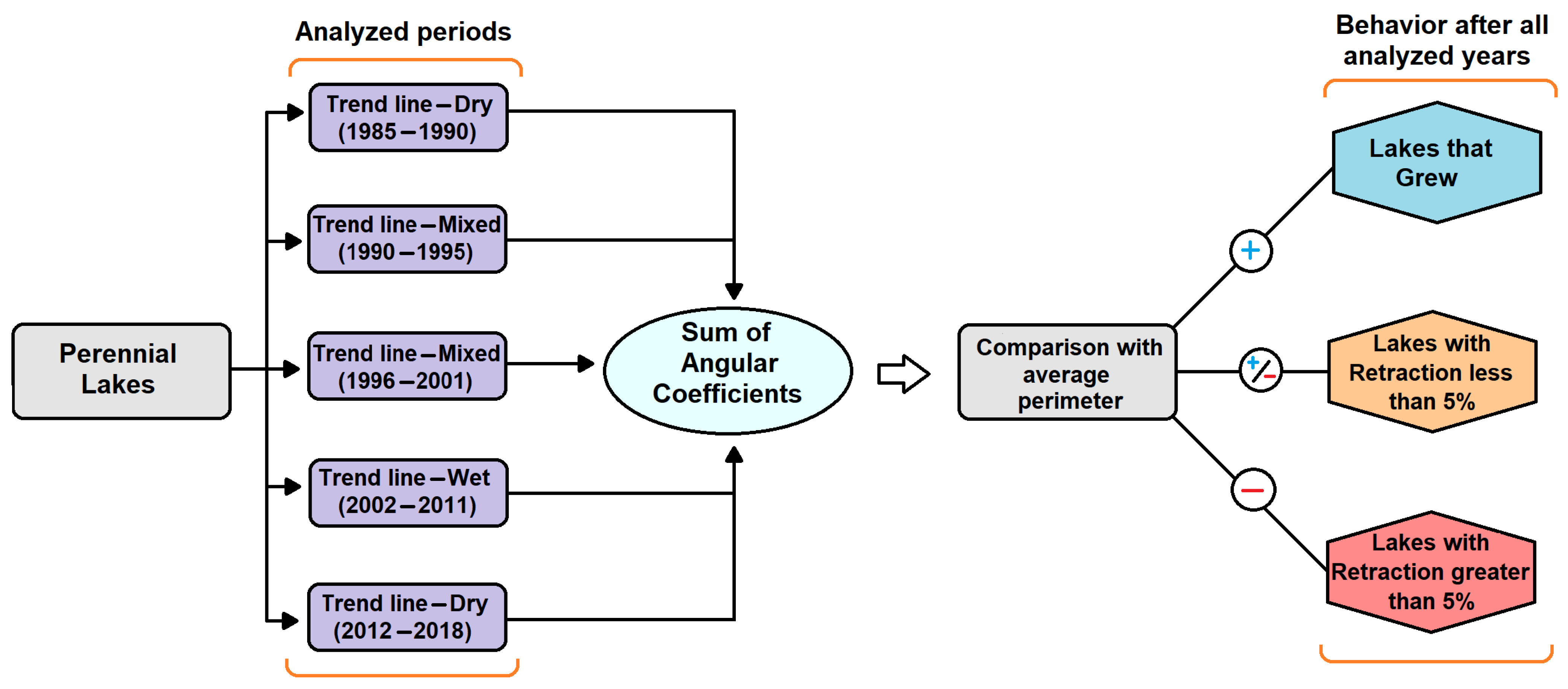
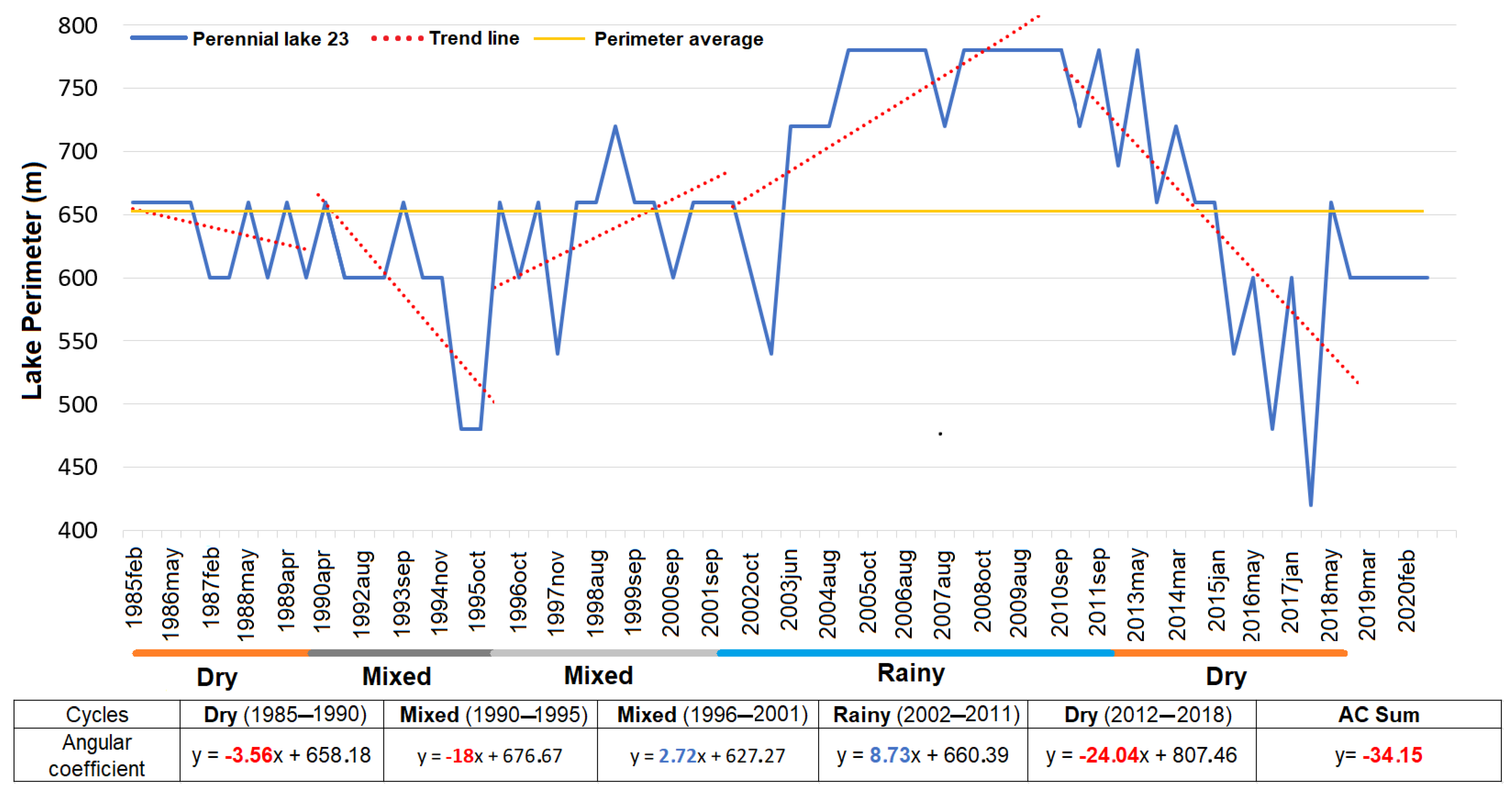
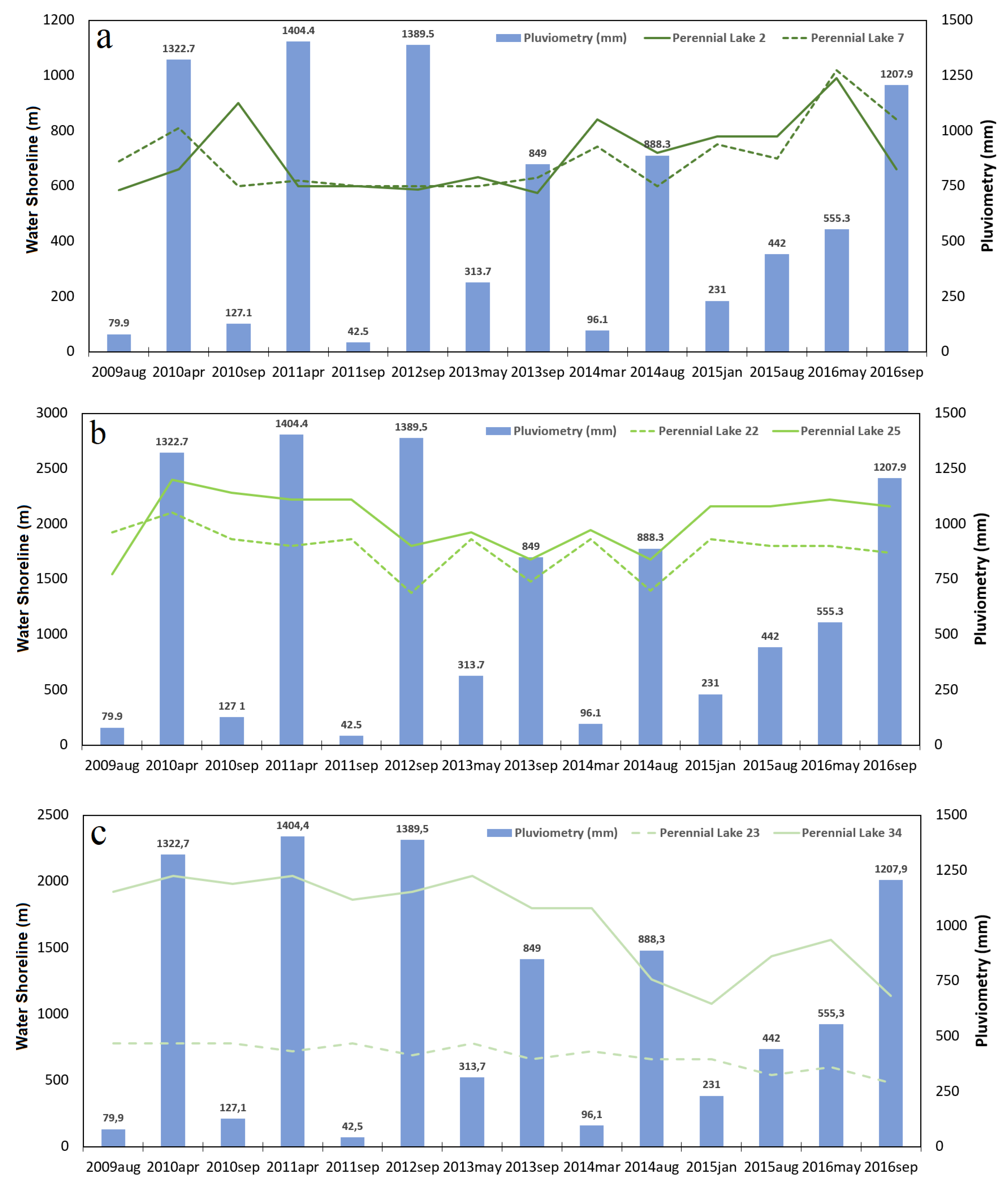
4.5.1. Perennial Lakes—Analysis of Angular Coefficients

For the analysis of the hydrological connection of the 40 perennial lakes, the sum of the angular coefficients for all the previously defined precipitation cycles was first observed. These sums indicated which lakes grew or shrank during the 36 years analyzed in this study. Interpreting this behavior in relation to the evolution of their water bodies is crucial for identifying lakes that are connected to the aquifer. These lakes, regardless of precipitation variations, were replenished by groundwater and experienced an increase in their water surface. Conversely, lakes that might be disconnected could be losing water through infiltration and percolation, unable to maintain their water levels within their depressions solely through precipitation.

The equations of the trend lines and their angular coefficients, as well as the sum of these coefficients, are detailed in

Table A1. Perennial lakes and their perimeter variation behaviors in each of the rainfall cycles defined in this study, as well as the final behavior after all the analyzed years. Note: Red numbers indicate lake contraction, and blue numbers indicate lake expansion.

Perennial Lakes	Trend Lines							Behavior after All Analyzed Years
	Dry (1985–1990)	Mixed (1990–1995)	Misto (1996–2001)	Dry (1985–1990)	Mixed (1990–1995)	Somatório de Todos Coeficientes Angulares	Dry (1985–1990)	Mixed (1990–1995)	Lagoas Que Diminuíram Menos de 5%	Dry (1985–1990)
1	y = −4.8112x + 767.94	y = 7x + 758.33	y = 813.33	y = −4.7678x + 835.29	y = −3.2253x + 804.12	y = −5.79	784		x
2	y = −11.224x + 773.95	y = −24.467x + 718.33	y = 7.1x + 580.94	y = 5.9556x + 593.59	y = 18.231x + 584.77	y = −4.39	669		x
3	y = 0.979x + 318.64	y = −2x + 335.56	y = 0.5x + 330.83	y = −0.5676x + 335.95	y = −0.4396x + 332.31	y = −1.52	328		x
5	y = −30.927x + 718.94	y = −2.1667x + 414.17	y = 9.3706x + 370.76	y = 3.7131x + 454.5	y = −1.4286x + 551.54	y = −21.42	493			x
6	y = −34.213x + 1008.5	y = 2.3333x + 660.78	y = 16.157x + 578.89	y = −1.9628x + 791.54	y = 27.615x + 592.08	y = 9.92	767	x
7	y = −4.9266x + 897.77	y = −19.5x + 904.17	y = −0.2797x + 821.82	y = −4.8194x + 783.01	y = 30.148x + 519.96	y = 0.64	777	x
8	y = 76.759x + 1165.2	y = −0.9667x + 2025.6	y = −94.259x + 2988.7	y = 0.3798x + 1957.1	y = −5.6044x + 1992.5	y = −23.69	1999		x
9	y = −4.5559x + 367.03	y = −0.05x + 383.81	y = 9.8706x + 316.92	y = −1.2663x + 346.97	y = −2.2198x + 386.69	y = 1.8	356	x
10	y = 116.72x + 1340	y = 21.483x + 1905.4	y = −16.416x + 1228.1	y = −9.6502x + 1043.5	y = 5.0165x + 1115.1	y = 117.15	1348	x
11	y = −130.97x + 3593.5	y = −7.55x + 2486.2	y = 297.86x + 1193.1	y = −111.64x + 3787.7	y = −94.335x + 3046.2	y = −46.63	2751		x
12	y = −31.86x + 1221.8	y = 34.8x + 809.11	y = 29.738x + 649.45	y = −10.837x + 1515.8	y = 16.78x + 1357.9	y = 38.62	1233	x	x
13	y = −90.633x + 2299.4	y = −84.4x + 1739.9	y = −6.8531x + 1382.2	y = 22.118x + 1206.7	y = −25.286x + 1776.5	y = −184.78	1501			x
14	y = −14.35x + 828.61	y = −4.7833x + 736.69	y = −4.8916x + 676.55	y = −4.8328x + 590.19	y = 1.978x + 566.54	y = −26.88	639	x	x	x
15	y = −32.727x + 1042.7	y = −16.883x + 785.19	y = 7.2727x + 636.06	y = −2.87x + 968.1	y = −17.319x + 848	y = −62.51	781			x
16	y = −3.3811x + 1028.4	y = −24.333x + 1128.2	y = −6.979x + 1171.7	y = −8.4211x + 1026.7	y = 6.5934x + 872.31	y = −36.51	993		x
17	y = 8.8112x + 1813.7	y = 7x + 1912.7	y = −5.2448x + 1990.1	y = −14.747x + 2094.4	y = 13.516x + 1854.1	y = 9.34	1943	x
18	y = −88.259x + 1597.3	y = −46.683x + 1487.2	y = 11.689x + 1325.6	y = −31.451x + 1513.8	y = −16.088x + 716.46	y = −170.78	1137			x
19	y = −12.657x + 523.94	y = 11.133x + 452.44	y = −17.063x + 674.24	y = −2.3024x + 592.82	y = −17.538x + 590.31	y = −38.38	512			x
20	y = −42.587x + 921.82	y = −15x + 635	y = −37.385x + 916	y = −8.6357x + 670.48	y = −7.9341x + 535.46	y = −111.52	582			x
21	y = −10.038x + 962.17	y = −8x + 1053.3	y = −15.105x + 1058.2	y = −1.7337x + 916.47	y = −8.6813x + 851.54	y = −43.54	900		x
22	y = 10.07x + 1825.5	y = −6x + 1964.3	y = −3.021x + 1922.6	y = −8.1342x + 1969.7	y = 10.582x + 1656.8	y = 3.6	1867	x
23	y = −3.5664x + 658.18	y = −18x + 676.67	y = 2.7273x + 627.27	y = 8.7307x + 660.39	y = −24.044x + 807.46	y = −34.15	657			x
24	y = −128.33x + 3915.2	y = −50.5x + 3455.9	y = −31.36x + 2322.8	y = 11.547x + 2305.5	y = −39.495x + 2613.5	y= −238.14	2543			x
25	y = −5.8322x + 1695.2	y = 30.033x + 1696.9	y = −20.381x + 2288.4	y = −1.6925x + 2155.5	y = 4.7967x + 1981.3	y = 6.92	2018	x
26	y = −8.3916x + 1064.5	y = −41.167x + 1153.1	y = −5.4545x + 955.45	y = −2.1672x + 870.59	y = 6.2857x + 812.08	y = −50.88	909			x
27	y = 9.3776x + 761.71	y = −8x + 886.67	y = −3.7762x + 844.55	y = −1.4087x + 769.1	y = 11.821x + 676.5	y = 8.02	790	x
28	y = −120.27x + 3929.5	y = −75.967x + 3536.1	y = −41.538x + 4003.5	y = −5.4912x + 3892.3	y = −121.65x + 4474	y = −364.86	3569			x
29	y = −59.451x + 1666.2	y = −15.45x + 1142.9	y = −9.8182x + 1335.8	y = −12.114x + 1332.2	y = 9.0989x + 1086.7	y = −87.73	1217		x	x
30	y = 149.38x + 7126.9	y = −246.7x + 9129.2	y = −19.93x + 8566.5	y = −13.167x + 8453.5	y = 17.242x + 7661.1	y = −113.17	8112		x
32	y = 11.119x + 1763.7	y = −4.9667x + 1912.3	y = 11.346x + 1717.2	y = 6.3158x + 1874.3	y = −10.626x + 1800.8	y = −13.18	1821		x
33	y = 42.727x + 694.61	y = 42.233x + 918.06	y = −21.647x + 1247	y = −8.8163x + 1109.9	y = −9.1099x + 1021.3	y = 45.4	1034	x
34	y = 4.6434x + 1790.8	y = 1874.3	y = −21.818x + 2092.8	y = −1.1146x + 1984.9	y = −67.082x + 2066.7	y = −85.36	1807		x
35	y = 2.8147x + 2329.8	y = −175.05x + 3936.5	y = −138.74x + 4006.2	y = −39.089x + 2999.4	y = −218.05x + 3599.2	y = −568.11	2529			x
36	y = −47.916x + 3679.6	y = 102.75x + 2912.6	y = −37.182x + 3562.7	y = 43.744x + 2801.7	y = −4.4176x + 3381.3	y = 56.99	3349	x
37	y = 0.6294x + 787.58	y = 6x + 776.67	y = −7.1329x + 826.36	y = −1.4087x + 769.1	y = −14.835x + 786.92	y= −16.64	777		x
38	y = −4.542x + 853.77	y = 5x + 721.67	y = −23.497x + 902.73	y = −3.0341x + 745.49	y = 3.4176x + 669	y = −22.65	757		x
39	y = 0.4545x + 2353.9	y = −5x + 2499.3	y = −0.4196x + 2433.7	y = −16.221x + 2547.7	y = −41.538x + 2530.2	y = −62.71	2370		x
40	y = −28.986x + 1121.7	y = −22.333x + 789.44	y = −14.021x + 878.64	y = −17.666x + 923.71	y = −5.0549x + 763.85	y = −88.04	795			x
41	y = −8.3217x + 427.92	y = −0.7167x + 341.47	y = −2.5769x + 339.33	y = −5.7245x + 391.44	y = 8.2198x + 240.69	y = −9.11	332		x
42	y = −11.979x + 559.53	y = 40.133x + 308.44	y = −18.745x + 537.92	y = −3.4675x + 439.27	y = 2.6978x + 411.58	y = 8.65	444	x

, contained in the Appendix A of this paper. A subset of this table can be seen in

Table 2. Examples of perennial lakes and their perimeter variation behaviors in each of the precipitation cycles defined in this study, as well as their final behavior after all the analyzed years. Summations in blue represent the expansion of the water mirror, and those in red represent retractions.

Perennial Lakes	Trend Lines							Behavior after All Analyzed Years
	Dry (1985–1990)	Mixed (1990–1995)	Mixed (1996–2001)	Rainy (2002–2010)	Dry (2012–2018)	Sum of Angular Coefficients	Lakes Perimeter (m)	Lakes That Enlarged	Lakes with Retraction Less than 5%	Lakes with Retraction Greater than 5%
1	y = −4.8112x + 767.94	y = 7x + 758.33	y = 813.33	y = −4.7678x + 835.29	y = −3.2253x + 804.12	−5.79x	784		x
6	y = −34.213x + 1008.5	y = 2.333x + 660.78	y = 16.157x + 578.89	y = −1.9628x + 791.54	y = 27.615x + 592.08	9.92x	767	x
8	y = 76.759x + 1165.2	y = −0.966x + 2025.6	y = −94.259x + 2988.7	y = 0.3798x + 1957.1	y = −5.6044x + 1992.5	−23.69x	1999		x
10	y = 116.72x + 1340	y = 21.483x + 1905.4	y = −16.416x + 1228.1	y = −9.6502x + 1043.5	y = 5.0165x + 1115.1	117.15x	1348	x
13	y = −90.633x + 2299.4	y = −84.4x + 1739.9	y = −6.8531x + 1382.2	y = 22.118x + 1206.7	y = −25.286x + 1776.5	−184.78x	1501			x
20	y = −42.587x + 921.82	y = −15x + 635	y = −37.385x + 916	y = −8.6357x + 670.48	y = −7.9341x + 535.46	−111.52x	582			x
35	y = 2.8147x + 2329.8	y = −175.05x + 3936.5	y = −138.74x + 4006.2	y = −39.089x + 2999.4	y = −218.05x + 3599.2	−568.11x	2529			x
36	y = −47.916x + 3679.6	y = 102.75x + 2912.6	y = −37.182x + 3562.7	y = 43.744x + 2801.7	y = −4.4176x + 3381.3	56.99x	3349	x

.

The sum of the angular coefficients was compared with the average perimeter of each lake to establish the limits of water surface contraction experienced by each water body over the years. Negative sums indicate the contraction of the lakes over the analyzed interval. Lakes that decreased by more than 5% of their average perimeter showed significant contraction, while lakes that decreased by less than 5% exhibited minor contraction of their water surface. Lakes with positive sums of angular coefficients showed an increase in their water surfaces over the years analyzed. The flowchart representing this step can be seen in Figure 4.

Table 2 illustrates the behavior of some of the studied perennial lakes, showing three examples of lakes whose water surfaces expanded during the analyzed years. It is noticeable that despite the expansion, these lakes experienced different degrees of increase, which can be compared with their average sizes. For example, the 56.99 m expansion of lake 36, although an increase in size, may not be considered significant due to its average perimeter of 3349 m. On the other hand, the expansion of lake 10, which increased by 117.15 m compared to its average perimeter of 1348 m, can be deemed significant, with its size increasing by almost 10% over the 36 years.

Lakes that showed a contraction in their water surfaces were categorized into those with contractions of less than 5% and those with contractions of more than 5% relative to their average perimeter. For instance, lake 8 showed a contraction of 23.69 m, but its average perimeter is 1999 m, making the observed contraction over the years relatively low. Conversely, lake 20 experienced a contraction of 111.52 m in its water surface, which is considered high for a lake with an average perimeter of 582 m.

In the analysis of the 40 perennial lakes, 12 lakes showed an increase in their water surfaces over the years, while 28 lakes experienced a decrease in their water surfaces between 1985 and 2020. Among these 28 lakes that contracted, 15 exhibited less than 5% contraction relative to their average perimeter, and 13 showed more than 5% contraction. The complete data for all the perennial lakes analyzed in this step can be found in the Appendix A of this article, in Table A1.

4.5.2. Perennial Lakes—Behavioral Analysis during Transition of Precipitation Cycles

The extent to which each perennial lake grew or shrank over the study period was previously noted (Table 2 and Table A1 of the Appendix A). Another interesting result emerged when comparing each perennial lake in terms of its response to changes in precipitation cycles, highlighting how the lake’s behavior reacts to abrupt precipitation changes. Therefore, the period from 2009 to 2016 was chosen to graphically demonstrate these changes.

This interval was not chosen randomly; these years are highly representative of the region’s precipitation variation, covering the end of the wet cycle (2001–2012) and the beginning of the last dry cycle (2012–2018). Consequently, the sharp reduction in precipitation could directly impact the water surface of karst lakes, especially if these perennial lakes are disconnected from the aquifer. In such cases, their water surface variations are entirely related to the amount of rainfall that affects their depressions. [50], analyzing water occurrence in some karst depressions in the Lagoa Santa Karst EPA region, observed that during hydrological recessions, particularly from 2010 to 2014, many lakes had their water surfaces reduced or even dried up due to lower precipitation.

Based on this result, three distinct behaviors were identified for perennial lakes in the region in response to precipitation changes. Out of the 40 analyzed perennial lakes, 37 were categorized into three groups that clarify their behavior concerning their hydrological connection with aquifers in the region. To represent these patterns, some lakes that effectively illustrate their response to a sequence of years with high average precipitation followed by a reduction in average precipitation were selected. The graphical representation of their perimeter variations over the years can be observed in Figure 10.

The graph in Figure 10a represents the group of lakes that show no disturbances in their water surface during the transition from a wet cycle to a dry cycle. It illustrates two perennial lakes which, during the cycle transition (September 2012–May 2013), maintained a constant perimeter and, as they entered the dry cycle, showed an increase in their perimeter over the years. This suggests that these lakes are better supplied by groundwater, likely due to high groundwater levels, even during periods of low precipitation. According to [52], a phenomenon that can occur in karst aquifers is late recharge, where water levels in piezometers may rise only after precipitation events, exhibiting slower recharge responses due to the complexity of the aquifer system. This might be happening with the water levels in these lakes. This group of lakes was classified in terms of their hydrological connection as constantly connected perennial lakes and includes 19 lakes that do not rely on rainfall for their permanence.

The graph in Figure 10b represents the group of lakes that experience disturbances in their water surface during the transition from a wet cycle to a dry cycle. It shows two perennial lakes which, during the cycle transition (September 2012–May 2013), exhibit a disturbance in their perimeter, interpreted here as a temporary disconnection. Over the years, their water surface tends to return to its normal behavior, indicating that the lake reconnects with the aquifer and/or the groundwater level is reestablished, maintaining its standard water supply during subsequent years of the low precipitation cycle. This group of lakes was classified in terms of their hydrological connection as seasonally disconnected perennial lakes and includes nine lakes that are less dependent on rainfall for their permanence.

The graph in Figure 10c represents the group of lakes that showed disturbances in their water surface during the transition from a wet cycle to a dry cycle. It illustrates two perennial lakes which, during the cycle transition (September 2012–May 2013), exhibit a disturbance in their perimeter, with noticeable water surface contraction as they enter the low precipitation years. These lakes do not show a return to their normal behavior within the analyzed interval and are interpreted as lakes that are highly influenced by precipitation balance. This group of lakes was classified in terms of their hydrological connection as disconnected perennial lakes and includes nine lakes that are highly dependent on precipitation to determine their permanence.

Another perspective on these karst features could be to interpret them as recharge features, such as detention and infiltration lakes, where water accumulated during wet seasons is slowly drained into groundwater bodies, or as lakes with sinks, a common karst recharge feature in carbonate lakes [3]. Lakes that recharge the aquifer have been studied previously in the study area, such as the Lake Grande studied by [18,53], showing that this perennial lake experienced a contraction of its water surface between 2013 and 2017, and the data collected in this study do not reveal any subsequent increase in its volume.

Finally, three lakes out of the 40 studied perennial lakes did not fit the observed behaviors. An illustrative representation of the behavior of each class of hydrological connection for the lakes can be seen in Figure 11, which shows how the lakes behave during wet and dry periods (or cycles), as well as what happens to these water bodies during the transition from high to low precipitation.

4.5.3. Perennial Lakes—Compatibility between Analyses

The two approaches discussed previously yielded distinct results. The first analysis identified which perennial lakes experienced growth, minor contraction, and major contraction in their water surfaces over the years. The second analysis demonstrated the behavior of each perennial lake during the transition from a wet cycle to a dry cycle, defining classifications based on their connection with the aquifer.

To confirm these data, the results from both analyses were correlated with the following premise: lakes that are constantly connected should exhibit larger positive variations in water surface, and if they contract, it should be a minor contraction; disconnected lakes should show larger negative variations in water surface, as a lake that is not connected to the aquifer cannot experience growth in its water surface; and seasonally disconnected lakes may exhibit any behavior of contraction or expansion in their water surface, influenced by the duration of disconnection from the aquifer and the frequency of disconnection during the study period.

Among the 19 lakes defined as constantly connected to the aquifer, eight lakes showed an increase in their water surface over the years, and another eight lakes showed a minor contraction (less than 5%), supporting the hypothesis that lakes connected to the aquifer receive a water supply and therefore exhibit growth or minimal variation in perimeter values. These lakes are excellent examples of water bodies that function as discharge points for the aquifer, with water loss occurring through the evapotranspiration of surface waters. Only three lakes showed unexpected behavior for this connection class, demonstrating a significant contraction in their water surfaces. Thus, the correlation between the two methodologies adopted was accepted at 84%.

Among the nine lakes classified as disconnected from the aquifer, four lakes showed minor contraction (less than 5%), and five lakes demonstrated significant contraction (more than 5%) in their water surfaces over the study period, supporting the hypothesis that lakes disconnected from the aquifer do not receive the necessary water supply and thus show negative variations in their perimeter over time. These lakes have the greatest potential to contribute to aquifer recharge in the region, as indicated by their contraction during low precipitation events. No lake exhibited a behavior that differed from what was expected for this connection class. Therefore, the correlation between the two adopted methods was accepted at 100%.

The nine lakes defined as seasonally disconnected are distributed among the three behaviors, with an equal number of representatives (three lakes) in each type of water surface behavior over the study period. A more detailed study of how many years these lakes were disconnected and how often they disconnected over the years could provide a better understanding of the variation in water surfaces. Nonetheless, it is believed that these lakes alternate between connected and disconnected states with the aquifer.

4.5.4. Intermittent Lakes—Perimetric Variation

Unlike with perennial lakes, analyzing the trend lines and their angular coefficients was not useful for defining the behavior of intermittent lakes. This is because almost all intermittent lakes have negative trend lines, as these lakes were often empty during the study years—a characteristic feature of intermittent lakes, which exhibit seasonal fluctuations in water levels during wet and dry periods [54]. Therefore, another approach was used to determine the connections these lakes might have with the aquifer over the analyzed years, and thus classify them based on similar hydrological behavior.

To define the main types of intermittent lakes, a graphical analysis of the water surface behavior of all these lakes over the entire study period was performed, allowing the grouping of all 89 intermittent lakes into five groups or classes that exhibit similar hydrological behavior in terms of perimeter variation. Two lakes from each hydrological connection class were chosen to represent the behaviors of their respective groups (Figure 12).

The graph in Figure 12a shows two lakes classified as intermittent lakes, which disconnected from the aquifer at some point, representing the behavior of 13 intermittent lakes in the study area. These lakes were constantly full throughout their hydrological history but disconnected from the aquifer and dried up at a certain point, changing from a typical perennial lake (which does not dry up) to intermittent. Figure 12a illustrates lakes 24 and 30; they were lakes that did not dry up for many years and then dried up in 2015. Lake 24 dried up for only one period (the dry season of 2015), while lake 30 experienced other empty years before showing water again in subsequent years. It is noteworthy that many lakes with this behavior have their last drying event as the point when they could no longer retain water. Interestingly, the lakes grouped here are generally extremely large, with average perimeters close to 2000 m, well above the regional average of 870 m. The Sumidouro Lake is a good example in this class, with an average perimeter of 6504 m observed during the analyzed period and recent years. During the last dry cycle, it dried up completely—a phenomenon that had never occurred in its hydrological history. The behavior of the Sumidouro Lake was also noted in previous studies by [51], as well as [19].

The graph in Figure 12b shows two lakes classified as intermittently connected to the aquifer and represents the behavior of 27 intermittent lakes in the study area. These lakes constantly dry up but periodically stop drying and exhibit behavior similar to that of “perennial lakes,” likely due to temporary connection with the aquifer. Eventually, these lakes disconnect again and dry up, a common behavior of intermittent lakes. In Figure 12b, lake number 4 connects at certain times, such as between 1987 and 2001, drying only once, and then between 2005 and 2008, it again shows permanent water over the years. Lake 106, also represented in the graph, was connected for a long period, from 2002 to 2012. It was observed that the lakes grouped here exhibit temporary connection behavior with the aquifer only during periods of medium to high precipitation, or what we defined earlier as mixed and wet cycles. This suggests that rainfall might also influence the persistence of water in these depressions, potentially due to rising groundwater levels in some areas.

The graph in Figure 12c shows two lakes classified as intermittently disconnected from the aquifer, representing the behavior of 25 intermittent lakes in the study area. These are “classic” intermittent lakes that constantly dry up, exhibiting what is considered the “normal” behavior for intermittent lakes, where they frequently fill and dry out [54], particularly influenced by rainfall during wet periods. These lakes are classified similarly to those described by [4], as lakes over limestone rocks with fluctuating water levels. In Figure 12c, lakes 29 and 61 are shown, demonstrating various periods of fullness and emptiness, as well as short periods of increased water levels due to high precipitation, and times of drying over multiple years, linked to precipitation and low rainfall periods.

The graph in Figure 12d shows two lakes classified as extremely disconnected from the aquifer, representing the behavior of 21 intermittent lakes in the study area. These lakes are constantly dry, with water only appearing during rare high precipitation events. Similar to the previously classified lakes, these also exhibit behavior similar to lakes over limestone rocks, with oscillating water levels, described by [4]. The inability of water to remain in these depressions suggests that these constantly dry lakes are excellent points of local recharge for deep aquifers. In Figure 12d, lakes 46 and 86 are shown, indicating that they are dry for most of the years, showing water only during the wet periods within a hydrological year and soon drying up again.

The graph in Figure 12e shows two lakes classified as intermittent lakes that connected with the aquifer at some point, representing the behavior of three intermittent lakes in the study area. These lakes, historically exhibiting the “normal” intermittent behavior of filling and drying in alternating periods, eventually connected with the aquifer and began exhibiting perennial lake behavior, not drying up during the study period. In Figure 12e, lakes 77 and 84 are shown, demonstrating the exact moment these lakes stopped drying and began maintaining a well-marked water surface over consecutive years. One possible explanation for this behavior is a rise in the groundwater level near these lakes, resulting in persistent water in these karstic depressions.

Finally, it is important to highlight the unique characteristics of the lakes in the region, which are closely related to the distinctive behavior of karst. As previously mentioned, the region is developed over Neoproterozoic limestone, and due to this, it has virtually no primary porosity, with about 3% porosity in its matrix. This is a characteristic exclusive to karsts developed on rocks of this age [15]. Thus, the flow of water in the system primarily occurs in secondary porosities, represented by vertical fractures, and tertiary porosities, which are the various conduits found in carbonate rocks. Many lakes are therefore subject to a complex and irregular flow of water in the karst and fissured-karst aquifers of the region.

5. Conclusions

The analysis of rainfall data identified wet and dry cycles influencing the surface water bodies in the region, as well as impacting groundwater levels, being categorized into five rainfall cycles: dry, from the hydrological years 1984/1985 to 1989/1990; mixed, from 1990/1991 to 1994/1995; another mixed cycle, from 1995/1996 to 2000/2001; wet, from 2001/2002 to 2011/2012; and a new dry cycle, from 2012/2013 to 2018/2019.

The use of remote sensing supervised classification (maximum likelihood classifier) made the detection of water surfaces in Landsat scenes less subjective and more reliable, identifying perennial or intermittent lakes, measuring their respective water surface shoreline variations in a satisfactory manner.

The fluctuation of perennial lake levels over the 36 years (1984–2020), compared with their behavior during rainfall cycle transitions, identified three classes that summarize the influence of groundwater, encompassing 92.5% of a total of 37 lakes: (1) constantly connected lakes, expanding or having minimal contraction in their hydrological history, with precipitation having little direct impact on their water surfaces; (2) seasonally disconnected, showing disturbances in their water surfaces due to changes in rainfall patterns, but eventually expanding their water surfaces even during years of low precipitation; and (3) disconnected lakes, having significant contraction in their water surfaces and continuing to lose water over time, being strongly influenced by rainfall, with behavior evident during transitions between rainfall cycles.

A total of 89 intermittent lakes were categorized into five classes, representing patterns of hydrological connection with the aquifer: (1) disconnected lakes, which were always full and then dried up completely at some point; (2) seasonally connected, which dry up but periodically acquire perennial behavior for some years before drying again; (3) disconnected, showing cyclic water presence influenced by annual rainfall variations; (4) extremely disconnected, which remain constantly dry, except during rare high precipitation events; and (5) fully connected lakes, which were intermittent in the past but later connected with the aquifer and exhibited perennial behavior, not drying up until the final years of this research.

The complexity of analyzing these water systems should be emphasized. Few of the studied water bodies have been analyzed in detail in previous works, but it has been noted that these bodies can play various roles in the local karst, functioning as springs or aquifer discharge at times, and as sinks or aquifer recharge at others. Some of these patterns are also observed in this work.

The importance of studies on surface water bodies such as karst lakes, which have delicate preservation needs, should be highlighted. Various factors can influence the fluctuations in their water components. While this work has elucidated rainfall and groundwater influences, further investigations into other potential influences are recommended, which may be critical for understanding the true behavior of these flooded depressions. An analysis of anthropogenic influences, especially on water use, in the local karst hydrogeological system is the goal for the continuation of this work.

References

- Feathers, J.; Kipnis, R.; Pilóp, L.; Arroyo-Kalin, M.; Coblentz, D. How old is Luzia? Luminescence dating and stratigraphic integrity at Lapa Vermelha, Lagoa Santa, Brazil. Geoarchaeology 2010, 25, 395–436. [Google Scholar] [CrossRef]
- Kohler, H.C. Geomorfologia Cárstica na Região de Lagoa Santa-M.G. Ph.D. Thesis, FFLCH-USP, São Paulo, Brazil, 1989; 113p. [Google Scholar]
- Ford, D.C.; Williams, P.W. Karst Geomorphology and Hydrology, 2nd ed.; John Wiley & Sons: Chichester, UK, 2007; 562p. [Google Scholar]
- Auler, A. Hydrogeological and Hydrochemical Characterization of the Matozinhos—Pedro Leopoldo Karst, Brazil. Master’s Thesis, Western Kentucky University, Bowling Green, KY, USA, 1994; 110p. [Google Scholar]
- Berbert-Born, M.L.C. Carste de Lagoa Santa—Berço da paleontologia e da espeleologia brasileira. In Sítios Geológicos e Paleontológicos do Brasil; Schobbenhaus, C., Campos, D.A., Queiroz, E.T., Winge, M., Berbert-born, M.L.C., Eds.; DNPM/CPRM—Comissão Brasileira de Sítios Geológicos e Paleobiológicos (SIGEP): Brasília, Brazil, 2002; Volume 1, pp. 415–430. [Google Scholar]
- Pessoa, P.F.P. Hidrogeologia do Aquífero Cárstico Coberto de Lagoa Santa, MG. Ph.D. Thesis, Universidade Federal de Minas Gerais, Belo Horizonte, Brazil, 2005; 375p. [Google Scholar]
- Galvão, P.; Halihan, T.; Hirata, R. Evaluating karst geotechnical risk in the urbanized area of Sete Lagoas, Minas Gerais, Brazil. Hydrogeol. J. 2015, 23, 1499–1513. [Google Scholar] [CrossRef]
- Galvão, P.; Halihan, T.; Hirata, R. The karst permeability scale effect of Sete Lagoas, MG, Brazil. J. Hydrol. 2015, 532, 149–162. [Google Scholar] [CrossRef]
- Galvão, P.; Hirata, R.; Cordeiro, A.; Osório, D.B.; Peñaranda, J. Geologic conceptual model of the municipality of Sete Lagoas (MG, Brazil) and the surroundings. An. Acad. Bras. Ciências 2016, 88, 35–53. [Google Scholar] [CrossRef]
- Galvão, P.; Hirata, R.; Halihan, T.; Terada, R. Recharge sources and hydrochemical evolution of an urban karst aquifer, Sete Lagoas, MG, Brazil. Environ. Earth Sci. 2017, 76, 159. [Google Scholar] [CrossRef]
- De Paula, R.S. Modelo Conceitual de Fluxo dos Aquíferos Pelíticoscarbonáticos da Região da APA Carste de Lagoa Santa, MG. Ph.D. Thesis, Instituto de Geociências, Universidade Federal de Minas Gerais, Belo Horizonte, Brazil, 2019. [Google Scholar]
- De Paula, R.S.; Velásquez, L.N.M. Method to complete flow rate data in automatic fluviometric stations in the karst system of Lagoa Santa area, MG, Brazil. Braz. J. Geol. 2020, 50, e20190031. [Google Scholar] [CrossRef]
- De Paula, R.S.; Teixeira, G.M.; Ribeiro, C.G.; Silva, P.H.P.; Silva, T.G.A.; Vieira, L.C.M.; Velásquez, L.N.M. Parâmetros Hidrodinâmicos do Aquífero Cárstico-Fissural da Região de Lagoa Santa, Minas Gerais. Rev. Água Subterrânea 2020, 34, 221–235. [Google Scholar] [CrossRef]
- Velásquez, L.N.M.; Andrade, I.B.; Ribeiro, C.G.; Amaral, D.G.P.; Viera, L.C.M.; Cardoso, F.A.; De Paula, R.S.; Silva, P.H.P.; Souza, R.T.; Almeira, S.B.S. Projeto de Adequação e Implantação de Uma Rede de Monitoramento de Águas Subterrâneas em Áreas com Cavidades Cársticas da Bacia do Rio São Francisco Aplicado à Área Piloto da APA Carste de Lagoa Santa, Minas Gerais. Relatório Parcial, PROCESSO FUNDEP/GERDAU/UFMG n22.317/Plano de Ação Nacional para a Conservação do Patrimônio Espeleológico nas Áreas Cársticas da Bacia do São Francisco. Pan Cavernas do São Francisco. 2018. Available online: https://www.gov.br/icmbio/pt-br/assuntos/biodiversidade/pan/pan-cavernas-do-sao-francisco (accessed on 1 March 2022).
- Peñaranda Salgado, J.R. Condicionamento Estrutural e Litológico da Porosidade Cárstica da Formação Sete Lagoas, Município de Sete Lagoas (MG). Ph. D. Thesis, Universidade de São Paulo, São Paulo, Brazil, 2016. [Google Scholar]
- Piló, L.B. Geomorfologia Cárstica. Rev. Bras. De Geomorfol. 2000, 1, 88–102. [Google Scholar] [CrossRef]
- Assunção, P.H.d.S. Análise da Zona de Recarga e sua Interação com o Aquífero Cárstico na Lagoa do Matadouro, Zona Urbana de Sete Lagoas: Uma Abordagem Científica e Ambiental. Bachelor’s Thesis, Universidade Federal de Ouro Preto, Ouro Preto, Brazil, 2019. [Google Scholar]
- Alves, M.; Galvão, P.; Aranha, P. Karst hydrogeological controls and anthropic effects in an urban lake. J. Hydrol. 2021, 593, 125830. [Google Scholar] [CrossRef]
- Macedo, C.A.R.; Alvarez, G.C. O Desaparecimento da Lagoa do Sumidouro: Análise do Comportamento Hidrogeológico da Lagoa ao Longo dos Últimos 40 Anos. Bachelor’s Thesis, Instituto de Geociências (IGC), Universidade Federal de Minas Gerais (UFMG), Belo Horizonte, Brazil, 2021. [Google Scholar]
- Kohler, H.C.; Coutard, J.P.; De Queiroz-Neto, J.P. Excursão a Região Kárstica ao Norte de Belo Horizonte. In Colóquio Interdisciplinar Franco-Brasileiro: Estudo e Cartografação de Formações Superficiais e Suas Aplicações em Regiões Tropicais; (Guia de excursões); USP: São Paulo, Brazil, 1978; Volume II, pp. 20–43. [Google Scholar]
- Ribeiro, J.H.; Tuller, M.P.; Filho, A.D.; Padilha, A.V.; Córdoba, C.V. Projeto VIDA: Mapeamento Geológico, Região de Sete Lagoas, Pedro Leopoldo, Matozinhos, Lagoa Santa, Vespasiano, Capim Branco, Prudente de Morais, Confins e Funilândia, Minas Gerais—Relatório Final, Escala 1:50.000, 2nd ed.; Mapas e Anexos (Série Programa Informações Básicas para Gestão Territorial—GATE, Versão Digital e Convenção); CPRM: Belo Horizonte, Brazil, 2003; 54p. [Google Scholar]
- Pacheco Neto, W.M.; Meira, G.T.; Pena, M.A.C.; Silva, P.H.P.; Uhlein, G.J.; Velásquez, L.N.M.; De Paula, R.S. Avaliação da conectividade hidráulica entre os aquíferos cársticos na região APA Carste de Lagoa Santa e suas imediações, MG. Revista Estudos Geológicos—UFPE, 20 December 2023. [Google Scholar]
- Alkmim, F.F.; Martins-Neto, M.A. A bacia intracratônica do São Francisco: Arcabouço estrutural e cenários evolutivos. In A Bacia do São Francisco Geologia e Recursos Naturais; Pinto, C.P., Martins-Neto, M.A., Eds.; SBG: Belo Horizonte, Brazil, 2001; pp. 9–30. [Google Scholar]
- Dardenne, M.A. Síntese sobre a estratigrafia do Grupo Bambuí no Brasil Central. In Proceedings of the 30 Congresso Brasileiro de Geologia, Recife, Brazil; 1978; Volume 2, pp. 597–610. [Google Scholar]
- Zalán, P.V.; Romeiro-Silva, P.C. Bacia do São Francisco. Bol. Geociências Petrobrás 2007, 15, 561–571. [Google Scholar]
- Noce, C.M.; Teixeira, W.; Machado, N. Geoquímica dos gnaisses TTG e granitoides neoarqueanos do Complexo Belo Horizonte, Quadrilátero Ferrífero, Minas Gerais. Rev. Bras. Geociência 1997, 27, 25–32. [Google Scholar] [CrossRef]
- Ribeiro, C.G.; Meireles, C.G.; Lopes, N.H.B.; Arcos, R.E.C. Levantamento Geológico Estrutural Aplicado aos Fluxos dos Aquíferos Cárstico-Fissurais da Região da APA Carste de Lagoa Santa, Minas Gerais. Bachelor’s Thesis, Instituto de Geociências, Universidade Federal de Minas Gerais, Belo Horizonte, Brazil, 2016; 157p. [Google Scholar]
- Teixeira, G.M.; Pena, M.A.C.; Silva, P.H.P. Avaliação da Conectividade Hidrogeológica Entre a Região a Sudeste de Sete Lagoas e a APA Carste de Lagoa Santa. MG. Bachelor’s Thesis, Instituto de Geociências da Universidade Federal de Minas Gerais, Belo Horizonte, Brazil, 2020. [Google Scholar]
- Teodoro, M.I.P.; Velásquez, L.N.M.; Fleming, P.M.; De Paula, R.S.; Souza, R.T.; Doi, B.M. Hidrodinâmica do Sistema Aquífero Cárstico Bambuí, com uso de traçadores corantes, na região de Lagoa Santa, Minas Gerais. Águas Subterrâneas 2019, 33, 392–406. [Google Scholar] [CrossRef]
- Ribeiro, C.G.; Velásquez, L.N.M.; De Paula, R.S.; Meireles, C.G.; LOPES, N.H.B.; Arcos, R.E.C.; Amaral, D.G.P. Análise dos Fluxos Nos Aquíferos Cárstico-Fissurais da Região da APA Carste de Lagoa Santa, MG; Universidade Federal de Minas Gerais: Belo Horizonte, MG, Brazil, 2019. [Google Scholar]
- Dantas, J.C.M.; Velásquez, L.N.M.; De Paula, R.S. Horizontal and vertical compartmentalization in the fissure and karstic aquifers of the Lagoa Santa Karst Environmental Protection Area and surroundings, Minas Gerais, Brazil. J. South Am. Earth Sci. 2023, 123, 104219. [Google Scholar] [CrossRef]
- Pessoa, P.F.P.; Mourão, M.A.A. Levantamento hidrogeológico. In APA Carste de Lagoa Santa—Meio Físico; IBAMA/CPRM: Belo Horizonte, Brazil, 1998; p. 36. [Google Scholar]
- De Paula, R.S.; Velásquez, L.N.M. Balanço hídrico em sistema hidrogeológico cárstico, região de Lagoa Santa, Minas Gerais. Rev. Água Subterrânea 2019, 33, 119–133. [Google Scholar] [CrossRef]
- Berbert-Born, M.L.C. Geoquímica dos Sedimentos Superficiais da Região Cárstica de Sete Lagoas-Lagoa Santa (MG), e os Indícios de Interferências Antrópicas. Master’s Thesis, Department of Geology, Universidade Federal de Ouro Preto, , Ouro Preto, Brazil, 1998. [Google Scholar]
- Pacheco Neto, W.M.; De Paula, R.S.; Velásquez, L.N.M.; Meira, G.; Pena, M.A.C. Characterization and classification of lakes based on geospatial analyses in the karst hydrogeological system of the Bambuí group, Lagoa Santa, Minas Gerais, Brazil. J. South Am. Earth Sci. 2023, 132, 104662. [Google Scholar] [CrossRef]
- Meneses, I.C.R.R.C. Análise Geossistêmica na Área de Proteção Ambiental (APA) Carste de Lagoa Santa, MG. Master’s Thesis, Pontifical Catholic University of Minas Gerais, Belo Horizonte, Brazil, 2003; 187p. [Google Scholar]
- GRASS PROJECT. Geographic Ressource Analysis Support System. 2013. Available online: http://grass.osgeo.org.com (accessed on 1 July 2021).
- Yamamoto, J.K.; Landim, P.M.B. Geoestatística: Conceitos e Aplicações; Oficina de Textos: São Paulo, Brazil, 2015; 215p. [Google Scholar]
- Starcy, J.R.; Hardison, C. Double-Mass Curves; Geological Water Supply Paper; United States Geological Survey: Reston, VA, USA, 1996; Volume 1541-B. [Google Scholar]
- Tucci, C.E.M. Hidrologia: Ciência e Aplicação, 2nd ed.; Editora da UFRGS/ABRH: Porto Alegre, Brazil, 2001; 943p. [Google Scholar]
- Thiessen, A.H. Precipitation averages for large areas. Mon. Weather. Rev. 1911, 39, 1082–1089. [Google Scholar] [CrossRef]
- Pettitt, A.N. A non-parametric approach to the change point problem. J. Appl. Stat. 1979, 8, 126–135. [Google Scholar] [CrossRef]
- Mann, H.B. Nonparametric tests against trend. Econometrica 1945, 13, 245–259. [Google Scholar] [CrossRef]
- Kendall, M.G. Rank Correlation Methods; Charles Griffin: London, UK, 1975; 272p. [Google Scholar]
- Bartels, R.J.; Black, A.W.; Keim, B.D. Trends in precipitation days in the United Stades. Int. J. Climatol. 2019, 40, 1038–1048. [Google Scholar] [CrossRef]
- Magalhães, M.N.; De Lima, A.C.P. Noções de Probabilidade e Estatística; Editora da Universidade de São Paulo: São Paulo, Brazil, 2002; Volume 5. [Google Scholar]
- USGS—United States Geological Survey. 2021. Landsat Data Continuity Mission. U.S. Department of the Interior, U.S. Geological Survey. 2012–3066. Available online: https://earthexplorer.usgs.gov/ (accessed on 2 November 2021).
- Meneses, P.R.; Almeida, T. Introdução ao Processamento de Imagens de Sensoriamento Remoto. Universidade de Brasília, Brasília, Brazil. 2012, pp. 121–160. Available online: https://edisciplinas.usp.br/pluginfile.php/5550408/mod_resource/content/3/LivroSensoriamentoRemoto.pdf (accessed on 22 May 2023).
- Andrade, A.C.; Francisco, C.N.; Almeida, C.M. Desempenho de Classificadores Paramétrico e Não Paramétrico na Classificação da Fisionomia Vegetal. Rev. Bras. Cartogr. 2014, 66, 349–363. [Google Scholar] [CrossRef]
- Amaral, D.G.P. Análise do Comportamento e Desempenho Hídrico das Depressões Cársticas da Região da APA Carste Lagoa Santa (MG). Master’s Thesis, Universidade Federal de Minas Gerais, Belo Horizonte, Brazil, 2018. [Google Scholar]
- Tavares, I.C.P. Caracterização Hidrológica da Bacia do Córrego Samambaia, Região da APA Carste de Lagoa Santa—MG. Master’s Thesis, Instituto de Geociências, Universidade Federal de Minas Gerais, Belo Horizonte, Brazil, 2020. [Google Scholar]
- Legrand, H.E.; Llamoreaux, P.E. Hydrogeology and hydrology of karst. In Hydrogeology of Karstic Terrains; Burger, A., Dubertret, L., Eds.; IAH: Paris, France, 1975. [Google Scholar]
- Pizani, F.M.C.; Pereira, M.P.R.; Da Silva, M.M.; Elmiro, M.A.T. Técnicas de sensoriamento remoto para análise temporal do espelho d’água da Lagoa Grande na cidade de Sete Lagoas–MG. Rev. GEOgrafias 2021, 17, 81–102. [Google Scholar] [CrossRef]
- Likens, G.E. (Ed.) Lake Ecosystem Ecology: A Global Perspective; Academic Press: Cambridge, MA, USA, 2010. [Google Scholar]