Analysis and Identification of Eccentricity of Axial-Flow Impeller by Variational Mode Decomposition

Abstract

The axial-flow impellers are widely applied to industry due to their excellent hydraulic performance and simple structure, but they may be affected by their eccentricity during operation. This study compared and studied the effects of the axial-flow eccentricity of an impeller on hydraulic performance, impeller radial force, and downstream pressure pulsation of the unit. The research results indicate that impeller eccentricity has a small effect on hydraulic performance. Compared with the design conditions, the efficiency, power, and head changes caused by impeller eccentricity are all less than 1%, but the impeller eccentricity leads to a sharp increase in the radial force of the impeller. Under the design conditions, the average value of the radial force of the impeller is 31.38 N; under eccentric conditions, the average value of the radial force of the impeller increased by nine times, reaching 316.30 N. By analyzing the pressure pulsation signals decomposed by the VMD method, it is shown that the influence of eccentricity on pressure pulsation is mainly reflected in the increase in impeller frequency on pressure pulsation. Under design conditions, the corresponding amplitude of the impeller frequency is 2.6; under eccentric conditions, the amplitude corresponding to the impeller frequency increased by 100 times, reaching 274.4. This study elucidates the specific effects of axial impeller eccentricity, providing theoretical guidance for the safe and stable operation of axial-flow units, and has important engineering significance.

1. Introduction

To balance large flow rates and high efficiency, axial-flow impellers are widely used in pumps and turbines [1,2] and are indispensable key equipment in the modern energy field [3,4]. With the development of technology, the application of axial-flow turbomachine units is increasing. The continuous occurrence of various accidents during the operation of axial-flow units has attracted people’s attention to the safe operation of the units [5,6]. Studying the performance and operating characteristics of axial-flow units under different operating conditions is of great practical significance for ensuring the efficient and safe operation of the units. In order to ensure the safe and stable operation of the unit, domestic and foreign scholars have conducted in-depth research on the effects of impeller diameter [7], blade angle [8], guide vanes [9], flow rate [10], and impeller speed [11] on the internal flow and pressure pulsation of the unit.

The axial-flow impeller holds significant importance as a component within the axial-flow unit. In the impeller flow channel, an unavoidable gap exists between the impeller and the fixed components on the outer edge, which is the blade tip gap [12]. The tip leakage flow is influenced by the suction-side to pressure-side difference of the impeller blade. The difference causes fluid to flow through the blade tip, forming a secondary flow [13]. The interaction between gap leakage flow and mainstream will generate a complex three-dimensional flow structure, leading to chaos in the internal flow of the impeller, accompanied by the generation of a large number of vortices [14,15,16]. Generally speaking, the pressure inside the vortex core is low [17]. When the pressure drops below the saturated vapor level, cavitation occurs at the vortex core, giving rise to a cavitated flow [18,19]. The emergence of cavitation not only decreases the performance of the axial-flow unit but also aggravates the drawbacks such as vibration and noise [20,21,22,23].

When the axial-flow impeller is operating, there is a certain degree of eccentricity because of cavitation erosion, wear, and other reasons, resulting in non-uniform circumferential tip clearance [24]. The non-uniform circumferential tip leakage can affect the flow field stability within the tip gap, causing leakage to exhibit unstable features, thereby inducing strong fluctuations of pressure, inducing vibration, noise, and fatigue damage, which has adverse effects on the system’s secure and stable operation [25,26]. In addition, uneven circumferential distribution of blade tip clearance can also lead to uneven circumferential pressure distribution and unequal load on each blade, causing the impeller to be influenced by additional radial force, which will cause self-excitation of the impeller [27]. Scholars researched the impeller eccentricity issue. Ehrich et al. [28] pointed out that under non-uniform tip clearance, the operating efficiency and load of blades located at different gap widths are different. Blades mounted with smaller gaps have higher operating efficiency and load; the blades with larger gaps show the opposite performance trend. Chen et al. [29] conducted steady and unsteady calculations on fans with different gap widths, and the results showed that the uneven tip clearance had a significant impact on the amplitude of pressure pulsation caused by tip leakage vortices.

In summary, the eccentricity of the impeller poses a significant threat to the safe and stable operation of the unit. However, currently, research on the eccentricity influence on unit performance, radial force, etc., is mainly focused on the field of pneumatic machinery, and there is relatively rare research for hydro-machines. The specific impact of impeller eccentricity on unit pressure pulsation is still unclear. The assessment of the impact of impeller eccentricity on unit performance and flow field characteristics requires more in-depth research. In this concern, the paper takes the axial-flow unit as the research object and uses the computational fluid dynamics method to simulate the internal flow of the axial-flow unit under the design condition and eccentric condition. To verify the effectiveness of numerical simulation, we contrasted the numerical simulation outcomes with the experimental results. Then, we conducted an in-depth analysis of the impact of axial-flow impeller eccentricity on unit performance, radial force, and pressure pulsation and elucidated the potential hazards caused by impeller eccentricity. This study helps to improve the stability and safety of the operation of the axial-flow unit and is significant for the safe operation of the axial-flow unit.

2. Research Object

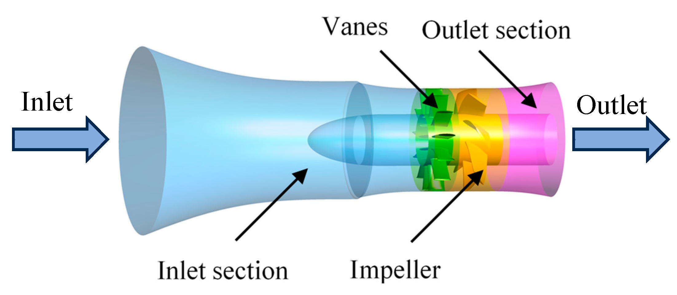
2.1. Axial-Flow Unit

This article conducts research on an axial-flow unit. The axial-flow unit consists of four components: the inlet section, guide vane, impeller, and outlet section. The upstream guide vane plays a guiding role in ensuring uniform flow in the inlet section. The impeller is the core component of the unit, used to convert rotating mechanical energy into water kinetic energy. The rotational speed of the impeller is 260 r/min. The guide vanes consist of thirteen blades, while the impeller is equipped with seven blades. The blade tip of the impeller is not touching the casing; there is a gap between them. Under design (not worn machinery) conditions, the impeller is non-eccentric, and the clearance width h_tc is 3.3 mm. The schematic diagram of the fluid domain of the axial-flow unit under design conditions is plotted in Figure 1; its parameters are listed in

Table 1. Parameters of axial-flow unit.

Parameter	Notation	Value
Rotation speed (r/min)	n	260
Impeller tip diameter (m)	Dtip	1.058
Tip clearance width (mm)	htc	3.30
Impeller blade number	Ni	7
Vane blade number	Nv	13
Rated flow rate (m3/s)	Qr	7095
Rated head	Hr	2.39
Rated efficiency	ηr	0.758

.

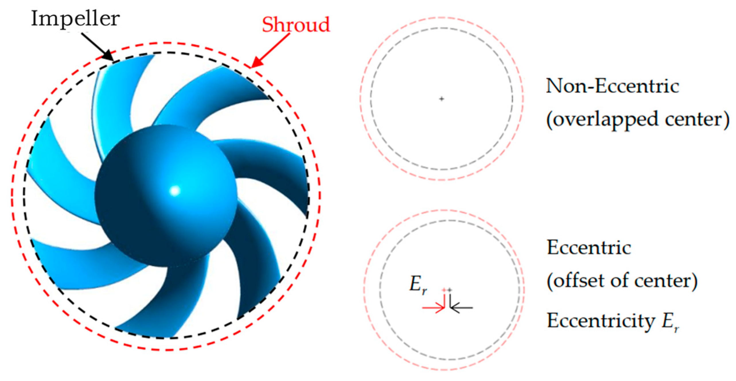
2.2. Impeller Eccentricity

This article mainly analyzes the impact of the eccentricity of the impeller on the performance of the unit, impeller radial force, and pressure pulsation. The definition of the eccentricity of the impeller is shown in Figure 2. As shown in the figure, the impeller and casing are both circular. Under design conditions, the impeller is non-eccentric, and the impeller center and casing center overlap each other. Under eccentric conditions, a certain difference between the impeller center and the casing center exists. This article defines the linear distance between the two centers as the eccentricity of the impeller E_r. It mainly considers two situations: design condition and eccentric condition. Under design (new machinery) conditions, the impeller is not eccentric, and the width of the blade tip gap is 3.3 mm. Under eccentric conditions, the eccentricity E_r value is 1.65 mm. This eccentricity is very tiny against impeller size, as the ratio of eccentricity to the tip diameter D_tip of the impeller is only 0.16%, which is almost imperceptible in actual production.

3. Numerical and Mathematical Methods

3.1. Detached Eddy Simulation Model

To balance computation accuracy and resource cost, this study selected Detached Eddy Simulation (DES) [30] for modeling. DES is a turbulence model proposed by Strelets et al., which combines Reynolds-Averaged Navier–Stokes (RANS) [31] and large eddy simulation (LES) [32] to reduce calculation resources and ensure accuracy. Its basic idea is to use the RANS method in the flow attachment region characterized by dissipation, while the LES method is used to calculate flow turbulence in the separation region characterized by large eddy transport. The DES turbulence model combines the advantages of the LES method in accurately simulating turbulent flow and retaining detailed flow field details while overcoming the large amount of calculation needed for the near wall area. It is a turbulence model widely used in the research of impeller clearance flow based on computational fluid dynamics. The continuity equation and momentum equation in the RANS equation are shown as follows:

$${\displaystyle \frac{\partial \overline{u}}{\partial x_i}}=0$$

(1)

$${\displaystyle \frac{\partial \left(p{\overline{u}}_i\right)}{\partial t}}+\rho {\displaystyle \frac{\partial \left({\overline{u}}_i{\overline{u}}_j\right)}{\partial x_j}}=-{\displaystyle \frac{\partial p}{\partial x_j}}+\mu {\displaystyle \frac{\partial }{\partial x_j}}\left({\displaystyle \frac{\partial {\overline{u}}_i}{\partial x_j}}+{\displaystyle \frac{\partial {\overline{u}}_j}{\partial x_i}}\right)-\rho {\displaystyle \frac{\partial \left(\overline{{u^{\prime }}_i{u^{\prime }}_j}\right)}{\partial x_j}}$$

(2)

In the DES method, the calculation formula for the resolution scale l_DES of RANS and LES is [33]:

$$l_{DES}=\min \left\{l_{RANS},l_{LES}\right\}$$

(3)

$$l_{RANS}=k^{1/2}/\left({\beta }^{*}\omega \right)$$

(4)

$$l_{LES}=C_{DES}\mathsf{\Delta }$$

(5)

$$\mathsf{\Delta }=\min \{\mathsf{\Delta }x,\mathsf{\Delta }y,\mathsf{\Delta }z\}$$

(6)

In the formula, ${\beta }^{*}$ is the SST model constant, coefficient C_DES = 0.65, and Δ is the grid scale.

3.2. Variational Mode Decomposition

Variational Mode Decomposition (VMD) [34] is an adaptive and completely non-recursive signal decomposition method based on Empirical Mode Decomposition (EMD) [35]. It can achieve adaptive segmentation of various components in the frequency domain of the signal, effectively avoiding the problem of modal aliasing in EMD [36]. Variational mode decomposition decomposes the original signal by constructing and solving variational problems. VMD assumes every signal can be decomposed to intrinsic mode functions (IMFs), and the number is defined as k, with center frequency and limited bandwidth. The sum of the estimated bandwidth of each IMF component is minimized, and the sum of these k mode functions is equal to the original signal as a conditional construction variational problem [37]. Finally, by iteratively searching for the optimal solution of the variational model, the center frequency and bandwidth of each component are determined. This method can adaptively achieve frequency domain decomposition of non-stationary nonlinear signals and effective separation of various components, avoiding the occurrence of modal aliasing [36], and has good robustness and adaptability. At present, the VMD method has shown great application value in mechanical fault detection, giving a theoretical basement to apply VMD for analyzing pressure pulsation under eccentric working conditions.

4. Computational Fluid Dynamics Settings

4.1. Setup of Simulation

In this study, the flow inside the axial-flow unit was simulated using the commercial software ANSYS CFX 12, and the DES turbulence model was selected as the turbulence model. The study employs water as the working medium at a temperature of 25 °C, possessing a density of ρ = 10³ kg/m³ and a kinematic viscosity of ν = 10⁻⁶ m²/s. The reference pressure is the standard atmospheric pressure. The following boundary conditions are applied:

(1)

The inflow of the inlet section is set as the computational domain inlet boundary; the condition is set as the velocity inlet type. Inlet conditions include V_in = 2.378 m/s and ∂p/∂x = 0. Additionally, turbulence intensity is 5%.

(2)

The outlet of the exit section is designated as the final computational domain, and the condition of the outlet is set as a pressure outlet. The equation for outlet conditions is p = 1 atm and ∂V/∂x = 0.

(3)

To exchange data among domain parts, several interfaces are adopted. The interfaces between the impeller and guide vane and between the impeller and outlet section are set as rotor–stator interfaces, while the other interfaces are set as stationary. Walls are set as no-slip type.

The maximum iteration number is set to 1 × 10³ in steady simulation. The convergence criteria are the residuals of continuity and momentum equation of 1 × 10⁻⁶. In transient simulation, a total of 20 impeller rotations were considered. Every revolution of the impeller corresponds to 180 time steps, with a maximum iteration limit of 10 iterations per step.

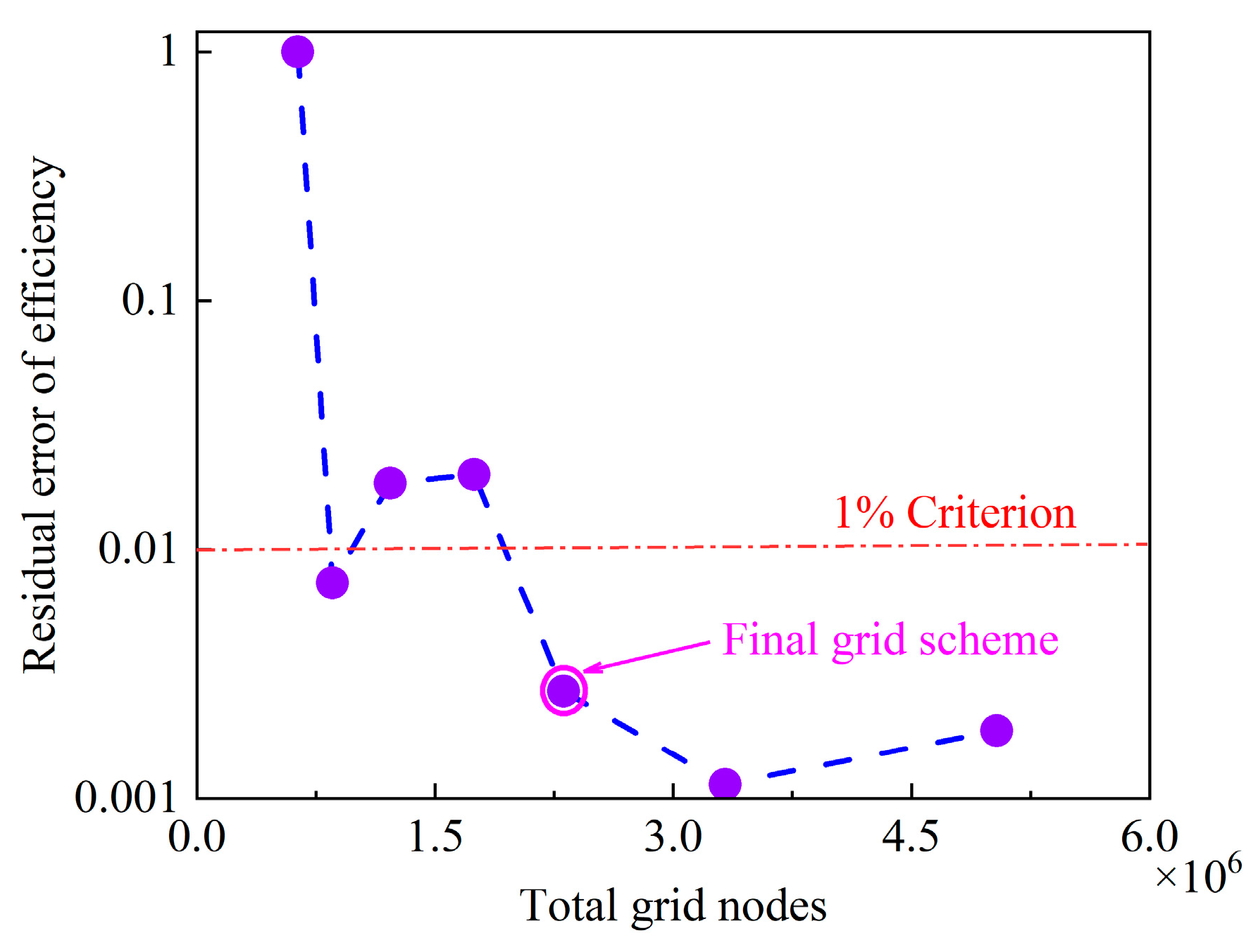
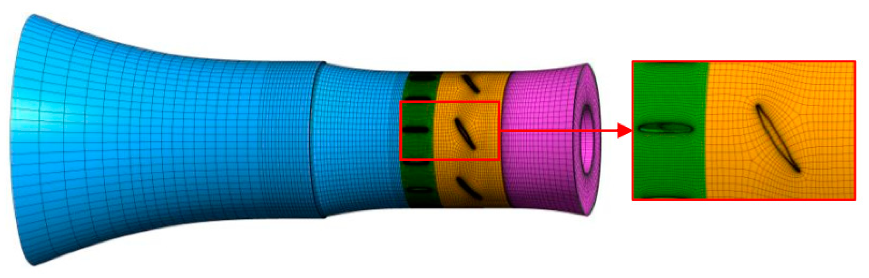
4.2. Grid Preparation and Check

Meshing is the committed step of computational fluid dynamics (CFD). Meshing has an important impact on the accuracy and speed of numerical simulation results. The commonly used grid generation methods are based on structured grid and unstructured grid solutions [38]. Given the benefits of excellent grid quality as enhanced calculation precision and reduced element count, the choice is made to employ a hexahedral structured grid for domain discretization. In this study, the residual efficiency error serves as the metric for grid number assessment. Grid independence evaluations are performed using various grid schemes, with a residual efficiency error below 1% as the benchmark criterion. Figure 3 schematically represents the grid independence assessment. From the figure, it can be seen that when the total grid node count exceeds 2.3 × 10⁶, the remaining error remains less than 1%. A scheme with 2.3 × 10⁶ grid nodes was selected for grid division to balance accuracy and cost; the grid with its parts in different colors is shown in Figure 4 and

Table 2. Mesh node number.

Component	Mesh Node Number
Inlet section	250,760
Vanes	985,906
Impeller	919,472
Outlet section	173,600
Total	2,329,738

. For a better adaptability of the DES model, the y+ value near wall is controlled to smaller than 3, which is an empirically good solution.

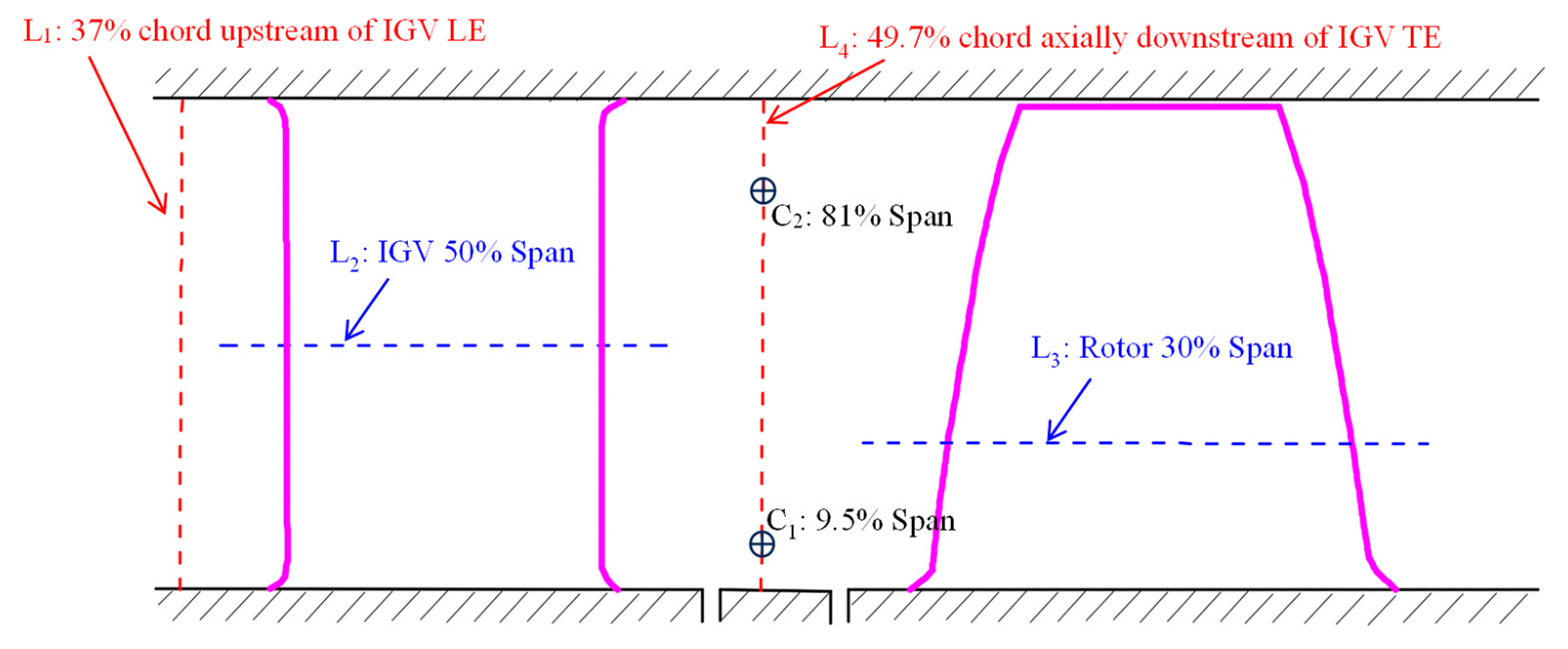
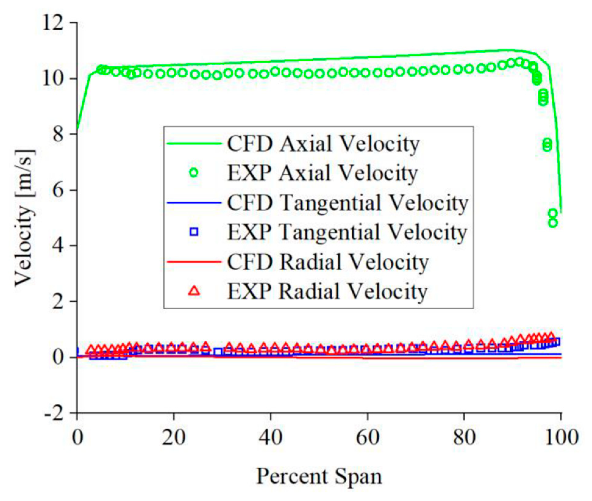
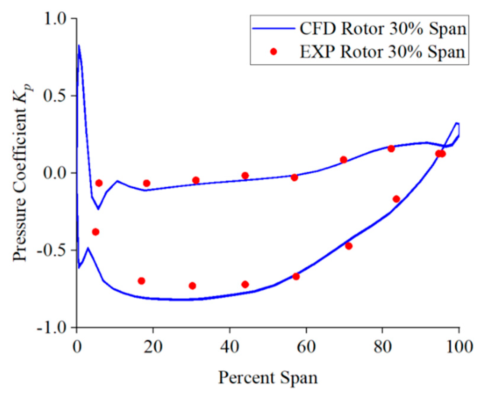
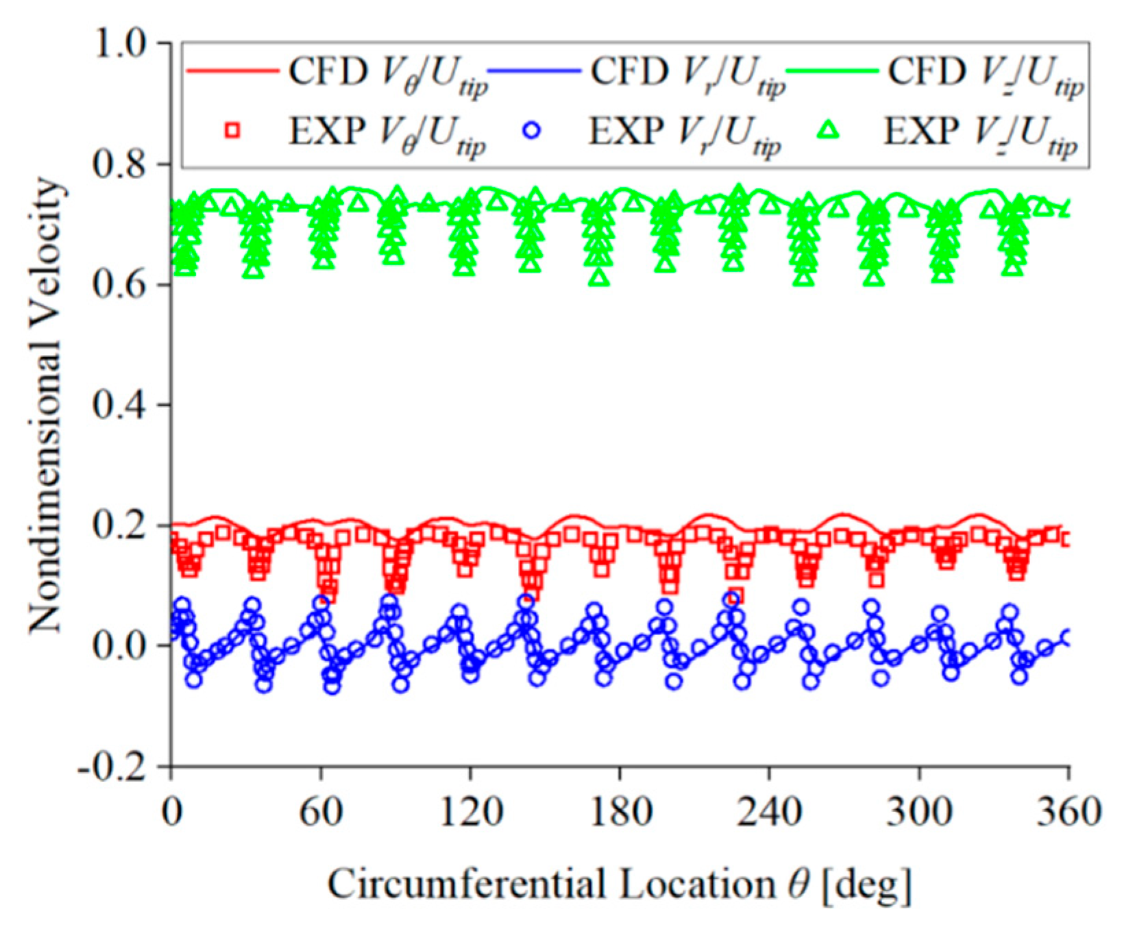
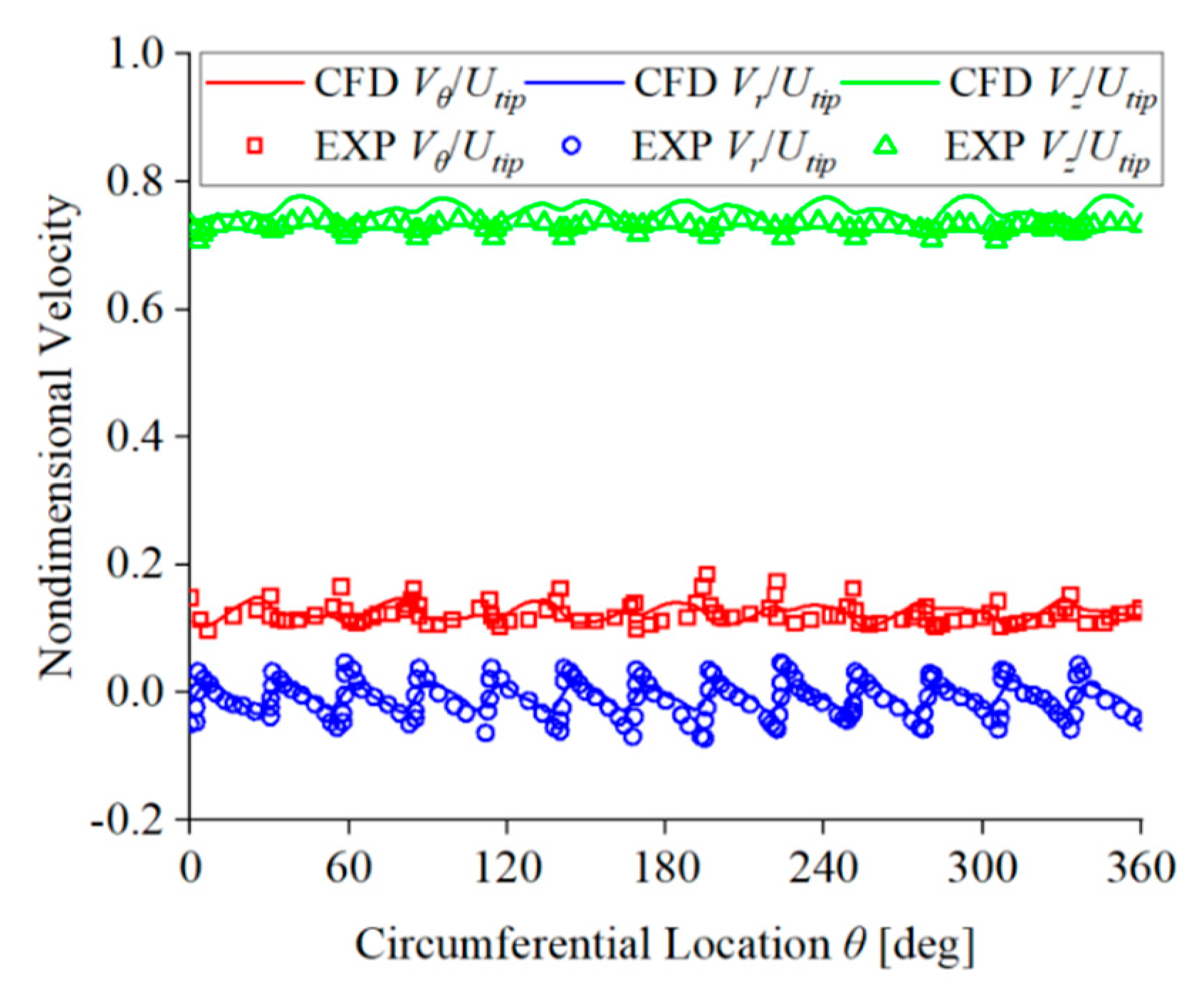
4.3. Experimental–Numerical Validation

This article mainly adopts the method of numerical simulation for research. In order to validate the accuracy of the numerical simulation, a comparison was conducted between the outcomes of the numerical simulation and the experimental results under design conditions. The experimental results were obtained from reference [39]. Figure 5 is a schematic diagram of each measurement position. L₁ and L₄ are two straight lines, with L₁ located at 37% chord upstream of the leading edge (LE) of the inlet guide vane (IGV) and L₄ located at 49.7% chord downstream of the trailing edge (TE) of the inlet guide vane. L₂ and L₃ are the cross-sections of the guide vanes and impeller blades, with L₂ located at 50% span of the IGV and L₃ at 30% span of the impeller blades. C₁ and C₂ are two circles, with C₁ located at the 9.5% wingspan circumference on L₄ and C₂ located at the 81% wingspan circumference on L₄. Subsequently, we compare the velocity and pressure outcomes from both experimental and numerical simulations at different measurement positions.

Figure 6 compares the results from the numerical simulation and experiment of the velocity on monitoring line L₁. The figure clearly illustrates the velocity components in different directions on the monitoring line L₁ obtained by numerical simulation are very close to the experimental results. The axial velocity on the monitoring line L₁ is about 10 m/s, and the tangential velocity and radial velocity fall within 0.1~0.5 m/s.

In order to be consistent with the experimental results, we used another definition of pressure coefficient K_p to quantitatively represent the pressure on the monitoring line in the comparative analysis of experimental data and numerical simulation. The calculation formula for the pressure coefficient K_p is [39]:

$$K_p={\displaystyle \frac{p-p_{\infty }}{\frac{1}{2}\rho U_{tip}^2}}$$

(7)

where p denotes the pressure at different points along the monitoring line, p_∞ denotes the reference pressure at the inlet, and U_tip represents the velocity at the impeller blade’s tip. Under design conditions, the impeller blades rotate at a rotation speed of 260 r/min, while U_tip = 14.5 m/s. Figure 7 illustrates the contrast between the pressure coefficient K_p outcomes from numerical simulations and experimental data on monitoring line L₂. Figure 8 illustrates the contrast between the pressure coefficient K_p outcomes from numerical simulations and experimental data on monitoring line L₃. From the figure, it is evident that the pressure on monitoring lines L₂ and L₃ obtained from numerical simulation is basically consistent with the experimental results. The pressure coefficient of the blade pressure surface on monitoring line L₂ is around 0, and the K_p of the suction surface is approximately −0.3. On monitoring line L₃, the pressure coefficients of the blade’s pressure and suction surface gradually increase. In addition, the numerical simulation results reveal that the pressure at the leading edge of the guide vanes and impeller blades is relatively high, which is due to the heightened localized pressure induced by the fluid impact on the leading edge of the blades. Overall, numerical simulation has the capability to precisely forecast the pressure distribution on the blade surface, supplying a theoretical foundation for subsequent analysis.

Figure 9 compares dimensionless velocity between the numerical simulation and experimental results on monitoring line C₁. Figure 10 compares dimensionless velocity between the numerical simulation and experimental results on monitoring line C₂. In these figures, V_r represents the circumferential velocity of the fluid, V_r represents the radial velocity of the fluid, and V_z represents the axial velocity of the fluid. From these figures, it can be seen that the dimensionless velocities on the monitoring lines C₁ and C₂ obtained from numerical simulation have the same fluctuation period and trend along the circumference as the experimental results, and the data are in good agreement. The range of velocity component fluctuation remains fairly constant at different positions. The preceding analysis demonstrates the accurate capability of numerical simulation in simulating velocity distribution within the impeller channel, and it is effective in analyzing the flow in the unit according to the numerical simulation results.

5. Analysis of Simulation Results

5.1. Performance Comparison

To comprehend the impeller eccentricity influence on the unit performance, we compared the efficiency, power, and head of the unit under design conditions and eccentric conditions, as illustrated in Figure 11. From the figure, it is evident that under design conditions, the efficiency of the unit is about 80%, the power is about 251 kW, and the head is about 2.85 m. The impeller’s eccentricity has minimal effect on the unit’s performance, and compared to the reference operation with no eccentricity (design) conditions, the changes in efficiency, power, and head of the unit caused by eccentricity are less than 1%. It is clear that the impeller eccentricity does not affect the unit’s efficiency. However, it is necessary to explore whether the eccentricity of the impeller causes drawbacks and related hazards, such as vibration, noise, and cavitation, which may affect the unit’s safe operation.

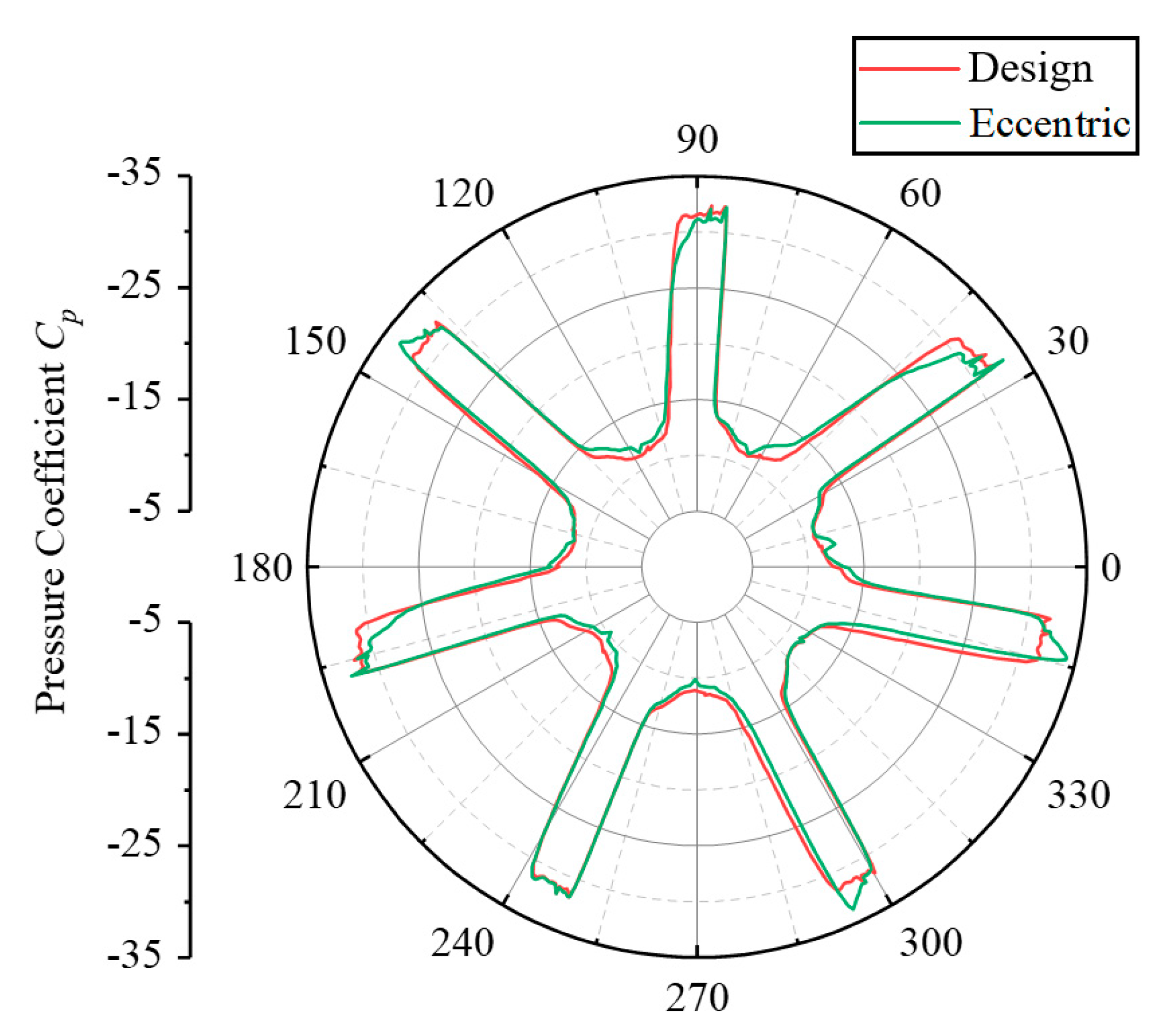
5.2. Comparison of Radial Force

Figure 12 displays the time domain plot of the radial force F_r of the impeller under two operating conditions during three impeller rotation cycles. From the figure, it can be observed that in both cases, the period of radial force pulsation is the same, the waveform is basically stable, and the amplitude (peak-peak value) change is small. The average of radial force and its amplitude of pulsation at eccentric conditions are significantly greater than those under design conditions. Figure 13 shows the average intensity value of radial force and its amplitude comparison on the impeller at two conditions. It illustrates the impeller eccentricity will cause a pronounced rise in the mean impeller radial force intensity, which poses a significant threat to the unit’s safe operation. Under design conditions, the mean radial force intensity of the impeller is 31.38 N, while under eccentric conditions, the mean radial force intensity of the impeller has increased by nine times, reaching 316.30 N. From the comparison of amplitude, it is evident that that the amplitude of the impeller under design conditions is 30.05 N, and the amplitude of F_r under eccentric conditions has increased by about one time, reaching 61.49 N.

The increase in radial force caused by eccentricity is closely linked to the uneven distribution of clearance pressure caused by uneven clearance. In order to quantify the pressure change at the tip clearance of the impeller, in this analysis, a reference line is set at the tip clearance of the impeller, as depicted in Figure 14, and uses the dimensionless pressure coefficient C_p to represent the change in pressure on the reference line. The calculation formula for C_p is as follows (it is distinguished from K_p, which is used to compare experimental data) [40]:

$$C_p={\displaystyle \frac{2\left(p-p_{in}\right)}{\rho V_{in}^2}}$$

(8)

where p is the pressure at various points along the reference line. p_in refers to the mean pressure at the inlet, while V_in refers to the average velocity at the same location. Figure 15 shows the changes in the pressure coefficient on the reference line under two conditions. It is evident from the figure that the pressure coefficient C_p on the reference line is between −5 and −35, and the pressure coefficient is less than zero. This indicates that the pressure at the tip clearance is lower than the average pressure at the inlet of the fluid domain, and cavitation and erosion are prone to occur at the tip clearance. Because of the effect of the impeller blades, the gap pressure distribution exhibits seven distinct cycles along the circumference. Under design conditions, the gap pressure distribution is basically the same across seven cycles. Under eccentric conditions, affected by uneven clearance, some blade passages have a higher pressure, while others have an opposite pressure, which results in certain differences in the distribution of clearance pressure in different blade passages. The uneven distribution of clearance pressure leads to a significant rise in the impeller’s radial force. In addition, the difference in pressure distribution between design and eccentric cases is mainly reflected in the variation of minimum pressure in the circumferential orientation, while the difference in maximum pressure in the circumferential orientation is not obvious.

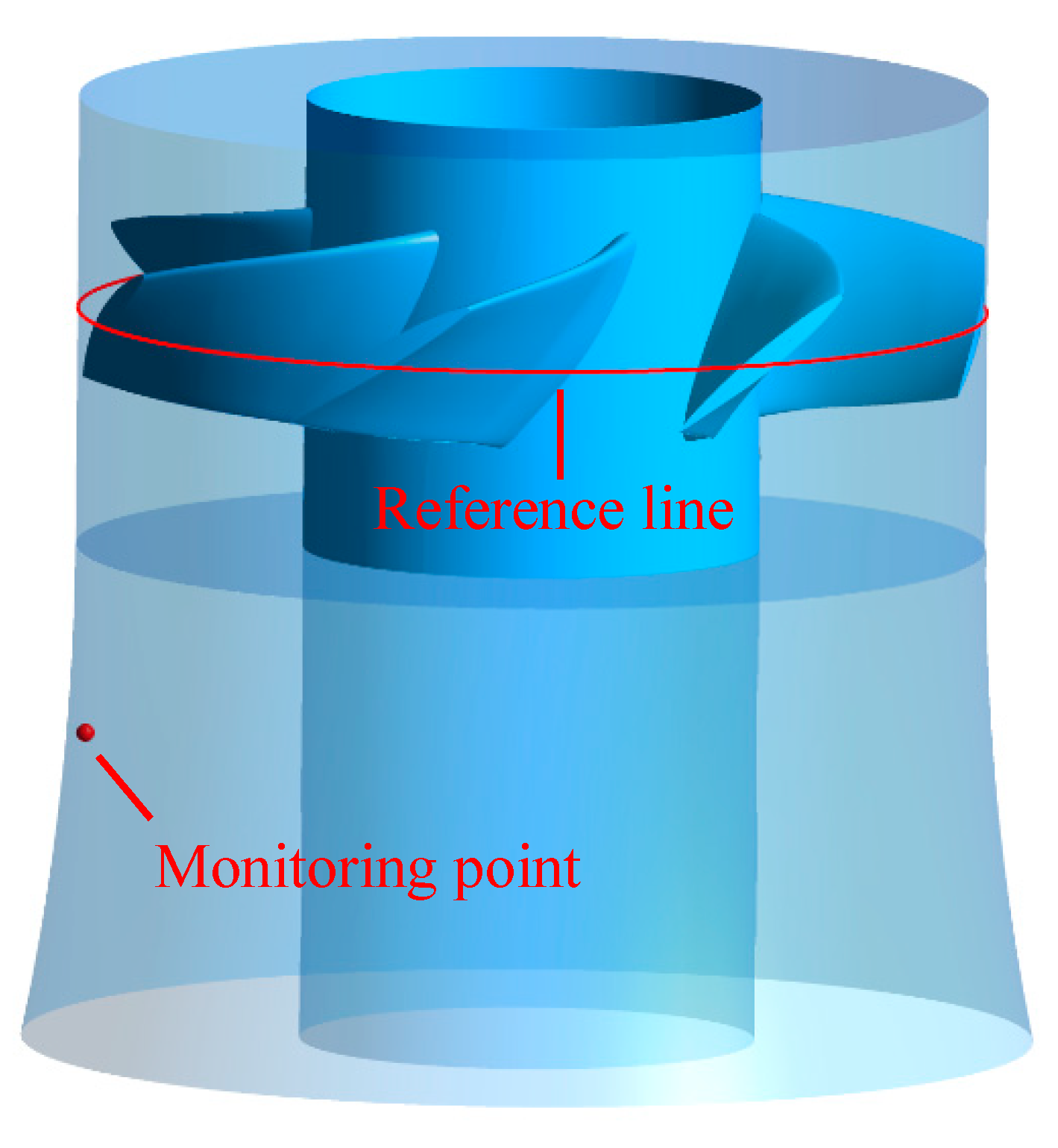
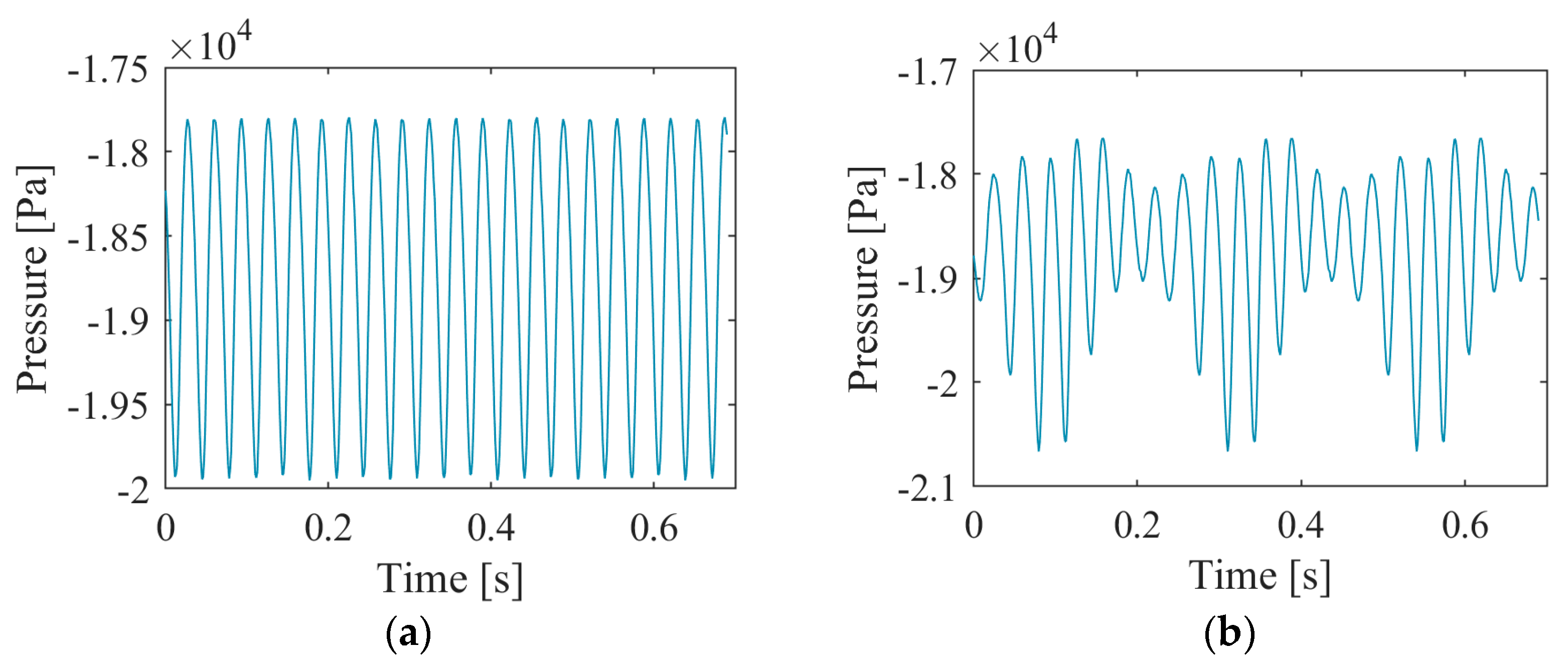
5.3. Pressure Pulsation Comparison

Figure 16 illustrates the time domain diagram of pressure pulsation at the monitoring point during three rotating cycles of the impeller under two conditions, and the location of the monitoring point is shown in Figure 14. From the figure, it can be seen that under different conditions, there are seven peaks and valleys in the time domain of pressure pulsation within an impeller rotation cycle, which is the same as the blade count. This is attributed to the impact of blades on flow during impeller rotation. Under design conditions, each blade has the same impact on flow, and the seven peaks and valleys within a rotating cycle of the impeller are basically the same. Under eccentric conditions, the width of the blade tip gap will change, causing differences in the impact of each blade on flow during a rotation cycle of the impeller, resulting in changes in pressure pulsation at the monitoring point. During a rotating cycle of the impeller, the eccentricity of the impeller will cause an increase in the amplitude of pressure pulsation at the monitoring point, while the average value of pressure pulsation remains basically unchanged.

To further analyze the impact of impeller eccentricity on the pulsation of pressure at the monitoring point, VMD is adopted to decompose the pulsation signals of pressure under different conditions and to obtain the time and frequency domain diagrams of each component, as shown in Figure 17. Here, the original signal is decomposed into five IMFs. The center frequency value gradually increases from IMF5 to IMF1. Among the five IMFs obtained by the VMD method, the frequency of IMF5 is the lowest. Under eccentric conditions, two peaks of frequency can be found. The corresponding values of the peaks are 4.33 Hz and 8.67 Hz, respectively, which are the impeller frequency f_r and 2f_r. There are only three peaks and valleys in the time domain diagram of this mode, which are the same as the rotation period of the impeller. This shows that the IMF5 component is mainly influenced by impeller frequency. Under design conditions, the amplitude of the frequency domain and time domain plots of the IMF5 component is basically zero, indicating that when the impeller is not eccentric, the pressure pulsation at the monitoring point is basically not affected by the impeller frequency.

IMF3 has the highest peak value among all components, with a peak frequency of 30.33 Hz, which is seven times the impeller frequency f_r and is the same as the impeller blade passing frequency f_b. This component is mainly generated due to the influence of blade passage frequency. IMF2 and IMF4 are located on both sides of IMF3, respectively. Under eccentric conditions, the peak frequency of IMF2 is eight times f_r, and the peak frequency value of IMF4 is six times f_r. The frequency difference between these two components and IMF3 is the impeller frequency f_r, which could be attributed to the mutual influence of impeller frequency and blade passage frequency. Under design conditions, due to the small impact of the impeller frequency f_r on pressure pulsation (IMF5), the amplitudes of the IMF2 and IMF4 components are also small. The time domain diagrams of these two components are similar to those of the IMF5 component, with pressure pulsations on both sides of the time domain diagram, while in the middle part of the time domain, the value of pulsation is basically 0.

The IMF1 component has the highest frequency among all components, with a peak frequency of 60.67 Hz, which is twice the blade passing frequency f_b. Under design conditions, the IMF1 frequency diagram component has only one peak. Under eccentric conditions, the IMF1 component is composed of multiple high-frequency and low-amplitude signals, and the frequency difference between each peak is still the impeller frequency f_r, indicating that this component is jointly affected by f_r and f_b. Furthermore, notable distinctions emerge within the time domain graphs of the IMF1 component between the two conditions. Under design conditions, there are 21 identical periods in the IMF1 time domain, which is seven times the rotation period of the impeller. However, at eccentric conditions, there are only three periods, which are the same as the rotation period of the impeller.

By analyzing the pulsation signal decomposed by VMD, it is found that the influence of impeller eccentricity on pressure fluctuation is mainly reflected in increasing impeller frequency on pressure fluctuation, which is consistent with the research results of Lu et al. [41]. Under design conditions, the dominant influence at the monitoring point is from f_b. At eccentric conditions, the pressure pulsation at the monitoring point is jointly affected by f_r and f_b. Figure 18 compares the corresponding amplitudes of f_r and f_b under two conditions. It is evident from the figure that under design conditions, the corresponding amplitude of f_r is 2.6, while under eccentric conditions, the corresponding amplitude of f_r has increased by more than 100 times, reaching 274.4. Under design conditions, the corresponding amplitude of f_b is 976, while under eccentric conditions, the corresponding amplitude of f_b decreases to 785.9.

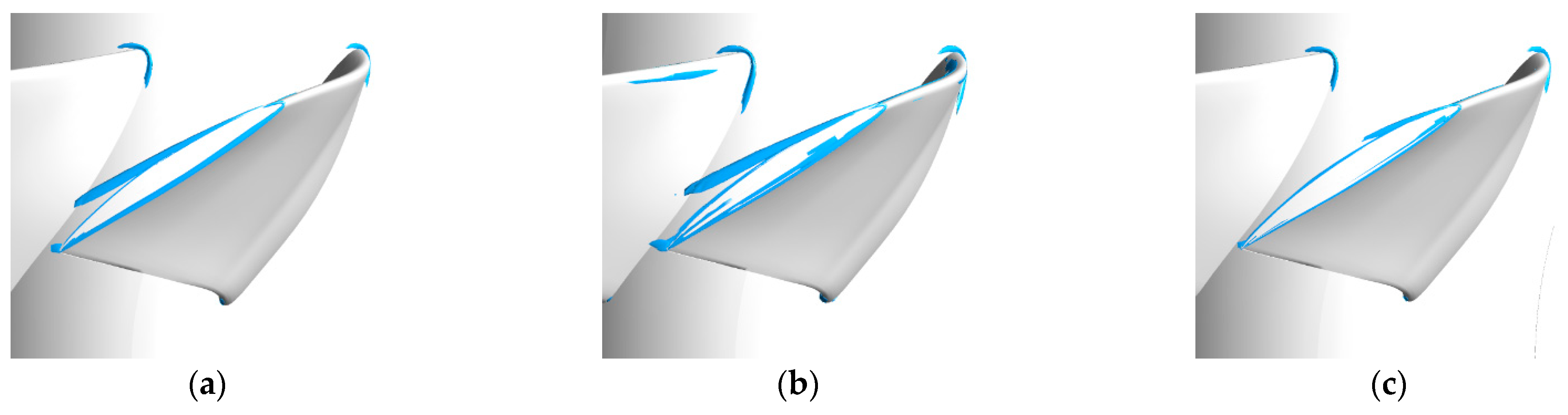
5.4. Comparison of Blade Tip Vortex

Figure 19 illustrates the comparison of the blade tip vortices at different conditions, where the top tip vortices are significantly stronger at the biggest eccentric blade tip than at the non-eccentric blade tip and fill the blade tip edge. At the smallest eccentric blade tip condition, the blade tip vortex is significantly slightly weaker than that at the non-eccentric blade tip condition. In the overall comparison of the three conditions, although the vortex is generated in all three conditions, it is evident, also from the figure, that the vortex is the strongest in the biggest eccentric blade tip condition and the weakest in the smallest eccentric blade tip condition.

6. Conclusions and Discussion

This study compared and analyzed the impact of the eccentricity of the axial-flow impeller on the performance of the unit, as well as on the radial force of the impeller and pressure pulsation. The conclusions are as follows:

(a)

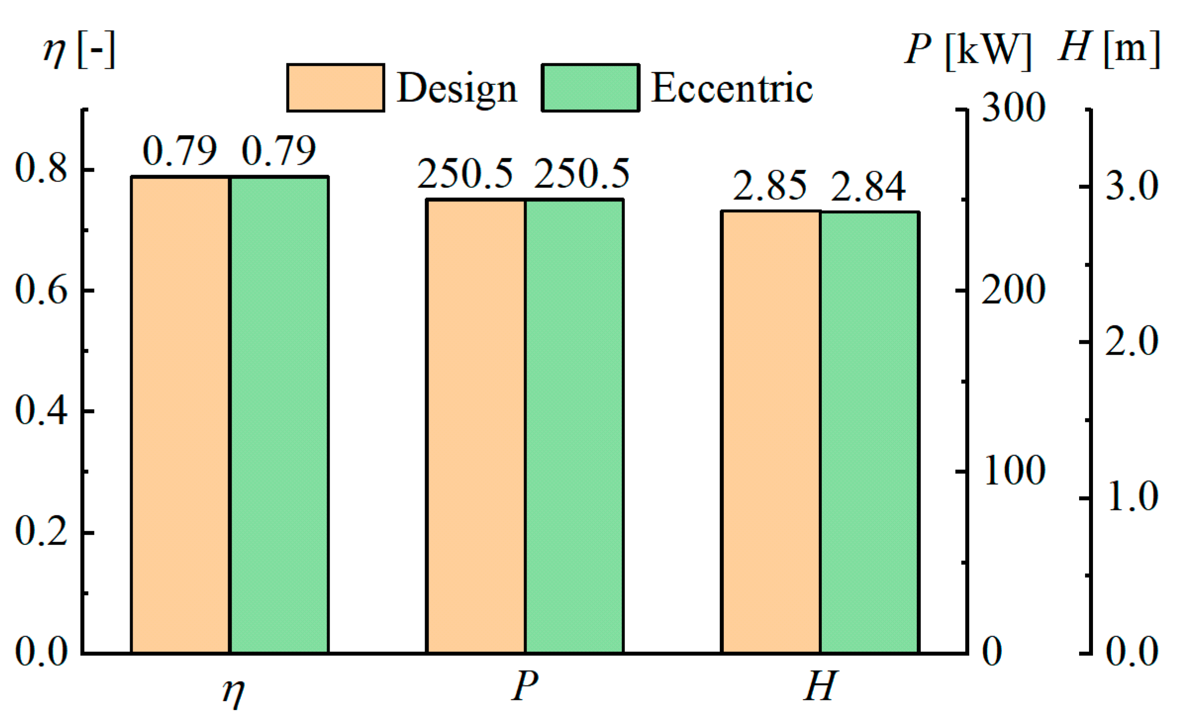
Under eccentric operating conditions, the performance of the unit changes very little. Under design conditions, the efficiency of the unit is about 80%, the power is about 251 kW, and the head is about 2.85 m. When the impeller is eccentric, the efficiency, power, and head of the unit vary by less than 1%.

(b)

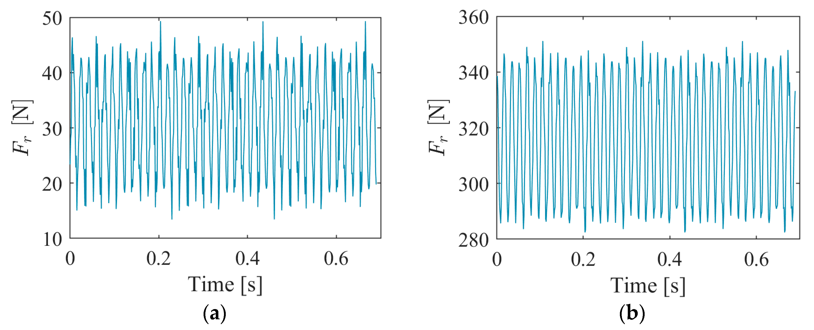
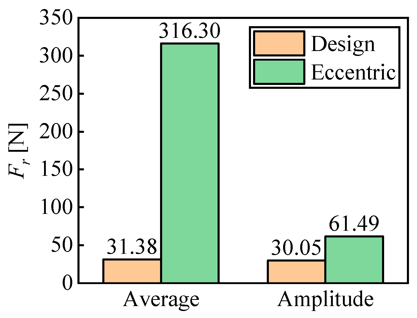
Eccentricity of the impeller can cause a sharp increase in radial force on the impeller. Under design conditions, the average radial force of the impeller is 31.38 N; under eccentric conditions, the average value of the impeller radial force increased by nine times, reaching 316.30 N.

(c)

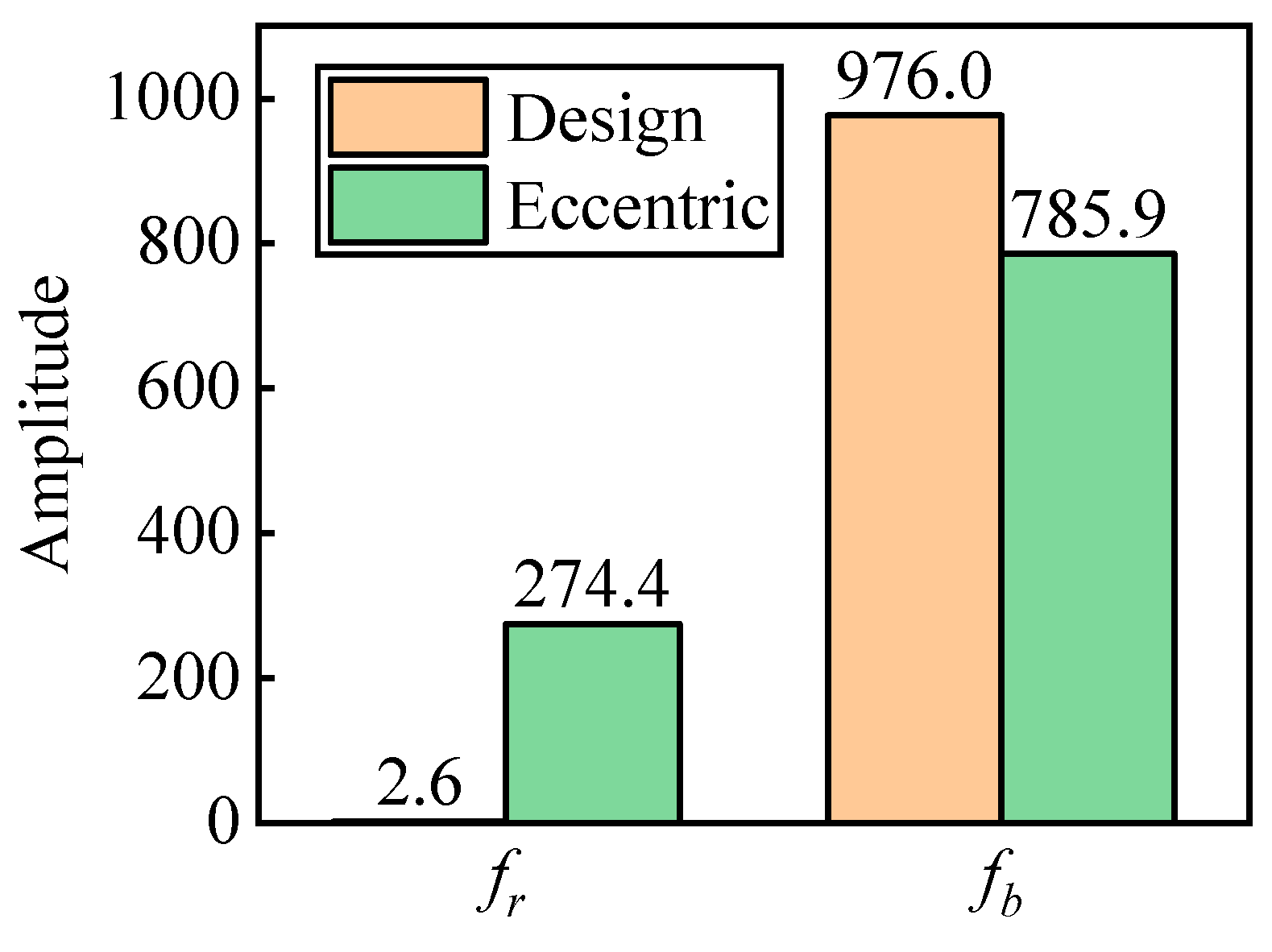
Impeller eccentricity will increase the influence of impeller frequency on downstream pressure pulsation. Under design conditions, f_r has almost no effect on pressure pulsation, with a corresponding amplitude of 2.6. Under eccentric conditions, the amplitude corresponding to f_r increased by more than 100 times, reaching 274.4.

The specific effects of axial-flow impeller eccentricity on unit performance, impeller radial force, and pressure pulsation are clarified in this study, which provides theoretical guidance for the safe and stable operation of axial-flow units. However, the eccentricity of the impeller will inevitably change during the operation of the unit, and different eccentricities will inevitably cause different degrees of impact. In addition, the model simplification existing in numerical simulation will also affect the calculation results, and the subsequent research will focus on the specific analysis of relevant tests.

References

1. Han, H.; Jia, Y.; Zhang, Y. Technology research and test analyses of shaft sealing reactor coolant pump full load test. Large Electr. Mach. Hydraul. Turbine 2017, 251, 21–23. [Google Scholar]
2. Tao, R.; Xiao, R.; Liu, W. Investigation of the flow characteristics in a main nuclear power plant pump with eccentric impeller. Nucl. Eng. Des. 2018, 327, 70–81. [Google Scholar] [CrossRef]
3. Furukawa, A.; Shigemitsu, T.; Watanabe, S. Performance test and flow measurement of contra-rotating axial flow pump. J. Therm. Sci. 2007, 16, 7–13. [Google Scholar] [CrossRef]
4. Miller, G.; Corren, D.; Armstrong, P.; Franceschi, J. A study of an axial-flow turbine for kinetic hydro power generation. Energy 1987, 12, 155–162. [Google Scholar] [CrossRef]
5. Zhang, Y.L.; Li, J.F.; Wang, T.; Xiao, J.J.; Jia, X.Q.; Zhang, L. Pressure distribution on the inner wall of the volute casing of a centrifugal pump. Sci. Technol. Nucl. Install. 2022, 2022, 3563459. [Google Scholar] [CrossRef]
6. Zhu, H.; Bo, G.; Zhou, Y.; Zhang, R.; Cheng, J. Pump selection and performance prediction for the technical innovation of an axial-flow pump station. Math. Probl. Eng. 2018, 2018, 6543109. [Google Scholar] [CrossRef]
7. Al-Obaidi, A.R.; Qubian, A. Effect of outlet impeller diameter on performance prediction of centrifugal pump under single-phase and cavitation flow conditions. Int. J. Nonlinear Sci. Numer. Simul. 2022, 23, 1203–1229. [Google Scholar] [CrossRef]
8. Al-Obaidi, A.R.; Alhamid, J. Investigation of the main flow characteristics mechanism and flow dynamics within an axial flow pump based on different transient load conditions. Iran. J. Sci. Technol. Trans. Mech. Eng. 2023, 47, 1397–1415. [Google Scholar] [CrossRef]
9. Al-Obaidi, A.R. Effect of Different Guide Vane Configurations on Flow Field Investigation and Performances of an Axial Pump Based on CFD Analysis and Vibration Investigation. Exp. Tech. 2023, 48, 69–88. [Google Scholar] [CrossRef]
10. Al-Obaidi, A.R.; Khalaf, H.; Alhamid, J. Investigation of the Influence of Varying Operation Configurations on Flow Behaviors Characteristics and Hydraulic Axial-Flow Pump Performance. In Proceedings of the 4th International Conference on Science Education in The Industrial Revolution 4.0, ICONSEIR, Medan, Indonesia, 24 November 2022. [Google Scholar]
11. Al-Obaidi, A.R. Investigation of effect of pump rotational speed on performance and detection of cavitation within a centrifugal pump using vibration analysis. Heliyon 2019, 5, e01910. [Google Scholar] [CrossRef]
12. Xia, X.; Luo, H.; Li, S.; Wang, F.; Zhou, L.; Wang, Z. Characteristics and factors of mode families of axial turbine runner. Int. J. Mech. Sci. 2023, 251, 108356. [Google Scholar] [CrossRef]
13. Wu, H.; Miorini, R.L.; Katz, J. Measurements of the tip leakage vortex structures and turbulence in the meridional plane of an axial water-jet pump. Exp. Fluids 2011, 50, 989–1003. [Google Scholar] [CrossRef]
14. Zhang, D.; Shi, W.; Bin, C.; Guan, X. Unsteady flow analysis and experimental investigation of axial-flow pump. J. Hydrodyn. Ser. B 2010, 22, 35–43. [Google Scholar] [CrossRef]
15. Lin, F.; Chen, J. Oscillatory tip leakage flows and stability enhancement in axial compressors. Int. J. Rotating Mach. 2018, 2018, 9076472. [Google Scholar] [CrossRef]
16. Wang, J.; Cheng, H.; Xu, S.; Ji, B.; Long, X. Performance of cavitation flow and its induced noise of different jet pump cavitation reactors. Ultrason. Sonochem. 2019, 55, 322–331. [Google Scholar] [CrossRef]
17. Kan, K.; Binama, M.; Chen, H.; Zheng, Y.; Zhou, D.; Su, W.; Muhirwa, A. Pump as turbine cavitation performance for both conventional and reverse operating modes: A review. Renew. Sustain. Energy Rev. 2022, 168, 112786. [Google Scholar] [CrossRef]
18. Sentyabov, A.V.; Timoshevskiy, M.V.; Pervunin, K.S. Gap cavitation in the end clearance of a guide vane of a hydroturbine: Numerical and experimental investigation. J. Eng. Thermophys. 2019, 28, 67–83. [Google Scholar] [CrossRef]
19. Kim, S.; Choi, C.; Kim, J.; Park, J.; Baek, J. Tip clearance effects on cavitation evolution and head breakdown in turbopump inducer. J. Propuls. Power 2013, 29, 1357–1366. [Google Scholar] [CrossRef]
20. Tan, D.; Li, Y.; Wilkes, I.; Vagnoni, E.; Miorini, R.L.; Katz, J. Experimental investigation of the role of large scale cavitating vortical structures in performance breakdown of an axial waterjet pump. J. Fluids Eng. 2015, 137, 111301. [Google Scholar] [CrossRef]
21. Al-Obaidi, A.R. Experimental Diagnostic of Cavitation Flow in the Centrifugal Pump under Various Impeller Speeds Based on Acoustic Analysis Method. Arch. Acoust. 2023, 48, 159–170. [Google Scholar]
22. Zhao, M.; Zhao, W.; Wan, D. Numerical simulations of propeller cavitation flows based on OpenFOAM. J. Hydrodyn. 2020, 32, 1071–1079. [Google Scholar] [CrossRef]
23. Al-Obaidi, A. Experimental and Numerical Investigations on the Cavitation Phenomenon in a Centrifugal Pump. Doctoral Dissertation, University of Huddersfield, Huddersfield, UK, 2018. [Google Scholar]
24. Khalid, M.R.; Reza, K.; Ghorbani, S. Common Failures in Hydraulic Kaplan Turbine Blades and Practical Solutions. Materials 2023, 16, 3303. [Google Scholar] [CrossRef] [PubMed]
25. Posa, A.; Lippolis, A. Effect of working conditions and diffuser setting angle on pressure fluctuations within a centrifugal pump. Int. J. Heat Fluid Flow 2019, 75, 44–60. [Google Scholar] [CrossRef]
26. Li, J.; Zhang, Y.; Liu, K.; Xian, H.; Yu, J. Numerical simulation of hydraulic force on the impeller of reversible pump turbines in generating mode. J. Hydrodyn. Ser B 2017, 29, 603–609. [Google Scholar] [CrossRef]
27. Thomas, H.J. Unstable natural vibration of turbine rotors induced by the clearance flow in glands and blading. Bull l’AIM 1958, 71, 1039–1063. [Google Scholar]
28. Ehrich, F. Rotor whirl forces induced by the tip clearance effect in axial flow compressors. In Proceedings of the International Design Engineering Technical Conferences and Computers and Information in Engineering Conference, Albuquerque, NM, USA, 19–22 September 1993; American Society of Mechanical Engineers: New York, NY, USA, 2021; Volume 6395, pp. 7–17. [Google Scholar]
29. Jung, Y.; Choi, M.; Oh, S.; Baek, J. Effects of a nonuniform tip clearance profile on the performance and flow field in a centrifugal compressor. Int. J. Rotating Mach. 2012, 2012, 340439. [Google Scholar] [CrossRef]
30. Strelets, M. Detached eddy simulation of massively separated flows. In Proceedings of the 39th Aerospace Sciences Meeting and Exhibit, Reno, NV, USA, 8–11 January 2001; p. 879. [Google Scholar]
31. Patankar, S. Numerical Heat Transfer and Fluid Flow; Taylor & Francis: Abingdon, UK, 2018. [Google Scholar]
32. Piomelli, U. Large-eddy simulation-Present state and future perspectives. In Proceedings of the 36th AIAA Aerospace Sciences Meeting and Exhibit, Reno, NV, USA, 12–15 January 1998; p. 534. [Google Scholar]
33. Durbin, P.A. Some recent developments in turbulence closure modeling. Annu. Rev. Fluid Mech. 2018, 50, 77–103. [Google Scholar] [CrossRef]
34. Dragomiretskiy, K.; Zosso, D. Variational mode decomposition. IEEE Trans. Signal Process. 2013, 62, 531–544. [Google Scholar] [CrossRef]
35. Huang, N.E.; Shen, Z.; Long, S.R.; Wu, M.C.; Shih, H.H.; Zheng, Q.; Yen, N.C.; Tung, C.C.; Liu, H.H. The empirical mode decomposition and the Hilbert spectrum for nonlinear and non-stationary time series analysis. Proc. R. Soc. Lond. Ser. A Math. Phys. Eng. Sci. 1998, 454, 903–995. [Google Scholar] [CrossRef]
36. Yan, H.; Bai, H.; Zhan, X.; Wu, Z.; Wen, L.; Jia, X. Combination of VMD Mapping MFCC and LSTM: A New Acoustic Fault Diagnosis Method of Diesel Engine. Sensors 2022, 22, 8325. [Google Scholar] [CrossRef]
37. Xiao, Q.; Li, J.; Sun, J.; Feng, H.; Jin, S. Natural-gas pipeline leak location using variational mode decomposition analysis and cross-time–frequency spectrum. Measurement 2018, 124, 163–172. [Google Scholar] [CrossRef]
38. Kan, K.; Zhang, Q.; Xu, Z.; Zheng, Y.; Gao, Q.; Shen, L. Energy loss mechanism due to tip leakage flow of axial flow pump as turbine under various operating conditions. Energy 2022, 255, 124532. [Google Scholar] [CrossRef]
39. Zierke, W.C.; Straka, W.A.; Taylor, P.D. An experimental investigation of the flow through an axial-flow pump. J. Fluids Eng. 1995, 117, 485–490. [Google Scholar] [CrossRef]
40. Kundu, P.; Sarkar, A.; Nagarajan, V. Improvement of Performance of S1210 Hydrofoil with Vortex Generators and Modified Trailing Edge. Renew. Energy 2019, 142, 643–657. [Google Scholar] [CrossRef]
41. Lu, Z.; Li, N.; Tao, R.; Yao, Z.; Liu, W.; Xiao, R. Influence of eccentric impeller on pressure pulsation of large-scale vaned-voluted centrifugal pump. Proc. Inst. Mech. Eng. Part A J. Power Energy 2023, 237, 591–601. [Google Scholar] [CrossRef]
Figure 1. Fluid domain schematic map.
Water 16 02605 g001
Figure 2. Definition of impeller eccentricity.
Water 16 02605 g002
Figure 3. Grid independence check.
Water 16 02605 g003
Figure 4. Schematic diagram of grid division.
Water 16 02605 g004
Figure 5. Schematic diagram of measurement locations.
Water 16 02605 g005
Figure 6. Comparison between velocity results obtained from numerical simulations and experimental data [40] at L1 position.
Water 16 02605 g006
Figure 7. Pressure coefficient comparison at L2 position.
Water 16 02605 g007
Figure 8. Pressure coefficient comparison at L3 position; experimental data are from ref. [40].
Water 16 02605 g008
Figure 9. Comparison of dimensionless velocity at C1 position; experimental data are from ref. [40].
Water 16 02605 g009
Figure 10. Comparison of dimensionless velocity at C2 position; experimental data are from ref. [40].
Water 16 02605 g010
Figure 11. Comparison of unit performance under different operating conditions.
Water 16 02605 g011
Figure 12. Time domain diagram of the radial force of the impeller. (a) Design condition; (b) eccentric condition.
Water 16 02605 g012
Figure 13. Comparison of radial force intensity and amplitude of the impeller.
Water 16 02605 g013
Figure 14. Reference line and monitoring point.
Water 16 02605 g014
Figure 15. Pressure coefficient distribution on the reference line.
Water 16 02605 g015
Figure 16. Time domain diagram of pressure pulsation at the monitoring point under different conditions. (a) Design condition; (b) eccentric condition.
Water 16 02605 g016
Figure 17. The time domain and corresponding spectrum diagrams of pressure pulsation signals. (a) Design condition; (b) eccentric condition.
Water 16 02605 g017
Figure 18. Corresponding amplitude of characteristic frequency.
Water 16 02605 g018
Figure 19. Comparison of blade tip vortices under different operating conditions. (a) Non-eccentric blade tip; (b) the biggest eccentric blade tip; (c) the smallest eccentric blade tip.
Water 16 02605 g019