Time Series Analysis to Estimate the Volume of Drinking Water Consumption in the City of Meoqui, Chihuahua, Mexico

Abstract

Water is a vital resource for sustaining life and for numerous processes within the transformation industry. It is a finite resource, albeit one that can be renewed, and thus sustainable management is imperative. To achieve this objective, it is necessary to have the appropriate tools to assist with the planning policies for its management. This paper presents a time series analysis approach to measure and predict the pattern of water consumption by humans throughout subsectors (domestic, commercial, public sector, education, industry, and raw water) and total water consumption in Meoqui, Chihuahua, Mexico with data from 2011 to 2023, applying calibration model techniques to measure uncertainty in the forecasting. The municipality of Meoqui encompasses an area of 342 km². The climate is semi-arid, with an average annual rainfall of 272 mm and average temperatures of 26.4 °C in summer and 9.7 °C in winter. The municipal seat, which has a population of 23,140, is supplied with water from ten wells, with an average consumption of 20 ± 579 m³ per user. The consumption of the general population indicates the existence of a seasonal autoregressive integrated moving average (SARIMA) (0,1,2)(0,0,2)₁₂ model. (Sen’s Slope = 682.7, p < 0.001). The domestic sector exhibited the highest overall consumption, with a total volume of 17,169,009 m³ (13 ± 93). A SARIMA (2,1,0)(2,0,0)₁₂ model was estimated, with a Sen’s slope of 221.65 and a p-value of less than 0.001. The second-largest consumer of total water was the “raw water” sector, which consumed 5,124,795 (30,146 ± 35,841) m³ and exhibited an SARIMA (0,1,1)(2,0,0)₁₂ model with no statistically significant trend. The resulting models will facilitate the company’s ability to define water resource management strategies in a sustainable manner, in alignment with projected consumption trends.

1. Introduction

Freshwater is a unique and fundamental element because is a prerequisite for the existence of life. There are no viable alternatives for most of its applications, and yet, despite the fact that it is renewable, it is finite [1]. Moreover, despite its status as a fundamental human right, one in three global inhabitants lack secure access to potable water [2]. Furthermore, there is an inverse correlation between the renewable water supply and population growth. The aforementioned supply has diminished by 58% since 1950, a period during which the global population has tripled, increasing the demand for food. Meanwhile, rising temperatures and the emergence of droughts in regions where they previously did not occur are among the consequences of climate change that affect water availability [3].

The lack of sufficient water resources gives rise to water scarcity, which in turn gives rise to a deficit in water availability for the inhabitants of a defined region [4] Moreover, the scarcity of water results in its predominant allocation for industrial and civil purposes, which in turn precipitates a decline in income and yields from irrigated farmland. This, in turn, has an impact on the replenishment of aquifers, with levels declining by up to 30%. This trend is projected to accelerate in the second half of the century. This has resulted in their depletion and collapse in the 21st century [5], thereby stimulating the development of innovative technologies to improve water management [6]. In this context, the World Health Organization (WHO) has recently estimated that 1.1 billion people lack access to safe drinking water and 2.8 billion lack a minimum level of sanitation. Additionally, at the 2015 United Nations Sustainable Development Summit, one of the “Global Sustainable Development Goals” (SDGs) was related to water, with the objective of ensuring its universal access [7].

The findings of numerous studies, including El Garouani et al. [8], indicate the importance of groundwater level analysis and modeling in evaluating the status of water resources. This will facilitate the prediction of groundwater fluctuations and trends, thereby enabling for the initial stages of effective water management [9]. Conversely, in numerous developing countries, the paucity of financial resources and the low priority accorded to water and sanitation services constrain both the upkeep and expansion of these services. Furthermore, the lack of accountability, corruption, and ineffective management hinder efforts to improve water and sanitation [10].

The Chihuahuan Desert ecosystem, which extends from central Mexico to the southeastern United States, is confronted with significant challenges posed by drought and excessive freshwater withdrawals. These challenges are a consequence of population growth and the conversion of land from natural ecosystems to irrigated landscapes. Projections of climate change in the region indicate an increased likelihood of more frequent and prolonged droughts, alterations in precipitation seasonality, and elevated temperatures. Such changes may result in increased evaporative losses and reduced aquifer recharge [11]. The city of Meoqui is located within this region. A local analysis has been conducted to evaluate the consumption of fresh water. We hypothesized that water consumption has been changing in Meoqui, Chihuahua over the period under analysis. Accordingly, the objective of this study was to develop a statistical model for understanding the utilization of water resources. For this reason, a time series analysis based on past observations was employed, as the ARIMA model—a widely utilized tool for forecasting trends in hydrological data—was used as an appropriate means of anticipating future developments in water resources [9].

2. Materials and Methods

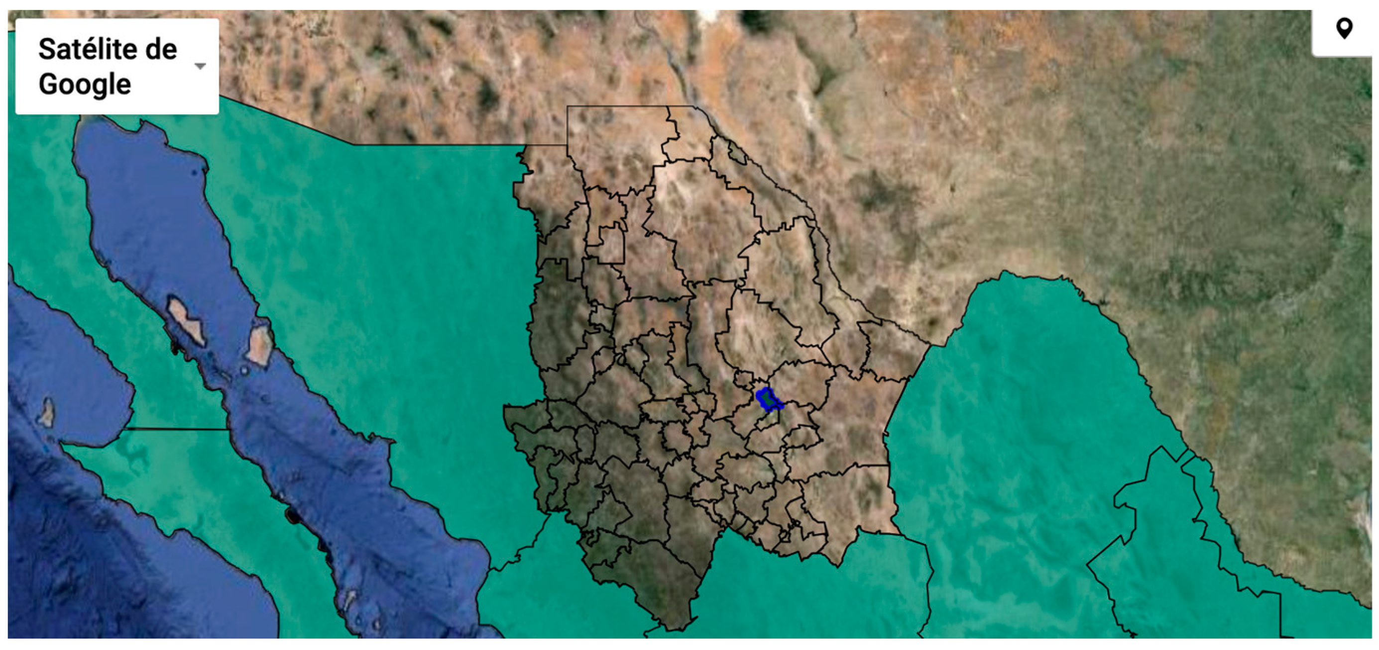
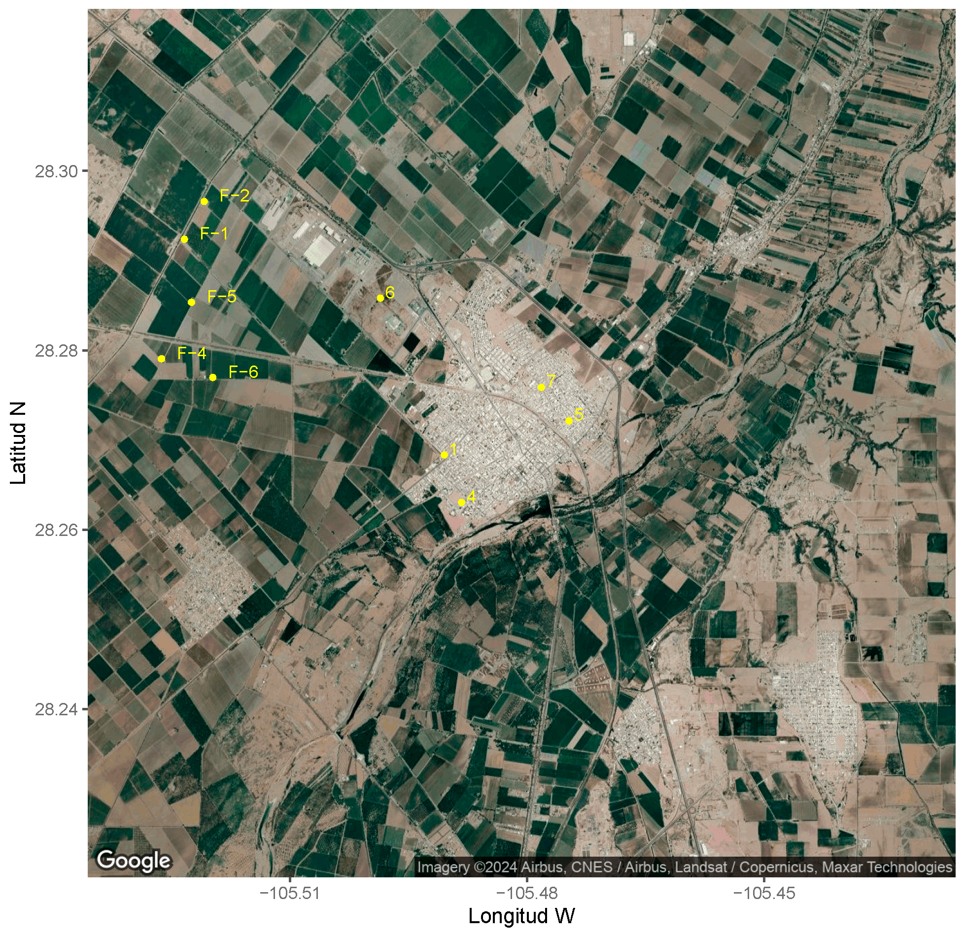
2.1. Research Site

The research site was located within the municipality of Meoqui, within the state of Chihuahua, Mexico. The geographical coordinates of the site were 28°16′0″ N, 105°28′56″ W. The municipal seat is Ciudad de Meoqui, situated on the left bank of the San Pedro River (Figure 1).

The topography of the Meoqui region is predominantly flat, with an average altitude of 1200 m above sea level. The region is distinguished by the presence of extensive plains situated on the banks of the San Pedro River.

The area is situated within the physiographic province of mountains and basins, which is distinguished by its extensive, flat valleys that are elongated and oriented northwest–southeast. The valleys are separated by high and narrow mountain ranges that run parallel to them and are limited by fault scarps. The mountain ranges within the municipality exhibit a range of elevations, reaching up to 300 m above the valley level. The municipality of Meoqui is home to two notable mountain ranges, the Ojuelos Sierra and the Salgadeños Hills. The Ojuelos Sierra reaches an altitude of 1520 m, while the Salgadeños Hills reach 1470 m.

The region is located between the Gulf basin and is home to two major rivers, the San Pedro and the Conchos, which provide invaluable irrigation resources for agricultural activities, thereby contributing to the region’s economic stability.

The climate is classified as semi-arid, with precipitation levels falling below the threshold for aridity but above the threshold for hyperaridity. The temperature demonstrates a range of variation, with a minimum of −2 °C in January and a maximum of 13 °C, and a minimum of 38 °C in August and a maximum of 42 °C in June.

The municipality of Meoqui encompasses an area of 370 km² which positions it 66th in terms of territorial extension among the municipalities of the state. This represents 0.149% of the total surface area of the state.

The city of Meoqui is situated within the boundaries of the San Pedro River wetland, a natural area that was designated as a Ramsar Site in 2012. The region is of considerable ecological significance due to its high level of biodiversity and its importance as a habitat for aquatic birds.

The water has gained recognition for its palatability and quality, which is rich in minerals and deemed safe for human consumption. A number of beverage companies have established operations in the vicinity of the San Pedro River, including the multinational Coca-Cola, the local Refrescos Unión, and the Heineken brewery.

The predominant soil type in the central portion of the area is a yermosol habitat, which is medium in texture and occurs on slopes that are either level or broken. These soils are found in association with lithosols and/or regosols eutric, luvisol, which contain inclusions of rendzinas and/or solonetzsortic, and also occur on medium-textured substrates. In the absence of any associations or inclusions, the soil is in a saline phase.

The predominant land use is agriculture, with a significant livestock component. In terms of land tenure, the first category is private property, which encompasses 29,362 ha, representing 58.72% of the total area. The second largest category is that of ejido property, which encompasses 10,903 ha, or 21.78% of the total area, distributed across three ejidos. A total of 846 ha have been designated for urban use.

2.2. Junta Municipal de Aguas y Saneamiento (JMAS) of Meoqui, Chihuahua

JMAS is a decentralized governmental entity within the government of the state of Chihuahua. The objective of the agency is to facilitate the provision of public sector services pertaining to the treatment and distribution of drinking water within the municipality of Meoqui, Chihuahua. The agency commenced operations in 1957 under the name Junta Federal de Agua Potable (Federal Potable Water Board) and are responsible for the maintenance and construction of water and sewer infrastructure for over 14,000 domestic, commercial, and industrial connections throughout the municipality. Of these, 8000 are situated within the municipal capital, while 6700 are in rural areas. The water service is available 24 h a day, with prompt attention to any identified leaks. Furthermore, the primary urban center is equipped with four elevated tanks, which collectively possess a total storage capacity of 1150 m³.

In the municipality, a total of 94,000 m³ of drinking water piping has been installed, in addition to 80,000 m of sanitary sewerage piping in the municipal capital. Annually, approximately 8000 m of sanitary sewer and potable water piping are installed in both municipal and rural areas as a consequence of maintenance and new construction activities.

The city’s wastewater is treated in oxidation ponds situated in the northern and southern regions, representing 33% of the total treatment process. In the final phase of the project, JMAS Meoqui is implementing a plan to construct 30 reverse osmosis plants.

The city has 10 wells where water is extracted. Figure 2 illustrates the geographical positioning of these wells.

2.3. Data Collection

The data was collected from January 2011 to December 2023. Three variables were obtained: Date, type of contract, and consumption. A total of 10,710 users were registered over the course of the study period, with a total of 1,416,952 observations recorded. The following types of contracts (sectors) were derived according to the utilization of the property and, consequently, of the water:

• Domestic: residential dwellings.
• Commercial: comprises businesses engaged in the sale and purchase of goods and services.
• Public: focus is on governmental institutions.
• Education: encompasses schools.
• Industrial: comprises companies engaged in productive business activities, with the exception of those involved in the brewing industry.
• Raw water: companies engaged in the brewing industry.

The consumption data was transmitted by the meters located in the properties by the readers who take readings. This data was stored in a centralized database that also facilitates the generation of water consumption bills and the associated collection of payments.

2.4. Data Analyses

ARIMA models were estimated for each type of sector and in general. The R programming language (Version 4.4.1) [12] and the R-packages broom (Version 1.0.6) [13], dials (Version 1.3.0) [14], dplyr (Version 1.1.4) [15], (Version 1.0.0) [16], ggplot2 (Version 3.5.1) [17], infer (Version 1.0.7) [18], lubridate (Version 1.9.3) [19], modeldata (Version 1.4.0) [20], modeltime (Version 1.3.0) [21], papaja (Version 0.1.2) [22], parsnip (Version 1.2.1) [23], purrr (Version 1.0.2) [24], readr (Version 2.1.5) [25], recipes (Version 1.1.0) [26], reshape2 (Version 1.4.4) [27], rsample (Version 1.2.1) [28], scales (Version 1.3.0) [29], stringr (Version 1.5.1) [30], tibble (Version 3.2.1) [31], tidymodels (Version 1.2.0) [32], tidyr (Version 1.3.1) [33], tidyverse (Version 2.0.0) [32], timetk (Version 2.9.0) [34], tinylabels (Version 0.2.4) [35], trend (Version 1.1.6) [36], tune (Version 1.2.1) [37], workflows (Version 1.1.4) [38], workflowsets (Version 1.1.0) [39], and yardstick (Version 1.3.1) [40] for all our analyses.

The results are presented in two distinct sections. The initial section presents a descriptive account of the data, including measures of central tendency and dispersion. The second section employs a time series analysis, specifically autoregressive integrated moving average (ARIMA) models, as outlined by Box et al. [41]. A variant of the Hyndman–Khandakar algorithm [42] was employed for the purpose of model selection. This algorithm integrates unit root tests, Akaike Information Criterion (AICc) minimization, and maximum likelihood estimation (MLE) to derive an ARIMA model.

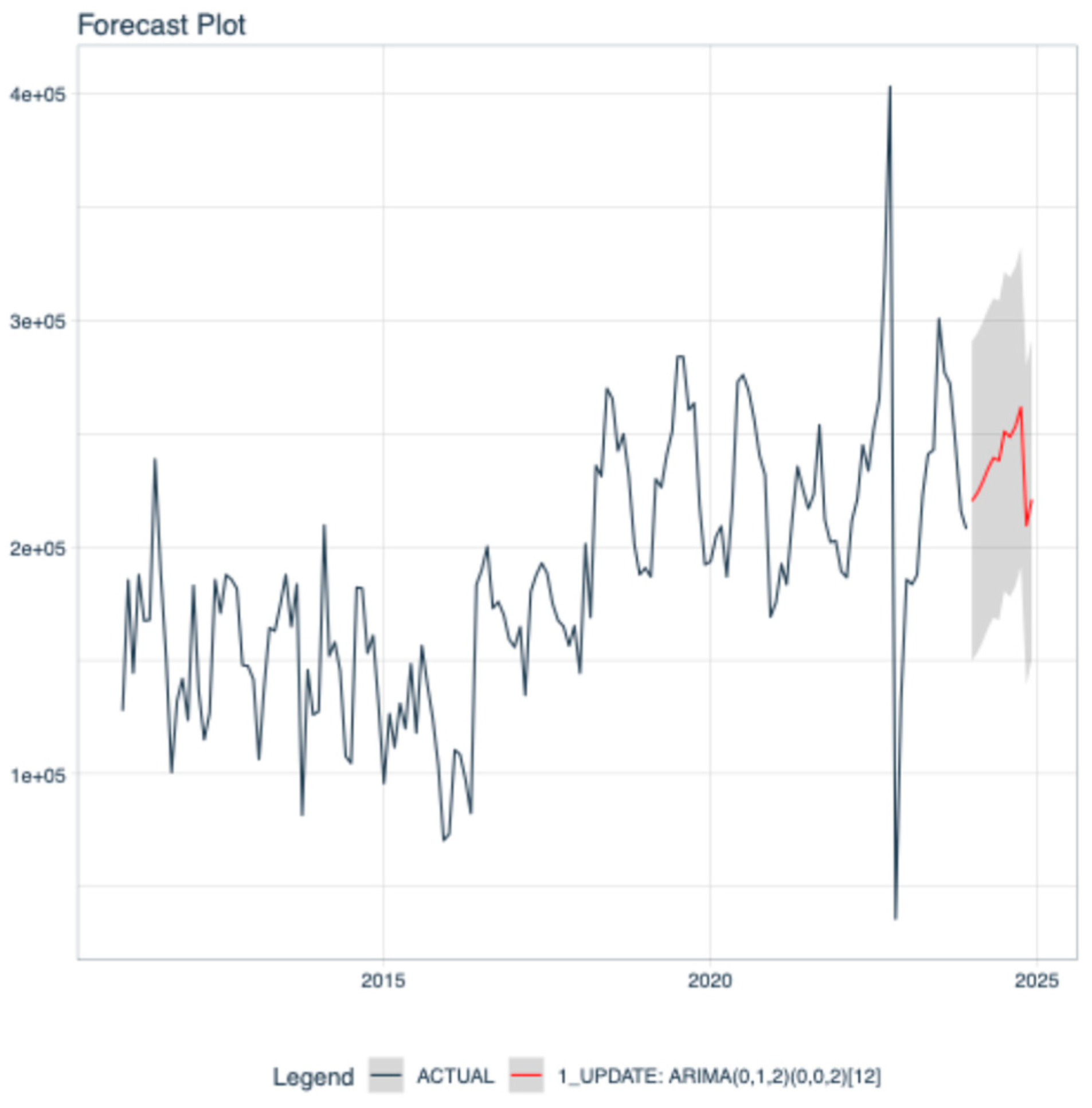
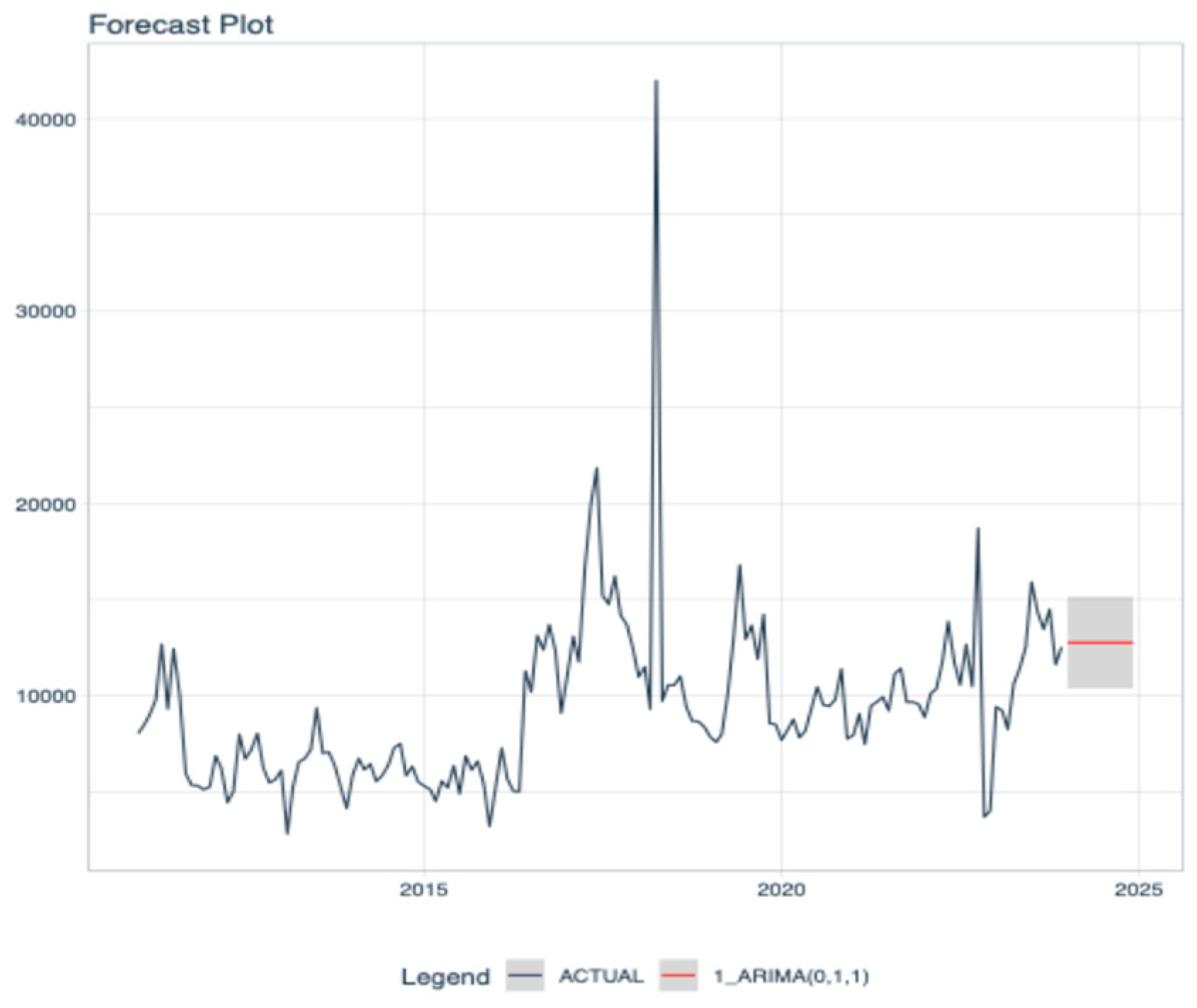
2.5. ARIMA Model Forecast

Box et al. [41], for a given time series, forecasted observation is calculated by the following equation:

$$Y_t=Y_1+Y_2+Y_3+\cdots +Y_t$$

where,

$Y$ is the observations in the time of $t$.

If $P$ is equal to 1

When P > 1, this equation converts into the following:

$$Y_t=c+{\varphi }_1{Y}_{t-1}+{\varphi }_2{Y}_{t-2}+\cdots +{\varphi }_p{Y}_{t-p}+e_t$$

In a study by Patle et al. [43], the two constants $c$ and ${\varphi }_1$ are employed to address the random error in $t$, while $e_t$ is utilized to consider prior errors in a manner analogous to that described by the following equation:

$$Y_t=c+e_t-{\varphi }_1{e}_{t-1}-{\varphi }_2{e}_{t-2}-\cdots -{\varphi }_q{e}_{t-q}$$

2.6. Sen’s Slope Estimator

In general, the slope is employed for the evaluation of straight patterns through the processing of least squares estimation via linear regression. The slope estimation formula, as proposed by Sen [44], is presented in the following equation:

$$Q={\displaystyle \frac{Y_{i^{\prime }}-Y_i}{i^{\prime }-i}}$$

where,

Q is an estimated slope.

$Y_{i^{\prime }}$ is the sum of the values at times $i^{\prime }$ and $i$, where $i^{\prime }$ is greater than $i$.

Sen’s judge of the slope in the middle of N’s ups of Q.

2.7. Mann-Kendall Trend Test

The Mann–Kendall test is a nonparametric method employed for the analysis of trends in time series data [45]. The principal advantage of the Mann–Kendall test is that it does not require the prior specification of a statistical distribution, which is a prerequisite of parametric methods. The null hypothesis ($H_0$) of the Mann–Kendall test is that there is no trend or serial correlation among the population under analysis. In contrast, the alternative hypothesis ($H_1$) postulates the existence of an increasing or decreasing monotonic trend.

$$S=\sum _{i=1}^{n-1}\sum _{j=i+1}^{n}sign\left(x_j-x_i\right)$$

where the Mann–Kendall statistic is S and sign is the signum function. Sign $\left(x_j-x_i\right)$ calculated from:

$$sign\left(x_j-x_i\right)=\left\{\begin{array}{l}+1\mathrm{if}\left(x_j-x_i\right)>0,\\ 0\mathrm{if}\left(x_j-x_i\right)=0,\\ -1\mathrm{if}\left(x_j-x_i\right)<0\end{array}\right.$$

3. Results

3.1. Descriptive Analysis Approach

Total Consumption

JMAS Meoqui, in Chihuahua, Mexico, has assembled a comprehensive data set pertaining to the potable water consumption of a total of 6 types of users or type of contracts. The results demonstrate that the mean extraction of the aggregate of these sectors during the analyzed period was 20 ± 579 m³, and a total of 28,814,778 m³ during the years for which information was available.

Table 1. Measures of central tendency and dispersion for the consumption of water in m³ for each sector in the city of Meoqui, Chihuahua.

	Mean	Sd	Sum
Domestic	13	93	17,169,009
Commercial	16	126	1,460,194
Public	38	108	585,201
Education	95	237	780,562
Industrial	1536	5945	3,695,017
Raw water	30,146	35,841	5,124,795

presents the mean, standard deviation, and total m³ consumption from each sector in Meoqui, Chihuahua. The greatest total quantity of m³ consumption was the domestic sector, with an average of 13 ± 93 m³ and a total of 17,169,009. The next greatest quantity of potable water consumption was raw water, with an average of 30,146 ± 35,841 m³ and a total of 5,124,795 m³.

3.2. Time Series Analysis

The Greek letters utilized for the model estimators are as follows:

tau ($\tau$) is employed for the dependent variable.

phi ($\varphi$) is utilized for the autoregressive component.

eta ($\eta$) is used for the moving averages.

mu ($\mu$) is used for mean.

delta ($\delta$) is used for drift.

epsilon ($ϵ$) for error.

3.2.1. Total Population

A total of 10,710 contracts were subjected to analysis over the specified period. Not all of them were in force during this period, but they were considered since they consumed water. The results of the time series analysis showed the presence of a SARIMA (0,1,2)(1,0,0)₁₂ model. The initial segment of the model indicated that consumption patterns for the general population were not influenced by the preceding month’s consumption (AR = 0 month) and a positive trend was estimated (I = 1) as well as small variability (MA2). With regard to monthly seasonality, a one-month autocorrelation was also estimated, devoid of moving average effects or differencing (Figure 3). Prior to 2016, a notable decline in water consumption was observed, which was attributed to a number of factors. However, there has been a persistent and significant increase in consumption since that time. Furthermore, the model incorporated seasonal variations, with higher consumption observed during the warmer months. The Mann–Kendall trend test, S = 6400, indicated a monotonic increase in general water consumption; Sen’s slope indicated an increase of 682.7 m³ per month [z = 8.7772, n = 168, p-value < 0.001] over the time series. The estimated model is presented in the following Equation (1):

$$\begin{array}{cc}{\tau }_t\hfill & =\left(-0.5920{\eta }_{t-1}-0.2696{\eta }_{t-2}\right){\left(0.3390{\varphi }_{t-1}\right)}_{12}\hfill \\ {ϵ}_t\hfill & \sim NID\left(0,1.47\times {10}^9\right)\hfill \end{array}$$

(1)

3.2.2. Domestic Sector

In the context of the domestic sector, analysis was conducted on the 9780 contracts. The total consumption recorded during the period was 17,169,009, amounting to a volume of 13 m³. The mean was calculated to be 13, with a standard deviation of 93 m³ (Table 1).

A SARIMA (2,1,0)(2,0,0)₁₂ with drift model was estimated from the dataset of this sector. The initial component of the model indicated that consumption patterns were influenced by the preceding two months of consumption (AR = 2 months). In order to achieve stationarity, differencing was an indispensable step in the process. A seasonal component was identified, whereby consumption patterns from the preceding two months exerted an influence (AR2). The observed data and 1 year forecasting values are presented in Figure 4. The data also illustrated a persistent decline in consumption until 2016. Subsequently, an upward trajectory was observed. The graph illustrates a discernible seasonal pattern, which can be attributed to the influence of the cold and hot seasons. The Mann–Kendall trend test = 4238 indicated a monotonic increase in monthly water consumption and the value of Sen’s slope showed an increment of 221.65 m³ per month by this sector [z = 5.8117, n = 168, p-value < 0.001] over the time series model. The Equation (2) estimated model is as follows:

$$\begin{array}{cc}{\tau }_t\hfill & =\left(-0.3002{\varphi }_{t-1}-0.2893{\varphi }_{t-2}\right){\left(0.1863{\varphi }_{t-1}+0.1747{\varphi }_{t-2}\right)}_{12}+\delta 309.435\hfill \\ {ϵ}_t\hfill & \sim NID\left(0,\mathrm{591,688,785}\right)\hfill \end{array}$$

(2)

3.2.3. Commercial Sector

The contracts in the period for this sector were 726. The mean of the consumption was 16 ± 126 for a total consumption of 1,460,194 m³.

From the time series analysis, an ARIMA (0,1,1) model was estimated. One difference was necessary to reach stationarity (I = 1), and a small variation (MA1) was estimated. The Mann–Kendall trend test and Sen’s slope were not estimable for this model. The Equation (3) of the estimated model is as follows:

$$\begin{array}{cc}{\tau }_t\hfill & =-0.7350{\eta }_{t-1}\hfill \\ {ϵ}_t\hfill & \sim NID\left(0,\mathrm{13,065,033}\right)\hfill \end{array}$$

(3)

Observed data and 1 year forecasting with its interval confidence are shown in Figure 5.

3.2.4. Public Sector

A total of 119 contracts were subjected to analysis over the specified period. During the period the total consumption recorded was 585,201 m³, with a mean of 38 ± 108, and a total of 585,201 m³.

The result obtained was a SARIMA (2,0,0)(2,0,0)₁₂ with a mean model. The consumption patterns for the public sector were influenced by consumption from the two preceding months (AR = two months). Moreover, the model yielded an estimated average of 3942 m³. A level two autorregresive seasonal component was estimated as well. The results and 1 year forecasting with its confidence intervals are illustrated in graphical form in Figure 6. In accordance with the Mann–Kendall trend test (S = 735) a monotonic increase was detected. However, as with the value of Sen’s slope (2.05) [z = 1.0068, n = 168, p-value = 0.314], no statistically significant trend was identified. The estimated model Equation (4) is as follows:

$$\begin{array}{cc}{\tau }_t\hfill & =\left(0.4450{\varphi }_{t-1}+0.2723{\varphi }_{t-2}\right){\left(0.2640{\varphi }_{t-1}+0.1551{\varphi }_{t-2}\right)}_{12}+\mu 3925.1657\hfill \\ {ϵ}_t\hfill & \sim NID\left(0,\mathrm{822,423}\right)\hfill \end{array}$$

(4)

3.2.5. Education Sector

A total of 63 contracts were considered for the education sector. The total consumption for period was 780,562 m³, with a mean of 95 ± 237, and a total of 780,562 m³.

The results from the time series analysis indicated the presence of a SARIMA (2,1,1)(2,0,0)₁₂ model. The initial segment of the model indicated that consumption patterns for the education sector were influenced by the two preceding months’ consumption (AR = 2 months). A MA1 parameter was also estimated. Differencing was a requisite step to achieve stationarity. A level two AR seasonal component was estimated. The results indicated a downward slope in water consumption in this sector, which may be attributed to a decline in enrollment, particularly at the elementary level. Moreover, it is noteworthy that consumption levels were typically lower during the warmer months, which coincided with the vacation period. This is illustrated in Figure 7. In accordance with the Mann–Kendall trend test (−5043), a monotonic decremented trend was present. The estimated value of Sen’s slope (−18.85) [z = −6.9159, n = 168, p-value < 0.001], showed a negative slope of the model, which was estimated with the following Equation (5):

$$\begin{array}{cc}{\tau }_t\hfill & =\left(0.2300{\varphi }_{t-1}+0.1921{\varphi }_{t-2}-0.9617{\eta }_{t-1}\right){\left(0.2137{\varphi }_{t-1}+0.1201{\varphi }_{t-2}\right)}_{12}\hfill \\ {ϵ}_t\hfill & \sim NID\left(0,\mathrm{2,945,429}\right)\hfill \end{array}$$

(5)

3.2.6. Industrial Sector

A total of 19 contracts were considered for the period in question. Not all of them were in force during this period, but they were considered since they consumed water. The total consumption recorded during the period was 3,695,017 m³, with a mean of 1536 ± 5945 and a total of 3,695,017 m³.

The results from the time series analysis indicated the presence of a SARIMA (1,1,2)(1,0,1)₁₂ with drift model. The initial segment of the model indicated that consumption patterns for the industrial sector were influenced by one-month’s consumption (AR = 1) and a MA1 parameter was estimated. Differencing was a necessary step to achieve stationarity. A level one autoregressive and level one MA seasonal components were estimated.

As illustrated in Figure 8, a notable increase was observed in water consumption within this sector until 2014. However, the concession of an international brand associated with a soft drink plant expired. Notwithstanding the company’s sustained production of soft drinks, its output has decreased. In contrast, another company was engaged in the production of unwashed garments. The cessation of operations by the aforementioned company in 2018 resulted in a further precipitous decline in consumption within this sector, which subsequently stabilized after that year. In accordance with the Mann–Kendall trend test (S = −5754) the time series presents a monotonic negative trend. The value of Sen’s slope shows a decrement of 152.29 m³ [z = −7.8912, n = 168, p < 0.001]. The estimated model Equation (6) is as follows:

$$\begin{array}{cc}{\tau }_t\hfill & =\left(-0.5866{\varphi }_{t-1}-0.0981{\eta }_{t-1}-0.5982{\eta }_{t-1}\right){\left(0.8754{\varphi }_{t-1}-0.7550{\eta }_{t-1}-36.4111\right)}_{12}\hfill \\ {ϵ}_t\hfill & \sim NID\left(0,\mathrm{87,245,911}\right)\hfill \end{array}$$

(6)

3.2.7. Raw Water Sector

A total of 3 contracts were considered for the period in question. Not all of them were in force during this period, but they were considered since they consumed water. The total consumption recorded during the period was 5,124,795 m³, with a mean of 30,146 ± 35,841 and a total of 5,124,795 m³.

The results from the time series analysis indicated the presence of a SARIMA (0,1,1)(2,0,0)₁₂. Differencing was a requisite step to achieve stationarity. The model indicated small variability for raw water (MA1). The seasonal component estimated a 2-month autocorrelation with no variability. The brewing industry makes use of raw water. Although companies commenced consumption at the conclusion of 2017, its operational status was normalized in 2019. It is evident that there has been a notable decline in water consumption as a consequence of the implementation of enhanced production techniques and more efficient utilization, which has resulted in a reduction in the amount of water required for the same level of production as illustrated in Figure 9. The Mann–Kendall trend test (S = 60) estimated a positive monotonic trend. However, no statistical significance was detected [z = 0.18715, n = 96, p-value = 0.8515]. Sen’s slope is zero. The estimated model Equation (7) is as follows:

$$\begin{array}{cc}{\tau }_t\hfill & =\left(-0.4925{\eta }_{t-1}\right){\left(0.1453\varphi +0.2419\varphi \right)}_{12}\hfill \\ {ϵ}_t\hfill & \sim NID\left(0,\mathrm{410,777,917}\right)\hfill \end{array}$$

(7)

4. Discussion

To gain insight into the utilization of water and its associated impact, a time series analysis was conducted based on observations from January 2011 to December 2023. The analysis encompassed a total of 2011 users from six distinct sectors. Groundwater from shallow aquifers provides a significant amount of freshwater worldwide [46]. Consequently, an assessment of groundwater quality in and around the area is of paramount importance for a comprehensive understanding of the utilization of this resource.

The domestic sector was identified as the primary consumer, accounting for 60% of the total and a consumption volume of 17,169,009 m³. In contrast, the raw water sector exhibited the second highest volume of consumption, at 5,120,000 m³. However, when examining the mean consumption per user, the domestic sector exhibited the lowest average consumption (13 m³), while the raw water and industrial sectors demonstrated the highest average consumption (30,146 and 1536 m³, respectively). Moreover, the mean consumption per user for the domestic sector was 1755.52 m³, whereas for the industrial and raw water sectors it was 194,474.58 and 1,708,265.00, respectively. The results illustrate the necessity for an economic and social benefit analysis of domestic water consumption. In order to accurately assess the value of water, it is essential to consider not only the direct and economically beneficial use of water, but also the economic, socio-cultural, or environmental benefits associated with water. These benefits are frequently underestimated, including its role in the achievement of food security and improved nutrition, adaptation to changing consumption patterns, the generation of employment and provision of livelihood resilience, contribution to poverty alleviation and revitalization of rural economies, support for climate change mitigation and adaptation, and the provision of multiple-use products [47]. Conversely, water is a non-substitutable and non-exchangeable input, thereby conditioning the performance of any given activity or economic sector. In this sense, the competitiveness of a given sector is contingent upon the manner in which water is managed in accordance with the specific characteristics of this resource, which in turn influence the sector’s ability to compete [48].

In regard to the seasonal patterns of water consumption observed in the sectors under examination (with the exception of commercial and raw water), it is widely acknowledged that, as Rahim et al. [49] have acknowledged, numerous metropolitan water utilities encounter significant challenges in guaranteeing a reliable water supply during periods of scarcity caused by prolonged droughts and in preventing low water pressure during peak demand hours, which can be further exacerbated by increased demand.

Regarding the raw water sector, which is oriented toward the municipality’s brewing industry, the Environmental Roundtable of the Beverage Industry reports that 19 companies collectively utilized 746 billion liters of water in 2017. Furthermore, when the total volume of water used in beverages is considered, from the cultivation of the necessary ingredients to packaging, the figures are noteworthy. It is estimated that 350 L of water are required to produce one liter of soft drink, while 155 L of fresh water are needed for one liter of beer. This provides an explanation for the high consumption levels observed in both sectors in the present study [50].

In consideration of the projected consumption levels and the values of Sen’s slope derived from them for each sector and for the population at large, it is unlikely that there will be a statistically significant change in the monthly volume of water consumed by any sector, and thus by the population in general. It is, however, imperative to initiate the design of measures that will facilitate the implementation of processes aimed at preventing future water shortages in the region. In this regard, El Garouani [8] posit that measurements of groundwater levels from observation wells constitute an accurate source of information for the analysis of the state of water resources. It is important to note, however, that these series are not always continuous in time and space, and generally contain gaps for various reasons. In light of these considerations, the authors recommend the implementation of precise groundwater level modeling in unmonitored regions to enhance the efficacy of planning and management strategies. Furthermore, in order to develop a comprehensive strategy for water management in Meoqui, Chihuahua, Mexico, it is essential to conduct comprehensive studies on water extraction and groundwater levels.

Furthermore, the growing awareness of water scarcity has been identified as a significant factor contributing to the increased interest in water circularity and recycling processes, which are perceived as potential solutions for enhancing the efficiency of water management. The treatment and recycling of water facilitate the minimization of waste while simultaneously promoting the integration of reused water into the production process as a prospective input [51].

Some limitations of this study are: The potential influence of climatic variables on consumption needs was not considered, particularly given the region’s semi-arid climate and high summer temperatures. The absence of an evaluation of the amount of water reaching consumers, which would have necessitated the consideration of withdrawals, prevented an assessment of the distribution network’s efficiency and potential meter or hydraulic network failures. The study did not examine spatial variations in water consumption. It is thus imperative to undertake a series of studies with the objective of measuring the impact of climate on water consumption patterns in the region, evaluating the effectiveness of the water distribution network, and identifying potential spatial variations in consumption. Furthermore, it is of paramount importance to assess the quality of the water supplied by JMAS to the inhabitants of Meoqui, Chihuahua in accordance with international standards.

5. Conclusions

A statistically significant positive trends were identified in: The (1) total population consumption with a SARIMA (0,1,2)(1,0,0)₁₂, (Equation (1)), the Mann–Kendall trend test, S = 6400, and Sen’s slope = 682.7, p < 0.001. The (2) domestic sector with a SARIMA (2,1,0)(2,0,0)₁₂ (Equation (2)), Mann–Kendall trend test = 4238, and Sen’s slope = 221.65, p < 0.001.

The sectors exhibiting a statistically significant negative trends were identified as follows: The (1) Education sector with a (2,1,1)(2,0,0)₁₂ (Equation (5)), Mann–Kendall trend test = −5043, and Sen’s slope = −18.85, p < 0.001. The (2) industrial sector with a SARIMA (1,1,2)(1,0,1)₁₂ with drift model (Equation (6)), Mann–Kendall trend test (S = −5754), and Sen’s slope = 152.29, p < 0.001.

Sectors with no statistically significant trend were: The (1) commercial sector with an ARIMA (0,1,1) (Equation (3)). The (2) public sector with a SARIMA (2,0,0)(2,0,0)₁₂ with a mean model (Equation (4)), Mann–Kendall trend test (S = 735), and Sen’s slope = 2.05, p = 0.314. The (3) (2) raw water sector with a SARIMA (0,1,1)(2,0,0)₁₂ (Equation (7)) and Mann–Kendall trend test (S = 60), p-value = 0.8515.

Awareness of the volume of water consumed by the general population enables more effective stewardship of water resources and the prediction of seasonal consumption patterns. An alteration in consumption levels allows for the determination of whether a well should be activated or deactivated. Knowledge of the pattern of consumption by each user sector enables the identification of those that may present a risk to the water supply, thus facilitating the formulation of appropriate management policies. Moreover, the delineation of consumption levels by user type and month could inform a revised water cost policy that is aligned with consumption patterns.

References

1. Postel, S.L. Water and world population growth. J.-Am. Water Work. Assoc. 2000, 92, 131–138. [Google Scholar] [CrossRef]
2. Peydayesh, M.; Mezzenga, R. Protein nanofibrils for next generation sustainable water purification. Nat. Commun. 2021, 12, 3248. [Google Scholar] [CrossRef] [PubMed]
3. Buttinelli, R.; Cortignani, R.; Caracciolo, F. Irrigation water economic value and productivity: An econometric estimation for maize grain production in Italy. Agric. Water Manag. 2024, 295, 108757. [Google Scholar] [CrossRef]
4. Larraz, B.; García-Rubio, N.; Gámez, M.; Sauvage, S.; Cakir, R.; Raimonet, M.; Pérez, J.M.S. Socio-Economic Indicators for Water Management in the South-West Europe Territory: Sectorial Water Productivity and Intensity in Employment. Water 2024, 16, 959. [Google Scholar] [CrossRef]
5. MacAllister, D.J. Groundwater Decline Is Global but not Universal; Nature Publishing Group UK London: London, UK, 2024. [Google Scholar]
6. Henao, C.; Lis-Gutiérrez, J.P.; Lis-Gutiérrez, M.; Ariza-Salazar, J. Determinants of efficient water use and conservation in the Colombian manufacturing industry using machine learning. Humanit. Soc. Sci. Commun. 2024, 11, 1–11. [Google Scholar] [CrossRef]
7. Environment Institute, S. 6 Clean Water and Sanitation. The Government of Sweden; 2024. Available online: https://www.government.se/government-policy/the-global-goals-and-the-2030-Agenda-for-sustainable-development/goal-6-clean-water-and-sanitation/ (accessed on 15 August 2024).
8. El Garouani, M.; Radoine, H.; Lahrach, A.; Jarar Oulidi, H. Spatiotemporal Analysis of Groundwater Resources in the Saïss Aquifer, Morocco. Water 2022, 15, 105. [Google Scholar] [CrossRef]
9. Roy, S.; Taloor, A.K.; Bhattacharya, P. A geospatial approach for understanding the spatio-temporal variability and projection of future trend in groundwater availability in the Tawi basin, Jammu, India. Groundw. Sustain. Dev. 2023, 21, 100912. [Google Scholar] [CrossRef]
10. Montgomery, M.A.; Elimelech, M. Water and sanitation in developing countries: Including health in the equation. Environ. Sci. Technol. 2007, 41, 17–24. [Google Scholar] [CrossRef] [PubMed]
11. Ochoa, C.G.; Villarreal-Guerrero, F.; Prieto-Amparán, J.A.; Garduño, H.R.; Huang, F.; Ortega-Ochoa, C. Precipitation, Vegetation, and Groundwater Relationships in a Rangeland Ecosystem in the Chihuahuan Desert, Northern Mexico. Hydrology 2023, 10, 41. [Google Scholar] [CrossRef]
12. R Core Team. R: A Language and Environment for Statistical Computing; R Foundation for Statistical Computing: Vienna, Austria, 2024. [Google Scholar]
13. Robinson, D.; Hayes, A.; Couch, S. Broom: Convert Statistical Objects into Tidy Tibbles. 2024. Available online: https://CRAN.R-project.org/package=broom (accessed on 15 September 2024).
14. Kuhn, M.; Frick, H. Dials: Tools for Creating Tuning Parameter Values. 2024. Available online: https://CRAN.R-project.org/package=dials (accessed on 15 September 2024).
15. Wickham, H.; François, R.; Henry, L.; Müller, K.; Vaughan, D. Dplyr: A Grammar of Data Manipulation. 2023. Available online: https://CRAN.R-project.org/package=dplyr (accessed on 15 September 2024).
16. Wickham, H. forcats: Tools for Working with Categorical Variables (Factors). 2023. Available online: https://CRAN.R-project.org/package=forcats (accessed on 15 September 2024).
17. Wickham, H. Ggplot2: Elegant Graphics for Data Analysis; Springer: New York, NY, USA, 2016; Available online: https://ggplot2.tidyverse.org (accessed on 15 September 2024).
18. Couch, S.P.; Bray, A.P.; Ismay, C.; Chasnovski, E.; Baumer, B.S.; Çetinkaya-Rundel, M. infer: An R package for tidyverse-friendly statistical inference. J. Open Source Softw. 2021, 6, 3661. [Google Scholar] [CrossRef]
19. Grolemund, G.; Wickham, H. Dates and Times Made Easy with lubridate. J. Stat. Softw. 2011, 40, 1–25. [Google Scholar] [CrossRef]
20. Kuhn, M. modeldata: Data Sets Useful for Modeling Examples. 2024. Available online: https://CRAN.R-project.org/package=modeldata (accessed on 15 September 2024).
21. Dancho, M. Modeltime: The Tidymodels Extension for Time Series Modeling. 2024. Available online: https://CRAN.R-project.org/package=modeltime (accessed on 15 September 2024).
22. Aust, F.; Barth, M. Papaja: Prepare Reproducible APA Journal Articles with R Markdown. 2023. Available online: https://github.com/crsh/papaja (accessed on 15 September 2024).
23. Kuhn, M.; Vaughan, D. Parsnip: A Common API to Modeling and Analysis Functions. 2024. Available online: https://CRAN.R-project.org/package=parsnip (accessed on 15 September 2024).
24. Wickham, H.; Henry, L. Purrr: Functional Programming Tools. 2023. Available online: https://CRAN.R-project.org/package=purrr (accessed on 15 September 2024).
25. Wickham, H.; Hester, J.; Bryan, J. Readr: Read Rectangular Text Data. 2024. Available online: https://CRAN.R-project.org/package=readr (accessed on 15 September 2024).
26. Kuhn, M.; Wickham, H.; Hvitfeldt, E. Recipes: Preprocessing and Feature Engineering Steps for Modeling. 2024. Available online: https://CRAN.R-project.org/package=recipes (accessed on 15 September 2024).
27. Wickham, H. Reshaping Data with the reshape Package. J. Stat. Softw. 2007, 21, 1–20. [Google Scholar] [CrossRef]
28. Frick, H.; Chow, F.; Kuhn, M.; Mahoney, M.; Silge, J.; Wickham, H. rsample: General Resampling Infrastructure. 2024. Available online: https://CRAN.R-project.org/package=rsample (accessed on 15 September 2024).
29. Wickham, H.; Pedersen, T.L.; Seidel, D. Scales: Scale Functions for Visualization. 2023. Available online: https://CRAN.R-project.org/package=scales (accessed on 15 September 2024).
30. Wickham, H. Stringr: Simple, Consistent Wrappers for Common String Operations. 2023. Available online: https://CRAN.R-project.org/package=stringr (accessed on 15 September 2024).
31. Müller, K.; Wickham, H. Tibble: Simple Data Frames. 2023. Available online: https://CRAN.R-project.org/package=tibble (accessed on 15 September 2024).
32. Kuhn, M.; Wickham, H. Tidymodels: A Collection of Packages for Modeling and Machine Learning Using Tidyverse Principles. 2020. Available online: https://www.tidymodels.org (accessed on 15 September 2024).
33. Wickham, H.; Vaughan, D.; Girlich, M. Tidyr: Tidy Messy Data. 2024. Available online: https://CRAN.R-project.org/package=tidyr (accessed on 15 September 2024).
34. Dancho, M.; Vaughan, D. Timetk: A Tool Kit for Working with Time Series. 2023. Available online: https://CRAN.R-project.org/package=timetk (accessed on 15 September 2024).
35. Barth, M. Tinylabels: Lightweight Variable Labels. 2023. Available online: https://cran.r-project.org/package=tinylabels (accessed on 15 September 2024).
36. Pohlert, T. Trend: Non-Parametric Trend Tests and Change-Point Detection. 2023. Available online: https://CRAN.R-project.org/package=trend (accessed on 15 September 2024).
37. Kuhn, M. Tune: Tidy Tuning Tools. 2024. Available online: https://CRAN.R-project.org/package=tune (accessed on 15 September 2024).
38. Vaughan, D.; Couch, S. Workflows: Modeling Workflows. 2024. Available online: https://CRAN.R-project.org/package=workflows (accessed on 15 September 2024).
39. Kuhn, M.; Couch, S. Workflowsets: Create a Collection of “Tidymodels” Workflows. 2024. Available online: https://CRAN.R-project.org/package=workflowsets (accessed on 15 September 2024).
40. Kuhn, M.; Vaughan, D.; Hvitfeldt, E. Yardstick: Tidy Characterizations of Model Performance. 2024. Available online: https://CRAN.R-project.org/package=yardstick (accessed on 15 September 2024).
41. Box, G.E.P.; Jenkins, G.M.; Reinsel, G.C.; Ljung, G.M. Time Series Analysis. Forecasting and Control, 5th ed.; John Wiley & Sons, Inc.: Hoboken, NJ, USA, 2016. [Google Scholar]
42. Hyndman, R.J.; Athanasopoulos, G. Forecasting: Principles and Practice, 3rd ed.; OTexts: Melbourne, Australia, 2021; Available online: https://otexts.com/fpp3/ (accessed on 15 September 2024).
43. Patle, G.T.; Singh, D.K.; Sarangi, A.; Rai, A.; Khanna, M.; Sahoo, R.N. Time series analysis of groundwater levels and projection of future trend. J. Geol. Soc. India 2015, 85, 232–242. [Google Scholar] [CrossRef]
44. Sen, P.K. Estimates of the Regression Coefficient Based on Kendall’s Tau. J. Am. Stat. Assoc. 1968, 63, 1379–1389. [Google Scholar] [CrossRef]
45. Kendall, M.G. Rank Correlation Methods; Charles Griffin: London, UK, 1970. [Google Scholar]
46. Krishnakumar, P.; Lakshumanan, C.; Kishore, V.P.; Sundararajan, M.; Santhiya, G.; Chidambaram, S. Assessment of groundwater quality in and around Vedaraniyam, South India. Env. Earth Sci. 2014, 71, 2211–2225. [Google Scholar] [CrossRef]
47. United Nations WWD. Valuing Water for the Economy. 2021–2023 [Internet]. 2023. Available online: https://www.unesco.org/reports/wwdr/2021/en/valuing-water-economy (accessed on 12 August 2024).
48. Neme Castillo, O.; Valderrama Santibañez, A.L.; Chiatchoua, C. Determinants of productive water consumption and effects on economic activity in Mexico. Econ. Soc. Territ. 2021, 21, 505–537. [Google Scholar]
49. Rahim, M.S.; Nguyen, K.A.; Stewart, R.A.; Giurco, D.; Blumenstein, M. Machine learning and data analytic techniques in digital water metering: A review. Water 2020, 12, 294. [Google Scholar] [CrossRef]
50. Markanicz, J.; MMikołajczak, M. Czy świadomość na temat fast fashion ma wpływ na decyzje zakupowe konsumentów? Teor. I Prakt. Dydakt. Akademickiej. 2024, 1. Available online: https://czasopisma.bg.ug.edu.pl/index.php/TiPDA/article/view/10650 (accessed on 19 August 2024).
51. André, F.J.; Buendía, A.; Santos-Arteaga, F.J. Efficient water use and reusing processes across Spanish regions: A circular data envelopment analysis with undesirable inputs. J. Clean. Prod. 2024, 434, 139929. [Google Scholar] [CrossRef]
Figure 1. Chihuahua State and its municipalities. Meoqui municipality in blue.
Water 16 02634 g001
Figure 2. Satellite view of Meoqui City and location of the wells utilized for the extraction of potable water.
Water 16 02634 g002
Figure 3. ARIMA model plot results with 1-year forecast for the total consumption of potable water in Meoqui, Chihuahua, Mexico.
Water 16 02634 g003
Figure 4. ARIMA model plot results with 1-year forecast for the consumption of potable water from the domestic sector in Meoqui, Chihuahua, Mexico.
Water 16 02634 g004
Figure 5. ARIMA model plot results with 1-year forecast for the consumption of potable water from the commercial sector in Meoqui, Chihuahua, Mexico.
Water 16 02634 g005
Figure 6. Results of the ARIMA model, with a 1-year consumption forecast, for users in the Public sector of Meoqui, Chihuahua, Mexico.
Water 16 02634 g006
Figure 7. Results of the ARIMA model, with a 1-year consumption forecast, for users in the Education sector of Meoqui, Chihuahua, Mexico.
Water 16 02634 g007
Figure 8. Results of the ARIMA model, with a 1-year consumption forecast, for users in the industrial sector of Meoqui, Chihuahua, Mexico.
Water 16 02634 g008
Figure 9. ARIMA model plot results with 1-year forecast for raw water sector consumption in Meoqui, Chihuahua, Mexico.
Water 16 02634 g009