Abstract
The water supply pipeline is regarded as the “lifeline” of the city. In recent years, pipeline accidents caused by aging and other factors are common and have caused large economic losses. Therefore, in order to avoid large economic losses, it is necessary to analyze the failure prediction of pipelines so that the pipelines that are going to fail can be replaced in a timely manner. In this paper, we propose a method for predicting the failure pressure of pipelines, i.e., a genetic algorithm was used to optimize the weights and thresholds of a BP neural network. The first step was to determine the topology of the neural network and the number of input and output variables. The second step was to optimize the weights and thresholds initially set for the back propagation neural network using a genetic algorithm. Finally, the optimized back-propagation neural network was used to simulate and predict pipeline failures. It was proved by examples that compared with the separate back propagation neural network model and the optimized and trained genetic algorithm-back propagation neural network, the model performed better in simulation prediction, and the prediction accuracy could reach up to 91%, whereas the unoptimized back propagation neural network model could only reach 85%. It is feasible to apply this model for fault prediction of pipelines.
1. Introduction
Along with the rapid social and economic developments, the process of urbanization has been accelerating, and the demand for water in towns, industries, and life has been increasing. As the “lifeline” of urban structure, water supply and drainage pipes play an indispensable role in people’s daily lives and industrial production. Pipeline failures due to long service time, reduced strength of pipeline materials, and the combined effects of various environmental factors have become commonplace. For example, a water supply pipe rupture in Tuanfeng County, Hubei Province, led to extensive water seepage on the road surface; the DN-600 main line in Tengzhou ruptured due to construction, resulting in water shortages for surrounding residents; a deteriorated and collapsed drainage pipeline in Jiayuguan resulted in the outflow of sewage; and so on. As a result, how to accurately repair or replace pipelines that are about to fail before they do has become an urgent problem. Therefore, the failure pressure prediction of water supply pipes is of great importance to ensure the service performance of water supply pipes.
At present, there have been many studies on the failure prediction of pipelines, and their research methods can be roughly summarized as three methods. They are the pipeline failure statistical model, the physical model, and the intelligent optimization algorithm model [1].
Statistical modeling is performed by obtaining large amounts of historical information and then analyzing the data to obtain correlations between variables, which in turn reflect the level of risk in the pipeline network and its change process. Linear regression models and generalized and risk ratio models are a few of the more common statistical models. Zhang Hao-Yang [2] applied the risk assessment method to the risk assessment of pipelines. Jing Yidan [3] used the pipe material, pipe diameter, pipe age, pressure, depth of burial, and road level as the risk evaluation indexes and used the logistic regression model to predict the probability of pipeline failure. Chenwan Wang [4] proposed a pipeline risk evaluation system based on Bayesian theory, selecting eleven indicators such as the pipe age and pipe diameter for risk evaluation of gray cast iron. They were the pipe material, pipe diameter, pressure, age of the pipe, depth of burial, connecting road factor, inner lining, outer lining, electrical conductivity, laying conditions, and soil conditions. By analyzing the pipe burst data, Qing Xiaofei [5] used a combination of logistic generalized linear model and GIS spatial analysis to predict the danger of a pipe burst. The results of the study showed that the application of the logistic generalized linear regression model provided a good fit. Yang [6] adopted the zero inflate Poisson model (ZIP), by analyzing the relationship between pipe failure and the pipe material, pipe diameter, pipe age, length, and temperature, so as to establish the pipeline failure prediction model, and compared the prediction results of this Poisson model with those of the logistic regression model, which proved that the prediction effect based on the ZIP Poisson model was better. Demissie [7] argued that the effects of failure factors could be static or dynamic and therefore proposed dynamic Bayesian (DBN) networks as an alternative model for predicting pipeline failures, and the results showed that the DBN model performed better on specific pipeline materials. In order to solve the problem in which pipeline failures in water supply networks are not easy to monitor, Pham [8] summarized previous research results, classified them into experimental and statistical types, and proposed two models, the logistics regression model and the decision tree model, for the prediction of pipeline failure rates.
Physical modeling is used to predict pipeline accidents by establishing a numerical model to analyze whether the various loads acting on the pipeline exceed the ultimate strength of the pipeline as a criterion for pipeline damage. Burn [9] applied the theory of linear-elastic fracture mechanics, elastic-plastic fracture mechanics, and fracture mechanics to the study of the plastic pipe bursting problem, verified it by Broberg’s criterion, and found that the traditional theory and the theory of fracture mechanics could not meet the requirements when there was a large crack at the crack end of the new pipe, and the theory of fracture mechanics had to be applied at this time. Masood [10] proposed a failure prediction method for buried prestressed concrete cylindrical pipe (PCCP), which was based on the numerical simulation of the buried cylinder structure under loading conditions by building a three-dimensional computational model and adopting the nonlinear finite element method, which was validated by field tests. The results showed that the proposed method was able to predict the deterioration degree of different pipe segments under actual loading conditions with relative accuracy. Xu et al. [11] used the finite element method to study the damage behavior of pipelines with interacting corrosion, proposed a research program using artificial neural networks to predict the burst pressure, and compared with other research programs (published experimental data and existing evaluation solutions, that is, the ASME B31 G specification and the DNV-RP-F101 code). The results showed that the applicability and effectiveness of the program were strong.
Artificial intelligence models are used to obtain complex relationships between different variables by learning the relationships between input data and output vectors. Peng Sen [12] used the extreme learning machine algorithm to carry out burst pipe identification research on the water supply pipe network, while using the clustering algorithm to analyze the node hydraulic change characteristics, forming a variety of monitoring schemes and analyzing the performance of the limit learning machine algorithm in each scheme for burst pipe identification. Qi Feng [13] adopted a three-layer neural network model for pipeline circumferential weld failure prediction and proposed a training sample selection algorithm that minimized the overall relevance of double nesting, thus improving the recognition accuracy of the neural network. Ahmad Asnaashari [14] used eight variables as input layer neurons for an artificial neural network model, which were the pipe length, pipe diameter, pipe age, rupture class, soil type, soil type, pipe material, cement mortar lining life, and cathodic protection life. The hidden layer used three nodes and the pipe failure rate as the output variable so as to predict the pipe failure. Finally, the results of the study were compared with multiple linear regression, and the neural network model had a strong predictive ability in aiding planning. Hoseingholi [15] used the water supply network data from 2014 to 2017; the genetic programming-based method predicted pipeline failures and compared the results obtained with those predicted by the artificial neural network model, and the genetic programming-based method predicted pipeline failures with better accuracy than that of the artificial neural network model. Liu [16] predicted the failure risk of backfilled pipelines using the random forest and whale optimization algorithms. On this basis, the simulation prediction was carried out using random forest, decision tree, ANN, k-means, SVM, and other methods. The study showed that the WOA-RF model had better prediction and high accuracy. Li [17] used the BP (backward propagation neural network) neural network to analyze the failure pressure of pipelines containing axial double corrosion defects in cold regions. The results showed that the failure pressure predicted using the BP neural network was the closest to the experimental data, with a maximum error of 10% and a minimum error of 1%. Zali et al. [18] used three methods (XGBoost, random forest, and logistic regression) to prioritize pipeline repair and proposed a semi-supervised clustering method for the data imbalance problem to improve the data classification accuracy. Zhang [19] established a validated three-dimensional nonlinear finite element model and proposed a triple damage pressure evaluation system. Then, by adopting the dataset derived from the simulation results, the back propagation neural network was used to predict the ultimate blast pressure, and the results showed that the established back propagation neural network model had high accuracy in predicting the ultimate blast pressure. Zong [20] used an artificial neural network model to assess the condition of water mains in a non-excavated situation and applied it to a real case in South Korea, which used eleven factors as input variables such as the pipe material, diameter, indenter, inner coating, outer coating, electrical recharge, bedding condition, pipe age, trench depth, soil condition, and number of lanes. Meanwhile, five factors, namely, external corrosion, cracks, pinholes, internal corrosion, and the H-WC value, were used as the overall assessment condition of the pipeline. The results showed that the artificial neural network model had better accuracy compared with the multiple regression model. Zhao et al. [21] compared the performance of several machine learning techniques for weight optimization (ANN-BP, ANN-GRG, ANN-GA, and ANN-HS) and statistical models (MLR) in predicting PV power generation. The results showed that the optimization results of ANN-HS were better compared with the other ones. Shirzad [22] used the adaptive regression model (MARS) and the random forest model (RF) to predict water supply network failures; in this study, the pipe diameter, pipe length, burial depth, pipe age, and average hydraulic pressure were used as input variables, and the pipe failure rate was used as an output variable. The results of the study showed that the random forest algorithm model outperformed the adaptive regression model. Verheugd [23] used a recursive neural Hawkes process model to predict the failure strength function of a pipeline. The model predicted the next failure time of the pipeline compared with existing solutions.
In summary, a lot of research has been done at home and abroad for the failure prediction analysis of pipelines. However, most of the current studies on pipeline failure use a single algorithm for predictive analysis, which has certain limitations when performing pipeline failure prediction. Due to the subjective nature of setting the initial weights of the neural network, the genetic algorithm has good overall search ability and optimized search method, does not rely on gradient information or other prior knowledge in the calculation, and has strong robustness to the type of problem, so the genetic algorithm is proposed to optimize the weight and threshold of BP neural network. Thus, in this paper, the initial weights and thresholds of the neural network were optimized by embedding the genetic algorithm in the BP neural network, and the optimized neural network was used for pipeline failure prediction, which was compared with the prediction results of the pre-optimization BP neural network. The results showed that the optimized neural network was more accurate. The method proposed in this paper provided a feasible idea for water supply companies in terms of pipe replacement. The results of research in recent years are shown in Table 1.

Table 1.
Summary of methods.
2. Methodology
2.1. BP Neural Network
The BP neural network consists of two parts: one is the forward transmission of information, and the other part is the reverse transmission of signals, that is to say, where the actual data are carried out along the direction of “input–output”, and the correction of weights and thresholds is carried out according to the direction of “output–input”. Simulation modeling can be realized when the adjustment between weights and thresholds reaches the condition of minimum deviation. When the correction between weights and thresholds meets the requirement of minimum error, simulation modeling can be carried out. The topology of a BP neural network consists of an input layer, an output layer, and an implicit layer, and the construction of a three-layer BP neural network is shown in Figure 1.
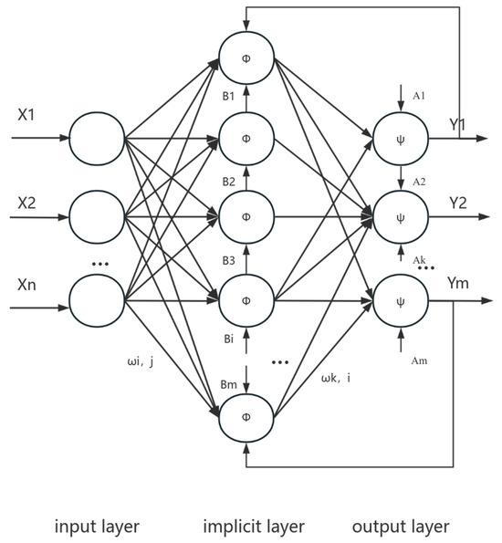
Figure 1.
Neural network topology.
In Figure 1, xj represents the input to the j-th node in the input layer, ωi,j denotes the weights between the i-th node of the hidden layer and the j-th node of the input layer, Bi is the threshold of the i-th node in the hidden layer, Φ represents the activation function of the hidden layer, ωk,i represents the weight between the k-th node in the output layer and the i-th node in the hidden layer, Ak is the threshold of the k-th node in the output layer, ψ is the activation function of the output layer, and Yk is the output of the k-th node in the output layer.
The computational steps of the BP neural network algorithm are as follows:
- (1)
- Forward propagation process
The input of the i-th node of the hidden layer is as follows:
The output of the i-th node in the hidden layer is as follows:
The input of the k-th node of the output layer and the output of the k-th node of the output layer are as follows:
- (2)
- Back propagation of error
The reverse transmission of this error starts from the output layer, calculates the error of each layer one by one, and then adjusts the weight and threshold of each layer by the error gradient method.
The error criterion function for sample p is
where represents the true value of the k-th sample. For P training samples, the overall error evaluation function of the system is as follows:
The learning rate is set, and the weights and thresholds are modified according to the gradient descent method.
where ′ means the derivative function.
Finally, the error can meet the accuracy requirements.
2.2. Principles of Genetic Algorithms
The genetic algorithm (GA) is a computational model established by Professor Holland [24] at the University of Michigan based on the principles of natural selection and genetic mechanisms described in Darwin’s theory of evolution [25]. It serves as an effective approach to simulate natural evolutionary processes for seeking optimization solutions. This algorithm operates by mimicking natural evolution and exploring multiple paths simultaneously without relying on prior system knowledge, which helps avoid getting trapped in local optima. Additionally, GA exhibits the following characteristics:
- (1)
- It starts from the solution set of a class of problems, covers a wide range, and facilitates global optimization.
- (2)
- Multiple schemes can be evaluated, and the algorithm itself is easy to parallel.
- (3)
- Only the adaptive function is used to evaluate the individual, and the application range is wide.
- (4)
- The probability transfer rule (probabilistic transfer rules are a way of describing the probability of state transfer for stochastic processes) is used to guide the search direction.
- (5)
- It has the ability to self-organize, self-adapt, and self-learn.
The genetic algorithm (GA) is a heuristic algorithm used for solving optimization problems. Its main objective is to manipulate the population based on their fitness evaluations (adaptation assessments) to achieve survival of the fittest. In essence, the computational process of a genetic algorithm involves generating an initial population P(t); evaluating this population; checking if termination criteria are met; and if not, generating a new generation of individuals through genetic operations (including selection, crossover, and mutation). This cycle continues iteratively until the termination criteria are satisfied [26]. Thus, in the operation of a genetic algorithm, obtaining the next generation population that meets the requirements through genetic operations is a crucial step in the algorithm.
The selection of individuals in evolutionary algorithms requires the evaluation of their fitness within the population. Existing selection methods include roulette wheel selection, fitness proportionate selection, and tournament selection, among others. Among these, the most common method is roulette wheel selection, whose calculation formula is illustrated as Equation (11):
Here, n represents the population size, fi denotes the fitness of individual i, and pi indicates the probability of being selected. As inferred from the above formula, when an individual has a higher fitness, its likelihood of being selected is also greater.
The concept of crossover involves exchanging and recombining certain structures between two parent individuals to generate a new offspring. Utilizing crossover operations enhances the optimization capability of the algorithm. Existing crossover operations can be categorized into real-value crossover and binary crossover based on the encoding format. Currently, the most common form of crossover is single-point crossover, which is a type of binary crossover. Its operation involves randomly selecting a crossover point on a single crossover sequence, then exchanging the segments before and after the crossover point to obtain a new individual.
In contrast to crossover operations, the distinction lies in mutation operators, which alter the value of a gene within the population. In practical applications, the most common mutation methods are real-value mutation and binary mutation. The specific operation process involves first determining whether mutation occurs based on a pre-set mutation probability, then selecting a mutation position randomly for individuals that undergo mutation.
2.3. Establishment of GA-BP Neural Network Model
In the training process of a back propagation (BP) neural network, the weights and thresholds are initially set randomly, which introduces a considerable degree of subjectivity. Inappropriate selection of these parameters can greatly affect the convergence and stability of the network. Additionally, employing a BP neural network for nonlinear optimization poses challenges such as low learning efficiency, slow convergence speed, and susceptibility to local minima [27].
Genetic algorithms possess strong overall search capabilities and optimization methods, and they do not rely on gradient information or other prior knowledge during computation. They demonstrate robustness across various problem types. Therefore, it is proposed to utilize genetic algorithms to optimize the weights and thresholds of BP neural networks, thereby enhancing the learning and generalization capabilities of BP neural networks. The schematic diagram illustrating the model construction process is depicted in Figure 2.
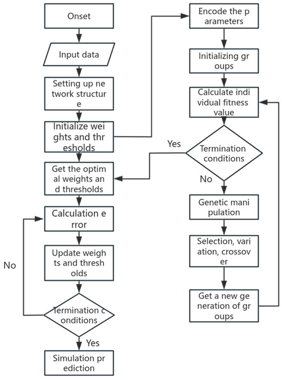
Figure 2.
Flowchart of GA-BP neural network algorithm.
The construction principle of this model is that first, the preprocessed data are input into the model set into the topological structure, the weights and thresholds obtained by iterative optimization of the genetic algorithm are assigned to the BP neural network, and then the final simulation results are obtained through the training and prediction of the neural network.
3. Case Analysis
3.1. Data Selecting
In order to verify the feasibility of the method proposed in this paper, experimental data from the literature on defect-containing pipelines were used for the study [28]. This dataset was derived from the full-scale blasting experiment. These data included the pipe diameter, wall thickness, tensile strength, yield strength, defect length, depth, width, and failure pressure. In the study presented in this paper, seven factors affecting pipeline failure, such as the pipe diameter, were taken as the input variables of the model, and the failure pressure was taken as the output variable of the model. The simulation prediction was carried out by using the BP neural network and the GA-BP neural network, and the prediction effect of the two methods was compared. The intercepted data are shown in the table below. From ref. [25], it can be seen that the failure pressure of the pipeline is related to the material of the pipeline and the characteristics of the defect area. Among them, the outer diameter of the pipe is the actual external size of the pipe; the wall thickness is the thickness of the pipe or pipe wall; and the length, width, and depth of the defect are the length, width, and depth of the defect area of the pipeline, respectively. The yield strength is the limit of the yield phenomenon of the material, that is, when the yield phenomenon of the pipeline occurs, it is the stress to resist the micro-deformation. Tensile strength is the maximum mechanical tensile stress that a material can be loaded. The failure pressure is the pressure at which the pipe fails. The flow of technology application is shown in Figure 3.
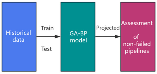
Figure 3.
Methodological applications.
Selected datasets are shown in Table 2.
Table 2.
Partial dataset.
3.2. Model Construction
3.2.1. Construction of BP Neural Network Model
The process of establishing a BP neural network mainly involves two parts: selecting the structure of the neural network and setting parameters. The neural network consists of three layers: the input layer, the hidden layer, and the output layer. Through analysis of the training samples, it was found that the input layer consisted of seven neurons, and the output layer consisted of one neuron. Based on the mapping theory of multi-layer neural networks, any continuous function can correspond to a three-layer neural network, that is, a three-layer neural network can solve most of the problems well [19]. Typically, an empirical formula is used to determine the number of nodes in the hidden layer [20]:
Or the number of hidden layer nodes is determined by the least square method:
In the equation, M represents the number of hidden layer nodes, n0 denotes the number of neurons in the output layer, n1 signifies the number of neurons in the input layer, and a is a constant ranging from 1 to 10.
Based on Equations (12) and (13), it can be inferred that in this study, the number of nodes in the neural network hidden layer ranged from 5 to 12.
Therefore, a three-layer neural network model was constructed in this study, with seven nodes in the input layer and one node in the output layer. Through repeated simulations and predictions, it was found that when the number of hidden layer nodes was set to 10, the model achieved the minimum mean square error. Consequently, the number of hidden layer nodes was set to 10. The training results of the model are presented in Table 2. The training iterations were set to 1000, with a learning rate of 0.01, and the training objective was to achieve a minimum error of 10−6. The errors for different numbers of hidden layers are shown in Table 3.
Table 3.
The training error when the hidden layer nodes are 5~12.
3.2.2. Parameter Selection of GA Algorithm
In this study, based on empirical methods, the initialization parameters of the genetic algorithm (GA) were set as follows: the initial population size was 30, the maximum number of evolutionary generations was 60, the crossover probability was set to 0.8, and the mutation probability was set to 0.2. The selection of individuals within the population was accomplished using the roulette wheel selection method. The next generation of the population was generated through two-point crossover and Gaussian mutation. Gaussian variation is a new mutation operation, which can replace the original gene with a random number satisfying the mean value of μ and the variance of σ2, thus improving the local optimization ability of the genetic algorithm. The specific formula is as follows [24]:
with the standard Gaussian probability density with and set to 0 and 1, respectively.
4. Results
The 60 sets of data were divided into two groups randomly, with 20 sets of data used as the training sample set and the remaining 40 sets of data used as the test set. The input and output data were normalized:
where x is the sample value after data normalization, X is the sample data, and Xmax and Xmin are the maximum and minimum values in the data. The BP neural network was constructed according to the parameter settings, the weights and thresholds were initialized, and each weight and threshold of the BP neural network was encoded as an individual in the genetic algorithm. The fitness function was used to find out the fitness of the individuals of the population, and they were compared. Then the next generation of individuals was updated by genetic operations (selection, crossover, and mutation operations). The iterations were stopped until the maximum number of iterations was satisfied or the accuracy requirement could be met; thus, the weights and thresholds of each layer of the BP neural network were obtained. The optimal weights and thresholds were then used to update the neural network, and finally, the simulation prediction was performed. Thus, the model algorithm evolution process diagram and GA-BP simulation prediction regression diagram are shown in Figure 4 and Figure 5.
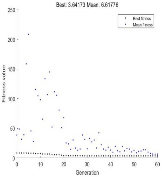
Figure 4.
Evolutionary process of the algorithm.
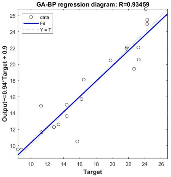
Figure 5.
Regression plot of GA-BP model prediction.
The maximum number of iterations for the model was set to 60, where the training error was taken as the mse fitness function. From the above figure, it can be observed that convergence was achieved after 40 iterations. At this point, the minimum fitness value was 3.61, and the average fitness value was 6.61. Additionally, from the GA-BP regression plot, it is evident that the model’s regression fitting rate was 0.93, demonstrating the feasibility of using the GA-BP neural network for pipeline failure prediction analysis.
5. Model Performance Analysis
As demonstrated in the previous section, using the GA-BP neural network for pipeline failure prediction is indeed feasible. However, relying solely on one model for prediction may not fully showcase the advantages of using the GA algorithm to optimize the BP neural network in pipeline failure prediction analysis. Therefore, this study employed the same structure of BP neural network to simulate and predict the same set of data and then compared the prediction results of the two models. This enabled the derivation of BP neural network regression plots, relative error curve plots for both models, and the relationship between the predicted values and the actual values. See Figure 6, Figure 7 and Figure 8 for details.
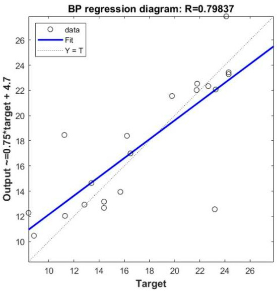
Figure 6.
Regression plot of BP model prediction.
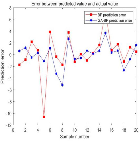
Figure 7.
Prediction errors of GA-BP vs. BP.
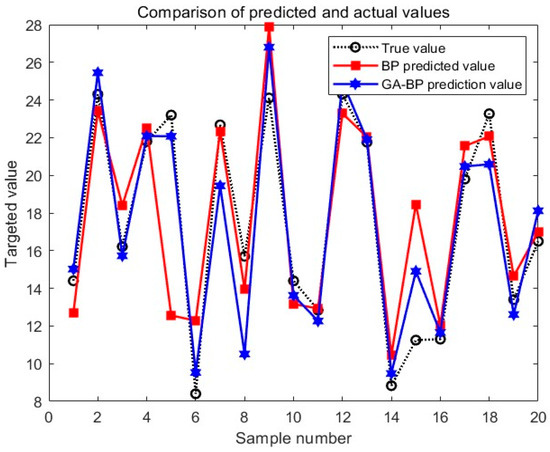
Figure 8.
Predicted values vs. actual values.
From the above graph, it can be observed that the regression coefficient obtained from simulating and predicting with the same structure of BP neural network was 0.798, indicating weaker regression fitting compared with the GA-BP neural network. By comparing the errors of the two models, it can be noted that the prediction error of the BP neural network fluctuated significantly, with the largest variation occurring when the sample number was 5. In contrast, the error variation of the GA-BP neural network was relatively low, and its maximum value was smaller than the maximum prediction error of the BP neural network. Through the comparison of the actual values, BP predicted values, and GA-BP predicted values, it became more intuitive that compared with the BP neural network model, the GA-BP model predicted failure pressure more accurately, with a smaller difference between the predicted and actual values and a better fitting effect. This demonstrated that the GA algorithm effectively reduced the error of the BP neural network, proving the superiority of using the GA algorithm to optimize the weights and thresholds of the BP neural network.
Additionally, this study employed the mean square error (MSE), root mean square error (RMSE), mean absolute percentage error (MAPE), and mean absolute error (MAE) to quantitatively evaluate the two models, with the formulas as follows:
Among them, yi is the true value of the failure pressure, is the predicted value of the failure pressure, and n represents the number of datasets. The four index values and differences of the GA-BP neural network model and BP neural network model are shown in the Table 4.
Table 4.
Comparison of errors between GA-BP and BP.
Based on the table above, it can be observed that all four error metrics of the GA-BP model were smaller than those of the BP model. Furthermore, among the two prediction models adopted in this study, the prediction accuracy of the GA-BP model was 91.15%, while that of the BP model was 86.87%. This indicated that the GA-BP model exhibited better fitting performance and higher prediction accuracy.
6. Conclusions
This paper presents a method for predicting pipeline failures. Due to the confidentiality of water supply pipeline data, which are not easily accessible, previous literature data were used to verify the feasibility of the proposed method. The genetic algorithm (GA) was applied to optimize the weights and thresholds of the BP neural network, resulting in a new BP neural network model. Simulated predictions were conducted using the same structured BP model on the same dataset, yielding the following conclusions:
- When setting parameters for the BP neural network, since the initial weights and thresholds of the BP neural network are randomly set, resulting in certain prediction errors, introducing the GA algorithm to optimize the weights and thresholds of the BP neural network can effectively reduce errors and improve the prediction accuracy of the model.
- This paper uses seven factors including the pipe diameter, wall thickness, tensile strength, yield strength, defect length, depth, and width as the failure factors of the pipeline. The prediction accuracy of the model is 91.15%. Therefore, the GA-BP neural network optimization algorithm proposed in this paper can be used for pipeline failure prediction research.
- Since training the network requires a large amount of data support, the accuracy of the data has a significant impact on the prediction accuracy of the model. The method proposed in this paper is only a preliminary study based on the available data. To improve the prediction accuracy of the model, further research is still needed.
Author Contributions
Conceptualization, Q.L.; methodology, Z.L.; software, Z.L.; formal analysis, Z.L.; writing—original draft preparation, Z.L.; writing—review and editing, Q.L.; visualization, Q.L.; All authors have read and agreed to the published version of the manuscript.
Funding
The National Key Research and Development Plan ‘Intelligent Sensing Technology and Equipment for Service Status of Urban Water Supply and Drainage Pipe Network’ (2022YFC3801000).
Data Availability Statement
All the data used in this study can be found in the article.
Conflicts of Interest
The authors declare no conflict of interest.
References
- Wang, T. Research on Pipe Burst Risk Prediction Model of Water Supply Pipe Network Based on BP Neural Network. Master’s Thesis, Chongqing University, Chongqing, China, 2019. [Google Scholar]
- Zhang, H. Research and Application of Pipeline Risk Evaluation in Urban Water Supply Networks. Master’s Thesis, Changán University, Xi’an, China, 2020. [Google Scholar]
- Jing, Y. Optimal Scheduling of Urban Water Supply Network Systems Considering Failure Risk Assessment Factors. Master’s Thesis, Harbin Institute of Technology, Harbin, China, 2021. [Google Scholar]
- Wang, C. Research on Risk Evaluation of Water Supply Pipelines Based on Bayesian Theory. Ph.D. Thesis, Tianjin University, Tianjin, China, 2010. [Google Scholar]
- Qing, X.; Zhao, X.; Zhang, H.; Tian, Y. Pipe burst prediction model for water supply network. China Water Supply Drain. 2012, 28, 68–71. [Google Scholar]
- Yang, Y.; He, K.; Ji, J.; Tan, Y.; Xu, S.; Zhang, K. Gray cast pipe failure prediction model in water distribution system based on Zero-inflated Poisson model. J. Cent. South Univ. Sci. Technol. 2022, 53, 560–568. [Google Scholar]
- Demissie, G.; Tesfamariam, S.; Sadiq, R. Prediction of Pipe Failure by Considering Time-Dependent Factors: Dynamic Bayesian Belief Network Model. ASCE-ASME J. Risk Uncertain. Eng. Syst. Part A-Civ. Eng. 2017, 3, 04017017. [Google Scholar] [CrossRef]
- Thi Minh Lanh, P.; Hai Ha, P.; Nguyen Anh Thu, D.; Dinh Hong, L. Proposed probabilistic models of pipe failure in water distribution system. MATEC Web Conf. 2018, 193, 02002. [Google Scholar] [CrossRef][Green Version]
- Burn, S.; Davis, P.; Gould, S. Risk Analysis for Pipeline Assets-The Use of Models for Failure Prediction in Plastics Pipelines. In Proceedings of the 4th International Symposium on Service Life Prediction, Key Largo, FL, USA, 3–8 December 2009; pp. 183–204. [Google Scholar]
- Hajali, M.; Shdid, C.A. Using numerical modeling for asset management of buried prestressed concrete cylinder pipes. Struct. Concr. 2020, 22, 1487–1499. [Google Scholar] [CrossRef]
- Xu, W.-Z.; Li, C.B.; Choung, J.; Lee, J.-M. Corroded pipeline failure analysis using artificial neural network scheme. Adv. Eng. Softw. 2017, 112, 255–266. [Google Scholar] [CrossRef]
- Peng, S.; Cheng, R.; Wu, Q.; Cheng, J.; Meng, T. Research on pipe burst identification in water supply network based on extreme learning machine algorithm. China Water Supply Drain. 2022, 38, 56–62. [Google Scholar] [CrossRef]
- Qi, F.; Kam, B.; Cheng, T.; Ma, W.; Yao, T.; Wang, K. Failure prediction and sensitivity analysis of pipe girth welds based on neural network. J. Southwest Univ. (Nat. Sci. Ed.) 2024, 46, 159–167. [Google Scholar] [CrossRef]
- Asnaashari, A.; McBean, E.A.; Gharabaghi, B.; Tutt, D. Forecasting watermain failure using artificial neural network modelling. Can. Water Resour. J. 2013, 38, 24–33. [Google Scholar] [CrossRef]
- Hoseingholi, P.; Moeini, R. Pipe failure prediction of wastewater network using genetic programming: Proposing three approaches. Ain Shams Eng. J. 2023, 14, 101958. [Google Scholar] [CrossRef]
- Liu, W.; Liu, Z.; Liu, Z.; Xiong, S.; Zhang, S. Random Forest and Whale Optimization Algorithm to Predict the Invalidation Risk of Backfilling Pipeline. Mathematics 2023, 11, 1636. [Google Scholar] [CrossRef]
- Li, X.; Jing, H.; Liu, X.; Chen, G.; Han, L. The prediction analysis of failure pressure of pipelines with axial double corrosion defects in cold regions based on the BP neural network. Int. J. Press. Vessel. Pip. 2023, 202, 104907. [Google Scholar] [CrossRef]
- Zali, R.B.; Latifi, M.; Javadi, A.A.; Farmani, R. Semisupervised Clustering Approach for Pipe Failure Prediction with Imbalanced Data Set. J. Water Resour. Plan. Manag. 2024, 150, 04023078. [Google Scholar] [CrossRef]
- Zhang, T.; Shuai, J.; Shuai, Y.; Hua, L.; Xu, K.; Xie, D.; Mei, Y. Efficient prediction method of triple failure pressure for corroded pipelines under complex loads based on a backpropagation neural network. Reliab. Eng. Syst. Saf. 2023, 231, 108990. [Google Scholar] [CrossRef]
- Geem, Z.W.; Tseng, C.L.; Kim, J.; Bae, C. Trenchless Water Pipe Condition Assessment Using Artificial Neural Network. In Pipelines 2007: Advances and Experiences with Trenchless Pipeline Projects—Proceedings of the ASCE International Conference on Pipeline Engineering and Construction; American Society of Civil Engineers (ASCE): Charleston, SC, USA, 2012. [Google Scholar]
- Cho, Y.T.; Lee, G.H.; Hong, J.-H.; Woo, G.Z. Prediction of Photovoltaic Generation Using Machine Learning Models with Various Weight Optimization Techniques. J. Korean Inst. Intell. Syst. 2022, 32, 1–6. [Google Scholar]
- Shirzad, A.; Safari, M.J.S. Pipe failure rate prediction in water distribution networks using multivariate adaptive regression splines and random forest techniques. Urban Water J. 2019, 16, 653–661. [Google Scholar] [CrossRef]
- Verheugd, J.; da Costa, P.R.D.; Afshar, R.R.; Zhang, Y.Q.; Boersma, S. Predicting Water Pipe Failures with a Recurrent Neural Hawkes Process Model. In Proceedings of the IEEE International Conference on Systems, Man, and Cybernetics (SMC), Electr Network, Toronto, ON, Canada, 11–14 October 2020; pp. 2628–2633. [Google Scholar]
- Wen, Z.; Sun, H.K. MATLAB Intelligent Algorithms; Tsinghua University Press: Beijing, China, 2017. [Google Scholar]
- Yue, S.; He, S.; Wang, G.; Liu, W.; Chen, C. Research on Optimal Deployment Problem of Weapon System Based on Improved Genetic Bee Colony Algorithm. J. Weapons Equip. Eng. 2022, 43, 80–86. [Google Scholar]
- Zhao, Y.; Ru, T. Comparative Analysis of Implementation and Performance of Genetic Algorithm for Small Habitat with Shared Adaptation Value. J. Tonghua Norm. Coll. 2014, 35, 48–50. [Google Scholar] [CrossRef]
- Zhang, X.S.; Zhang, Y. Prediction of failure pressure of corroded pipeline based on Lasso-PSO-BP neural network. Mater. Prot. 2020, 53, 46–52. [Google Scholar] [CrossRef]
- Shen, X. Prediction of Girth Weld Defect Failure of Long Distance Pipeline. Master’s Thesis, Xi’an Shiyou University, Xi’an, China, 2022. [Google Scholar]


Disclaimer/Publisher’s Note: The statements, opinions and data contained in all publications are solely those of the individual author(s) and contributor(s) and not of MDPI and/or the editor(s). MDPI and/or the editor(s) disclaim responsibility for any injury to people or property resulting from any ideas, methods, instructions or products referred to in the content. |
© 2024 by the authors. Licensee MDPI, Basel, Switzerland. This article is an open access article distributed under the terms and conditions of the Creative Commons Attribution (CC BY) license (https://creativecommons.org/licenses/by/4.0/).