Abstract
The adoption of green roofs is an effective practice for mitigating environmental issues in urban areas caused by extreme weather conditions. However, certain design aspects of green roofs, such as the characterization of the physical properties of their substrates, need a better understanding. This study proposes a simple method for estimating two hydraulic properties of green roof substrates based on the evolution of moisture during drying periods, or drydowns, where evaporative processes dominate: the weighted-mean diffusivity and the saturated hydraulic conductivity. Soil moisture was monitored using 12 in situ sensors from 2015 to 2020 in a study involving six different green roof plots composed of various mixtures of demolition-recycled aggregates and organic substrates. A universal parameterization for determining water diffusivity in soils was applied to estimate the weighted-mean hydraulic diffusivity. As a by-product, the saturated hydraulic conductivity was estimated from the evaluated diffusivity and the measured water retention data. The median values obtained for and range from 14.5 to 29.9 cm2d−1 and from 22 to 361 cmd−1, respectively. These values fall within the ranges reported by other research groups using direct measurement methods and supports the validity of Brutsaert’s model for green roof substrates. Furthermore, an increase in and a decrease in were observed as the percentage of recycled aggregates in the substrates increased, which could be considered for design purposes.
1. Introduction
The progressive increase in temperature, particularly in urban environments, the growing concern to improve living conditions in highly populated areas, and the results of previous experiments worldwide have led to the proliferation of urban surfaces covered with vegetation. This has prompted the study of their properties, as seen in studies such as those of Jacobs et al. [1] and Alim et al. [2] on green roofs.
A green roof consists essentially of a surface layer usually occupied by plants, a growing medium that is in most cases some organic substrate, a filter typically consisting of geotextiles, a drainage store, and a root barrier overlying a waterproofing membrane, e.g., [3]. As Mihalakakou et al. [4] indicated, green roofs serve multiple purposes: they save energy, maintain the quality of air, conserve water, mitigate streets flooding, enhance biodiversity, and attenuate urban noise, among other effects. They also contribute to the mitigation of energy transfer rates between them and the atmosphere [5], the dissipation of part of the incoming net radiation to maintain air temperature in a reduced interval [6], the filtration of part of rain-leached atmospheric pollutants, the reduction of noise [7], and the improvement in water quality in urban runoff [8,9,10].
In the green roof modelling literature, hydrological behavior is usually defined by retention and detention processes. Detention is understood as the delay and attenuation of the runoff hydrograph, and retention is understood as the amount of rainfall intercepted by the green roof system [11]. Numerous studies have highlighted the reduction in runoff volumes, the decrease in peak runoff rates, and the delay in hydrograph response, e.g., [12,13,14]. Simple models such as the Thornthwaite–Mather model (TMM) and the description by McColl et al. [15] can be used. Several models assimilate the green roof to a bucket, a single store with either a linear or non-linear relationship between storage volumes and discharge rates. Lucatelli et al. [16] and Vesuviano et al. [17] chose the non-linear model, decomposing the store in two parts, one for the root system and the other for the percolated water. Some authors, such as Carson et al. [18], found that the Soil Curve Number method successfully estimated the conversion of gross rainfall to runoff for several green roofs in New York City. Therefore, most of the precipitation of rainfall events below a certain threshold could be retained; Castro et al. [19], for instance, suggested up to 22 mm of retention for a certain green roof set-up, and Kemp et al. [20] suggested up to 18% of the received rain depth. She and Pang [21] used the Green and Ampt [22] model to follow water’s infiltration into a growing media. Cascone et al. [23] and Ebrahimian [24] summarized the evapotranspiration processes in green roofs. Starry et al. [25] applied the Penman–Monteith equation according to FAO standards [26] with seasonal crop coefficients for different green roof plants. Stovin et al. [27] and Berretta et al. [28] estimated the actual evapotranspiration rate as proportional to the ET0, corrected by the ratio of the measured water content of the growing media and its maximum value, called by them ‘field capacity’, a kind of effective saturation degree [29] that is similar to the Thornthwaite and Mather (TMM) proposal, for the formulation of their water balance model [30].
Previous approaches have typically relied on empirical soil moisture extraction functions to factor the substrate moisture content to allow actual ET losses to be estimated from a reference ET. But such functions do not account for substrate-specific moisture release characteristics. The use of more complex models such as the Richards equation for soil water movement could also be appropriate, e.g., Gardner’s [31] desorption. Some works have used complete soil water and heat flow models like HYDRUS-1D [32] or HYDRUS-2D [33] to interpret the behavior of green roofs. Carbone et al. [34] described a small-scale analogic model and Sandoval et al. [33] even adapted a complete soil moisture model to explore the possibilities of green roofs in Chile. But these types of models might not always be practical in extensive green roofs due to their required number of parameters. The reduced depth of the growing media and the large horizontal extent of the plots could suggest the adoption of simpler models that require a smaller number of parameters to describe the hydraulic properties of green roof substrates.
The optimal substrate for green roofs varies with climate. In Mediterranean areas, characterized by prolonged and rainless summers, the substrate must be able to avoid flooding during heavy rainfalls but also retain moisture during the dry season to allow the survival of vegetation. Thus, the selection of the substrate is a key factor for the success of the system. There are many papers dedicated to substrates, e.g., [35]. Some focus in detail on the hydrophysical characterization of green roof substrates, with extended discussions on the soil water retention curve (SWRC) and unsaturated hydraulic conductivity function (HCF), e.g., [36,37]. According to Fassman-Beck et al. [38], the most relevant factor for runoff mitigation is the horizontal flow path length through the drainage layer to vertical gutters, as well as the roughness of this layer, dominated by the substrate. Kader et al. [39] proposed a drought tolerance test consisting of a platform to test the ability of plants to resist extreme drought conditions. More formal methods were suggested by Coelho et al. [40] for the estimation of water vapor transmission, hygroscopic sorption, and water retention and drainage capacity; and by Sandoval et al. [33], who used the Hydrus model to estimate some optimal compositions of the substrate mixture, i.e., peat and inert, gravel, and material. Whilst these papers have mainly focused on the importance of these physical characteristics for controlling the runoff/percolation rate, observations of physical characteristics are equally relevant to soil moisture losses due to ET.
The use of recycled aggregates (RAs) as green roof substrates has been recently incorporated, e.g., [36,41], with a twofold purpose to obtain an optimal porous medium, increasing pore size, and to eliminate residues which could become a nuisance. López-Uceda et al. [42] rationalized the use of RAs in green roofs and analyzed the leaching risk of the substrate object of this study. It was confirmed that the use of recycled aggregates complies with non-polluting effluent regulations. But their effectiveness as a support for vegetation in terms of water properties was not analyzed.
From the analysis of the vertically integrated water budget for a soil, Laio et al. [43] stated that the temporal variation in the moisture content was equal to the rainfall minus the loss rate. The loss rate can be composed of percolation, runoff, and evapotranspiration, but a certain time after a precipitation event, it corresponds essentially to the evaporation, and, more properly, to stage II of the evaporation, where soil controls the process.
The description of the evaporation process, which usually predominates over drainage in Mediterranean regions, can be a key element of the characterization of the substrates, as recommended by McColl et al. [15], who coined the term “drydown” to represent a quasi-permanent characteristic of the land surface. The drydowns correspond roughly to the second stage of soil water evaporation (e.g., [44]) and depend on a time factor, a flux rate reference, and the limits of the moisture interval. The time factor is related to the memory of the soil of the surface soil moisture, a timescale required for the dissipation of a perturbation like a rain event, and, consequently, a characteristic of the substrate (e.g., [45]).
In a few cases, drying periods have been used to analyze the soil response, as in Berretta et al. [28] or [46], who measured and estimated evapotranspiration in their experiments to assess the suitability of green roofs in different areas of the United Kingdom. Brutsaert [47,48] presented a universal parameterization of the daily evaporation from a soil, considered as an isothermal linear diffusion process in a bounded medium. For such a purpose, he adopted the weighted-mean diffusivity proposed by Crank [49] and first used by Gardner [31] for the analysis of soil water evaporation to simplify the complexity of the problem.
The purpose of this paper is to estimate some of the hydrophysical properties of green roof substrates based on the evolution of moisture during the drying periods, or drydowns, where evaporative processes dominate. To achieve this, the weighted-mean water diffusivity of green roof substrates will be estimated using the method developed and applied to natural soils by Brutsaert [47] based on the moisture data acquired by electromagnetic sensors in a green roof experiment in Córdoba, Southern Spain, maintained during a 6-year period. To verify the consistency of the results, the saturated hydraulic conductivity of the substrates will be determined by comparing the weighted-mean diffusivity estimates obtained using the Brutsaert [47] method with the estimates computed from the soil water retention curve proposed by van Genuchten [50].
2. Materials and Methods
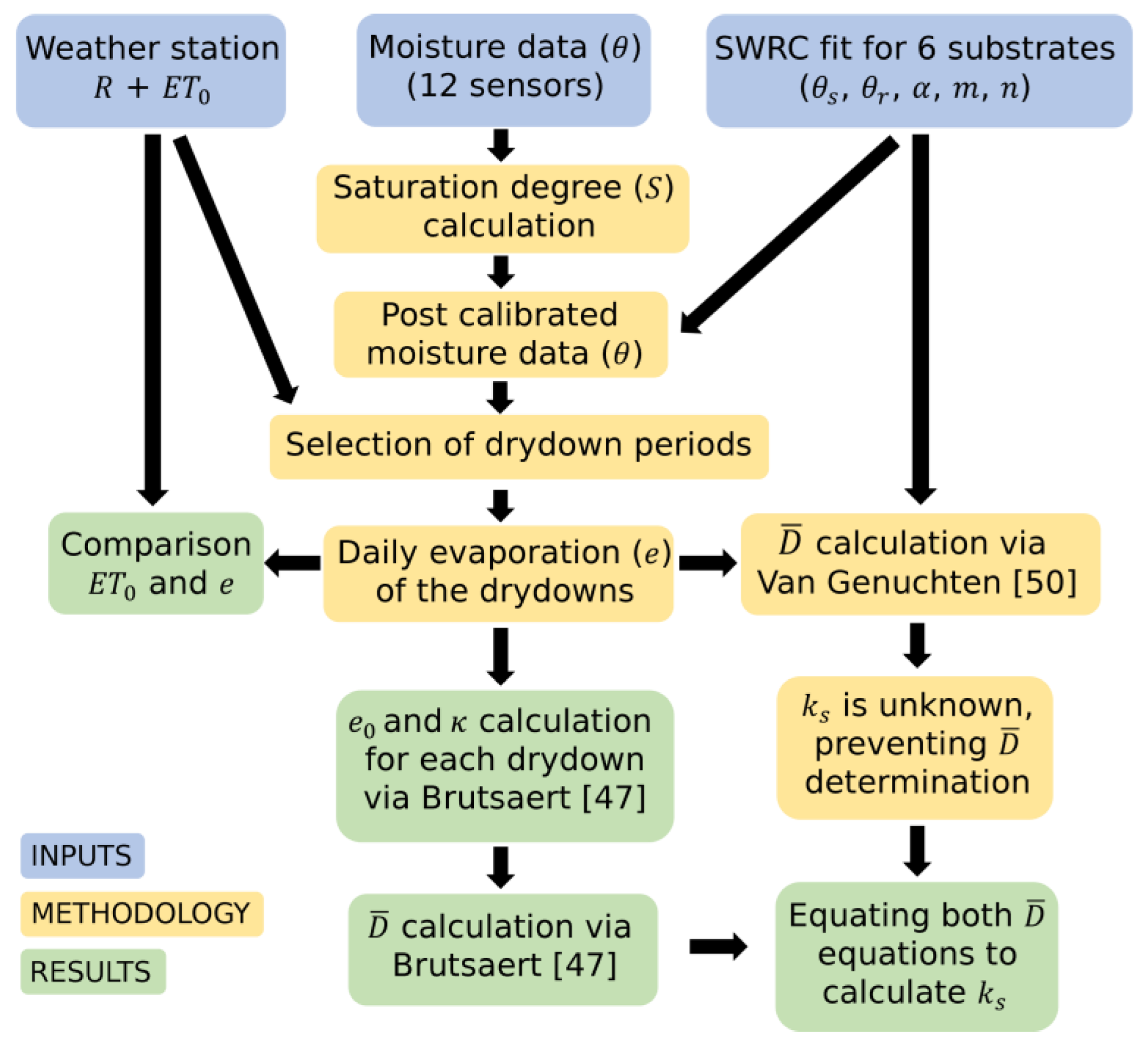
A green roof experiment was set up on one building of the campus of the University of Cordoba (Section 2.1); it was equipped with moisture sensors (Section 2.2), and the soil water retention curve of the substrates was measured in the laboratory (Section 2.3). Inverse normalization was used to compensate for the absence of a site-specific moisture calibration (Section 2.4). The characterization of the hydrophysical properties of the green roof substrates was carried out during evaporation periods, also referred to as drying periods or drydowns (Section 2.5); specifically, weighted-mean diffusivity (Section 2.6) and saturated hydraulic conductivity (Section 2.7) were evaluated. In Section 2.6, a soil water evaporation model was applied to identify the initial evaporation intensity and reference time present in the Brutsaert [47] model to finally calculate the weighted-mean diffusivity, which can be a good indicator of the hydrophysical properties of green roof substrates. The weighted-mean diffusivity can be characterized with other means. In Section 2.7, for instance, the method reported by Crank [49] and van Genuchten [50] was used based on the water retention curve. This alternative method offers the possibility to estimate the value of the saturated hydraulic conductivity. The conceptual road map followed in the mentioned analysis is presented in Figure 1.

Figure 1.
Conceptual figure of the road map followed for calculations. Symbols used in this figure are rainfall (R), reference evapotranspiration (ETo), soil moisture (θ), soil saturation degree (S), evaporation (e), the reference evaporation rate (e0) and time (κ) from the Brutsaert [47] method, as well as, weighted-mean diffusivity (), saturated hydraulic conductivity (), and the soil water retention curve (SWRC) with its correspondent values of residual water content (θr), saturated water content (θs), a scaling parameter (α), and shape parameters (m, n).
2.1. Green Roof Set-Up
At the beginning of spring 2015, six extensive green roofs plots 4.4 × 3.2 m2 in size and containing different substrates were installed on a building on the University of Cordoba campus (37.92° N, 4.72° W, 136 masl), as seen in Figure 2. The depth of the growing media was initially 0.10 m. The climate in Cordoba is Mediterranean, Csa in the Köppen–Geiger scheme [51]. Agrometeorological information, namely, air temperatures, reference evapotranspiration rates (ETos), and rainfall rates, were collected from an automatic station called “UCO-B.G. Olivo” (37.93° N 4.72° W), located within 200 m from the study site [52]. In this location, the mean annual temperature is 18.5 °C, with a long, hot summer and fluctuations between the average of the annual minimum daily values in winter, −2.1 °C, and the average of the annual maximum daily values in summer, 42.6 °C. The average annual precipitation is 530 mm, with 80% of the rain concentrated in the fall and winter seasons, from October to March, and the average annual potential evapotranspiration is 1313 mm.
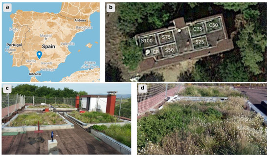
Figure 2.
Location and appearance of the six green roof plots and the reference plot installed on a building of the University of Cordoba. (a) Location on the map, and (b) situation on the roof of the building [53] and plot identification. (c,d) Appearance of the plots.
Six substrates composed of mixtures in different proportions of recycled aggregates and organic substrates were tested. The properties of the growing media are summarized in Table 1. The recycled aggregates (RAs) consist of recycled sand obtained in a construction and demolition waste treatment plant, containing ceramic, concrete, gypsum, and other residues, with a maximum particle size of 8 mm and a sandy texture. The commercial substrate S, recommended for roof gardens, consists of organic material (mull, coconut) and volcanic tuff, and has a sandy texture. Substrate C is composted mulch used for organic cropping, and comprises 100% composted organic matter. The bulk density was measured in 2019 by standard methods [54] (§ 2.1).

Table 1.
Green roof growing media composition, bulk density, and thickness.
A selection of plant species with shallow rooting systems and moderate development of aerial parts was adopted (e.g., [55]). A mixture of Acinos alpinus, Trifolium repens, Phagnalon saxatile, Lobularia maritima, Sedum sediforme, Cerastium tomentosum, Lotus corniculatus, Sanguisorba minor, Paronychia argentea, Brachypodium retusum, Bellis perennis, and Dianthus arenarius was sown. During the hot season, an automatic drip irrigation system supplies approximately 4 l m−2 of water to the plants daily. An outlet on the side of each plot and below the height of the drainage layer directs runoff water to a tank located on the ground floor of the building. The experimental plots have a 0.08 slope toward the outlet.
2.2. Monitoring in the Set-Up
Water content and temperature were monitored every 15 min with (i) two Campbell CS616 moisture sensors and (ii) ten Campbell 107 thermistors in each plot. The aim was to characterize through different studies the water and energy balances, and the efficiency of different substrate mixtures to reduce the impact of incoming radiation into the building underneath. The sensors’ arrangement in and the schematic cross-section of each plot are shown in Figure 3.
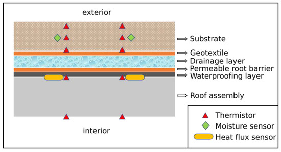
Figure 3.
Schematic vertical cross-section of each plot structure and sensor distribution.
The water content was averaged daily from the measures and recorded every 15 min. The data were treated separately in the two moisture sensors of each plot, resulting in 12 daily datasets.
Linear standard calibration from Campbell was applied to the data collected with the moisture sensors, preceded by a temperature calibration [56], obtaining the volumetric .
2.3. Water Retention Curves
The soil water retention curve of the substrates was measured in the laboratory using the standard methods [57] (§ 3.3.2). Experimental data were measured by Montes [58] during the year 2019 with a sand suction table, a kaolin suction table, and a WP4 psychrometer.
The van Genuchten [50] soil water retention equation, written in terms of a water saturation degree or normalized humidity, S (Equation (1)), was fitted to the moisture content, θ, and the matric or suction component of the soil water potential, ψ, using the curve_fit function from the SciPy library for Python [59] based on the Levenberg–Marquardt optimization algorithm [60]. The relevant parameters were the residual water content, θr, the saturated water content, θs, a scaling parameter, α, and a shape parameter, n. An additional shape parameter, m, adopts the value m = 1 − 1/n to simplify the hydraulic conductivity expression [50].
2.4. Moisture Site-Specific Calibration
On-site substrate-specific calibrations were not undertaken a priori. To address this issue, the obtained water content () was written in terms of the water saturation degree or normalized humidity, S, using the actual moisture content (), the residual moisture content (), understood as the minimum value, and the saturation moisture content (), understood as the maximum value in every sensor, defined by Equation (2).
With the saturation and residual moisture from the water retention curves in each substrate, substrate-specific calibration of the moisture sensor data was carried out through inverse normalization, obtaining the considered substrate’s calibrated θ value (Equation (3)).
2.5. Selection of Soil Moisture Drydowns
Evaporation periods, also referred to as drying periods or drydowns, were methodically extracted from the moisture database, spanning from the year 2015 to 2020. The daily evapotranspiration intensity, denoted as , was estimated as the difference between the mean daily values of measured soil moisture for each two consecutive days (Equation (4)).
where is the day, is the substrate depth, and are the mean moisture in the day and the day after, respectively.
The drydown periods were filtered for periods of continuous water loss of 4 days or more, with neither precipitation nor irrigation. The values of each period were compared with those of the reference evapotranspiration rates (ETos) from the nearby weather station.
2.6. Soil Water Evaporation Modeling Applied to Green Roofs
As Brutsaert [47] explained, water evaporation from a porous medium of finite depth underlain by a plane of zero flux can be characterized by the Richards, or Richardson and Richards, equation [61], neglecting the gradient of the gravitational component of the water potential in vertical flow (Equation (5)). This equation, with the depth z, volumetric moisture content θ, and time t, incorporates the matric potential component of water in the medium, ψm = −h, and the hydraulic conductivity, k. Additionally, the introduction of soil water diffusivity, D (Equation (6)), reduces the dependent variables of soil moisture, θ.
The term diffusivity D is defined as the product of the hydraulic conductivity, k, and the slope of the soil water retention curve, dψ/dθ. This equation is subject to initial and boundary conditions (Equation (7)) corresponding to the second stage of evaporation, controlled by the soil properties. The initial condition corresponds to a uniformly distributed water content in the substrate θini. Boundary conditions include a fixed moisture value in the surface of the substrate, , and a zero-flux plane depth, , and t is the time. Although the boundary condition at the zero-flux plane depth may appear somewhat limiting, Brutsaert [48] later demonstrated that the solution to Equation (5) produces similar results when a constant zero-flux plane depth is fixed.
To solve Equation (5), a linearization or conversion to a linear form can be employed, following the approach introduced by Crank [49]. This involves utilizing a weighted-mean value of the diffusion coefficient, referred to as the weighted-mean diffusivity, . Gardner and Mayhugh [62], and particularly Gardner [31], successfully applied the weighted-mean diffusivity in soil physics to obtain an analytical solution of the water movement.
To calculate the daily evolution of evaporation intensity instead of examining the evolution of moisture profiles in the substrate, Brutsaert [47] solved the Richards equation, Equation (5), with the Laplace transform [63], leading to Equation (8). The evaporative flux, e, can be expressed as the product of the weighted-mean diffusivity, , and the moisture gradient at the substrate surface, z = 0.
In Equation (8), represents the initial evaporation rate, and the reference time. And its solution for long periods can be reduced to Equation (9).
According to Equation (9), Brutsaert’s parameters e0 and κ can be determined by establishing a linear relationship between the logarithm of the evaporation rate e and the time (Equation (10)). During the second stage of the evaporation, e0 is obtained from the ordinate at the intercept, and κ is calculated as the inverse of the slope of the fitted linear relationship.
In this study, both parameters, e0 and κ, were evaluated with a simple linear regression fit during drydowns, using the daily evolution of substrate evaporation derived from the moisture measurements made by the sensors installed in the substrates.
A statistical analysis to evaluate the exponential fit of with time was carried out with the MSE, F-test, and its probability (e.g., [64] (§ 7.2.5)) to reduce errors related with the potential presence of other components of the loss function in certain drydown periods.
Additionally, Brutsaert [47] indicated that the two parameters and are related to the weighted-mean diffusivity , the zero-flux plane depth , and the two characteristic moisture contents and .
Therefore, squaring Equation (11) and multiplying it by Equation (12), the weighted-mean diffusivity can be written as a function of the parameters and (Equation (13)). Subsequently, the weighted-mean diffusivity can be inferred from the moisture sensor data for each drydown.
2.7. Assessment of the Weighted-Mean Diffusivity Based on the Water Retention Curve Parameters for the Estimation of the Saturated Hydraulic Conductivity
An alternative method to obtain the weighted-mean diffusivity is a direct evaluation from the soil water retention and the hydraulic conductivity equations. The diffusivity depends on the hydraulic conductivity and the slope of the soil water retention curve, as defined by Equation (14), e.g., [65] (§ 5.3).
Therefore, by coupling the van Genuchten soil water retention function with the Mualem hydraulic conductivity function, known as the van Genuchten–Mualem hydraulic conductivity function [50], the water diffusivity can be determined (Equation (15)).
In Equation (15), represents the saturated hydraulic conductivity, S is the water saturation degree (Equation (1)), and α and m are the van Genuchten soil water retention parameters. The only unknown parameter is precisely the saturated hydraulic conductivity, .
The weighted-mean diffusivity formulated by Crank [49] and coined by Brutsaert [47] can be estimated for each drydown by integrating it with the parameter and with the moisture content limits and .
The integral of Equation (16) does not have a known general analytical solution since the form of the diffusivity might be any function. Some works, e.g., [31,66], fitted an exponential function to the experimentally evaluated data. Brutsaert [47] applied a diffusivity function that had an exact solution for the water desorption process to give a proper estimate of the value of the coefficient, ≈ 1.77.
Introducing the moisture normalized values, , , (Equations (1) and (17)) in Equation (19) using the residual moisture, , and saturated moisture, , from the retention curve, the final formulation of the weighted-mean diffusivity for the interval to is derived, as presented in Equation (18).
Substituting the expression of the soil water diffusivity (Equation (15)) into the latter equation (Equation (18)) yields a final expression for the weighted-mean diffusivity (Equation (19)).
If we assume, as Brutsaert [47] did, a power relationship between the normalized moisture, S, and diffusivity, D, in Equation (15), the integration can be solved with the assistance of the incomplete beta function [67] (§ 6.6). However, if this hypothesis is not acceptable, a straightforward numerical integration, such as Gauss–Legendre, e.g., [68] (§ 4.5), can estimate the value of the method used in this case study.
Without previous knowledge of the saturated hydraulic conductivity, , it is possible to evaluate it by comparing Equation (19) with Equation (13), yielding Equation (20), where represents the obtained with the Brutsaert (2014a) method and represents the value obtained with the integration of Equation (19) from the van Genuchten [50] and Crank [49] method.
2.8. Comparison of the Weighted-Mean Diffusivities of the Different Substrates
Will the weighted-mean diffusivity discriminate between different substrates? To answer this question, the estimated values of the weighted-mean diffusivity must be compared. For such a purpose, given the different size of the sets of data for each substrate, some nonparametric tests were chosen, e.g., [64] (§ 5.3.1). The Kruskal and Wallis test is, as indicated by Conover [69] (§ 5.2), a good exploratory tool to check if the data of different statistical populations, in this case corresponding to the different substrates, proceed from the same ensemble. The resulting statistic is based on the ranks of observations of a mixture of all the sets of data, or substrates used. This statistic tests the null hypothesis that all the sets have the same mean. In the case that the probability associated with this statistic is smaller than 0.05, the null hypothesis will be rejected. If the equality of all means is rejected, the sets of the data obtained in each sensor should be compared pairwise with the test of Mann–Whitney [69] (§ 5.1).
3. Results and Discussion
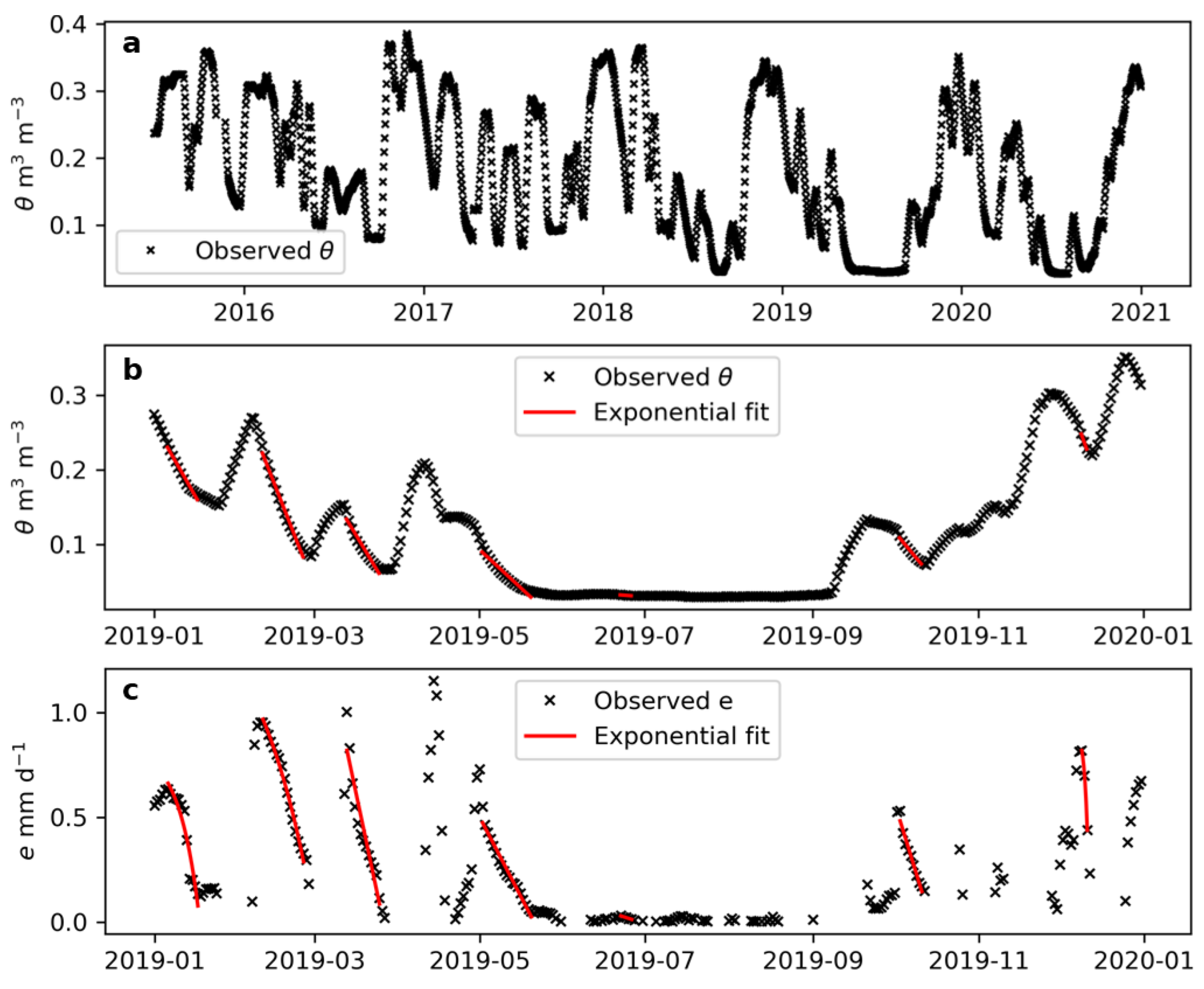
Daily moisture and evaporation from each sensor were analyzed, as shown in Figure 4, for one sensor in one single year. The evolution of moisture content is similar in all the plots. Moisture increases quickly in response to the rainfall pulses, partially due to the thinness of the substrate. The drying processes are slightly slower, indicating the control of the process by the substrate.
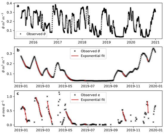
Figure 4.
(a) Evolution of moisture for the west moisture sensor of plot C75, (b) observed moisture for the same sensor in one year, 2019, and (c) obtained daily evaporation for the same year and sensor. In b and c, the red lines show the exponential fits of the 7 drydown periods identified.
A total of 447 drydown periods were obtained for all years and sensors. The average values (Table 2) show the expected variability during the different seasons; moisture content is lower in summer and higher in winter, which is opposite to air temperature and the average ETo, being higher in summer and lower in winter.
Table 2.
Summary of moisture drydowns extracted for the analysis from year 2015 to 2020, grouped by season.
3.1. Water Retention Curve Parameters
The values of the van Genuchten water retention curve parameters for each substrate are gathered in Table 3. The goodness of fit of the van Genuchten equation to the laboratory-measured data achieved a mean value of the Nash–Sutcliffe efficiency coefficient of 0.97.
Table 3.
Green roof growing media properties. is residual moisture, is saturation moisture, α, n, and m are van Genuchten soil water retention parameters, where .
To check the relationships between the different parameters, the matrix of correlations between them is computed in Table 4, showing coherent results.
Table 4.
Correlation matrix for the values of the parameters of the van Genuchten soil water retention equation: α, n, the residual moisture , and saturated moisture, .
3.2. Parameter Estimation of the Brutsaert [47] Soil Water Evaporation Model
The values for the reference evaporation rate (e0) and time (κ) were obtained for all drydowns. Their mean, median value, and standard deviation for each plot appear in Table 5.
Table 5.
Mean, median, and standard deviation of the reference evaporation rate (e0) and reference time (κ) from the Brutsaert equation [47] for each substrate.
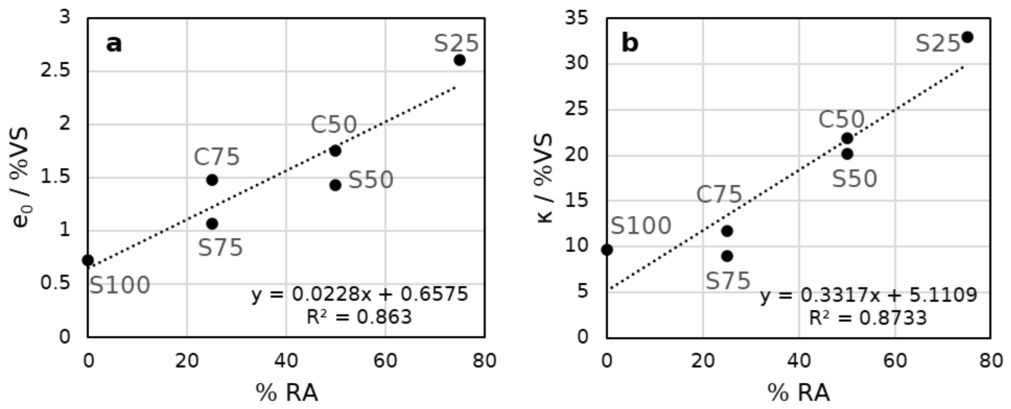
The results are of the same order of magnitude as the data found by Brutsaert [47] for field soils. If the parameter values are normalized by the fraction of the vegetative substrates (VS) S and C and plotted against either the percentage of vegetative substrates or aggregates (Figure 5), a notable relationship emerges where e0 and κ increase with the percentage of recycled aggregates. This approach emphasizes the main role of the vegetative substrate in the evaporation process.
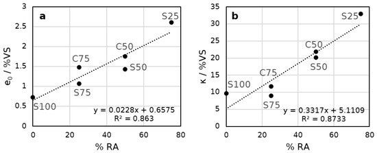
Figure 5.
(a) Reference evaporation (e0) normalized with the fraction of vegetative substrates and compared with the fraction of recycled aggregates. (b) Reference time (κ) normalized with the fraction of vegetative substrates and compared with the fraction of recycled aggregates.
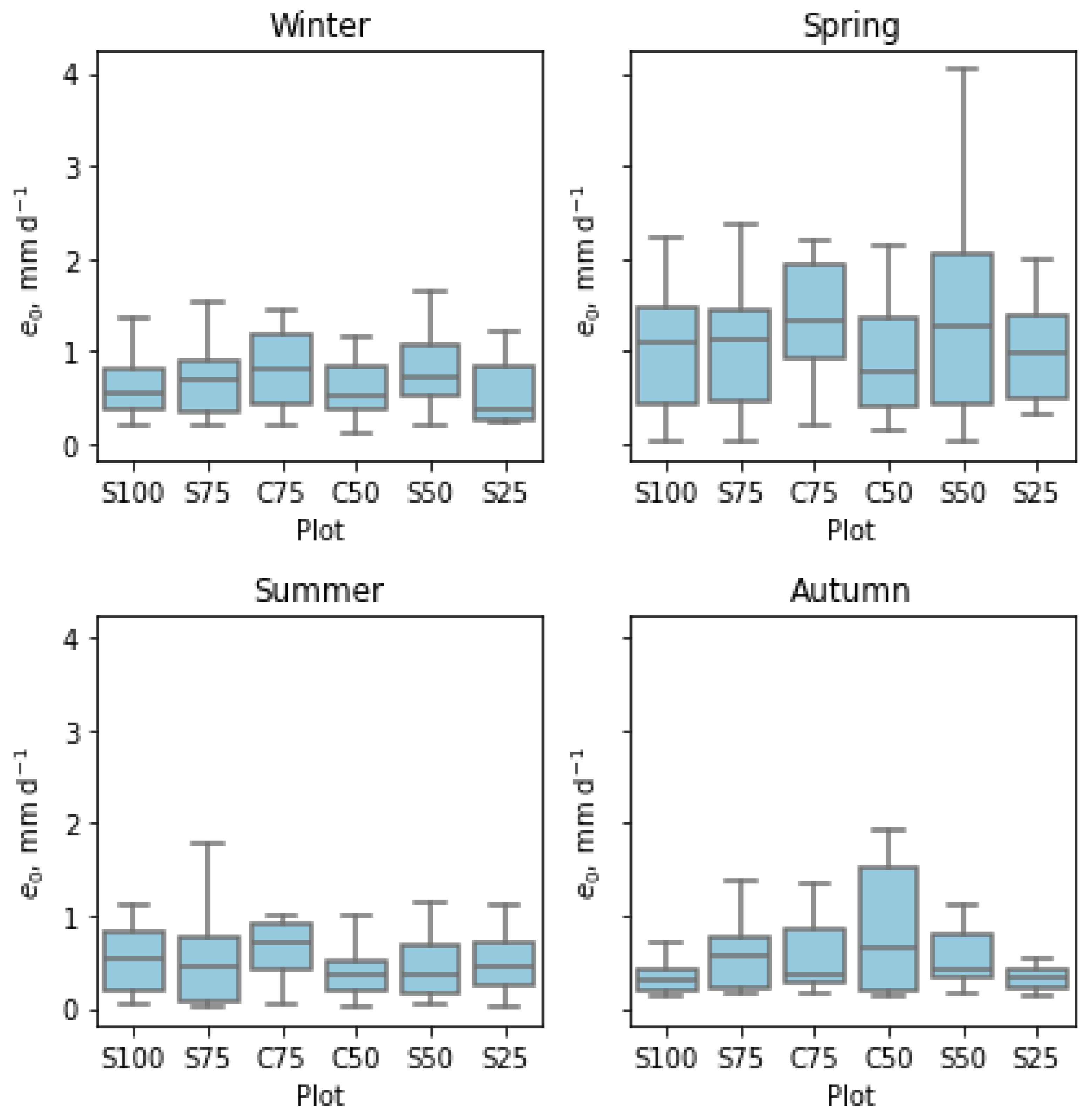
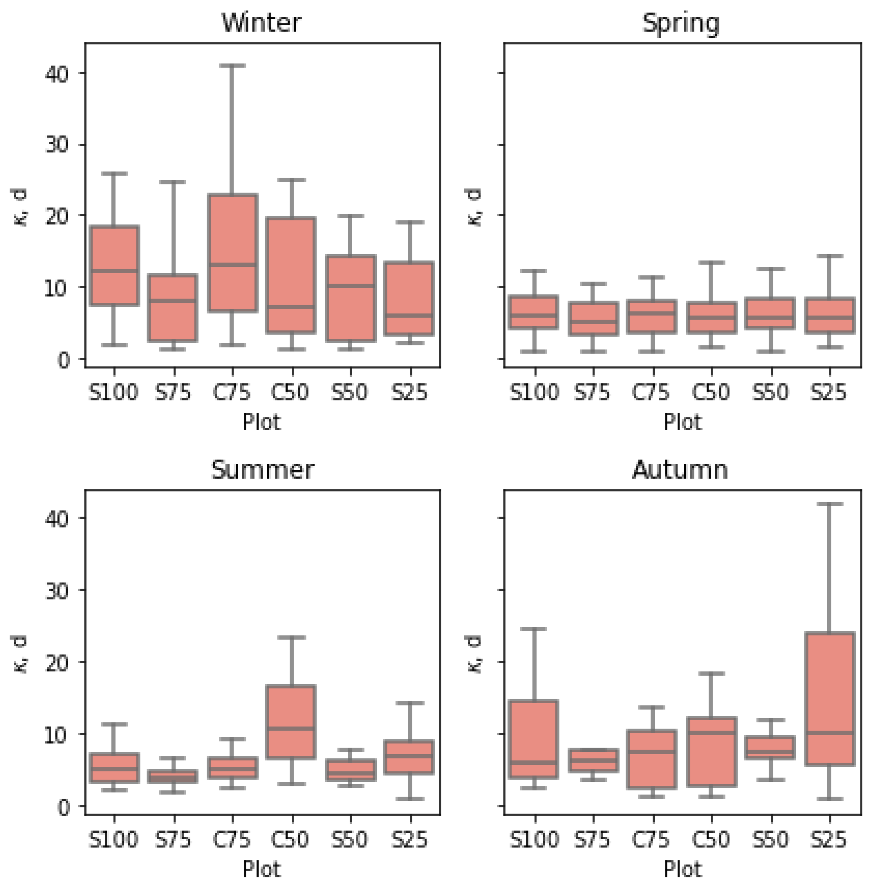
The box-and-whisker plots in Figure 6 and Figure 7 compare the estimated values of the parameters for each plot and season. In this stage, evaporation is controlled mainly by the soil; nevertheless, some differences are observed in the parameters depending on the season. In spring, the e0 values are higher than in other seasons and with different values between plots, while the values of κ are similar between plots and lower than in other seasons, indicating a faster evaporation process. In winter, the opposite happens; κ values are higher, which means a slower process and with variations between plots, while the reference evaporation, e0, is lower and without appreciable differences between plots.
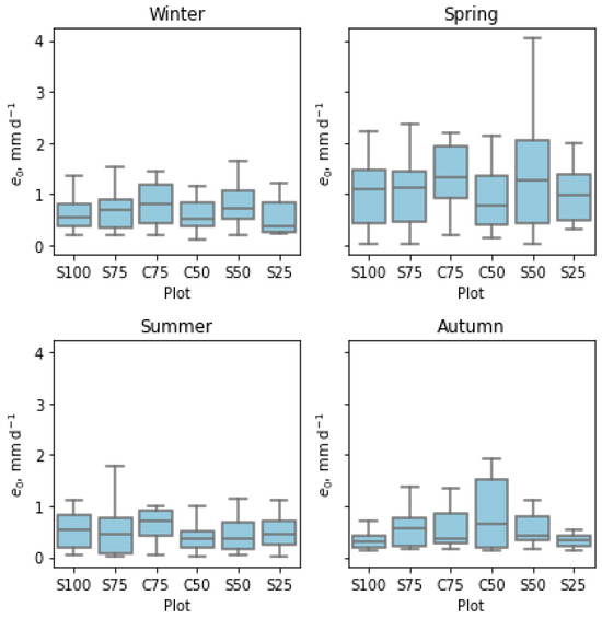
Figure 6.
Box-and-whisker plots representing the variation in the estimates for the Brutsaert reference evaporation rate (e0) differentiated by plot and season. The central horizontal bar in each rectangle represents the median value, the horizontal bars at the rectangles’ upper and lower boundaries are the values of the first (Q1) and third quartile (Q3), and the whiskers extend from the smallest to the largest values within 1.5 times the interquartile range (IQR), which is the range between the first quartile and third quartile.
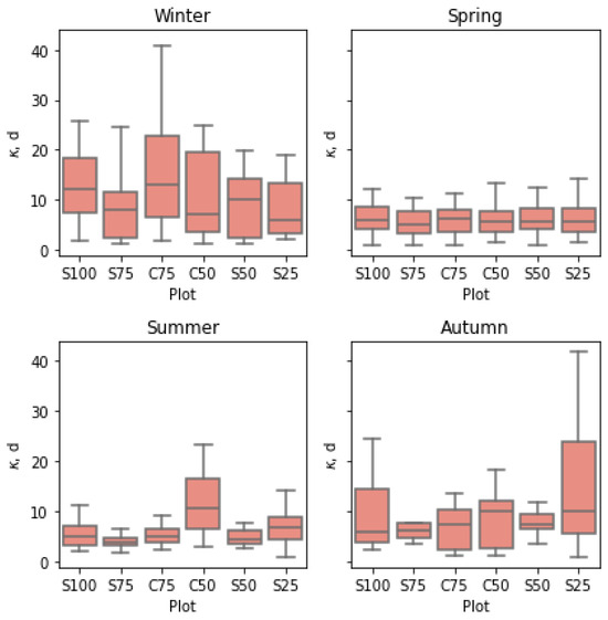
Figure 7.
Box-and-whisker plots representing the variation in the estimates for the Brutsaert reference time (κ) differentiated by plot and season. The central horizontal bar in each rectangle represents the median value, the horizontal bars at the rectangles’ upper and lower boundaries are the values of the first (Q1) and third quartile (Q3), and the whiskers extend from the smallest to the largest values within 1.5 times the interquartile range (IQR), which is the range between the first quartile and third quartile.
3.3. Relationship between Calculated Evaporation and Reference Evapotranspiration Rates
The relationship between the values of the parameter for the initial evaporation intensity in Brutsaert’s solution [47], , and the estimated reference evapotranspiration intensity based on meteorological information, e.g., [26], data provided by the respective observatories, , is depicted in Figure 8. In Figure 8b, a rising envelope trend is detected between the initial moisture, , at which the evaporation process begins, and the intensity of the process.
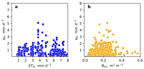
Figure 8.
Relationships of the reference evaporation rate by Brutsaert () with the reference evaporation from the agrometeorological station (ETo) (a), and with the initial substrate moisture at the onset of evaporation processes () (b), for the 6 plots of the green roofs in the selected drying periods.
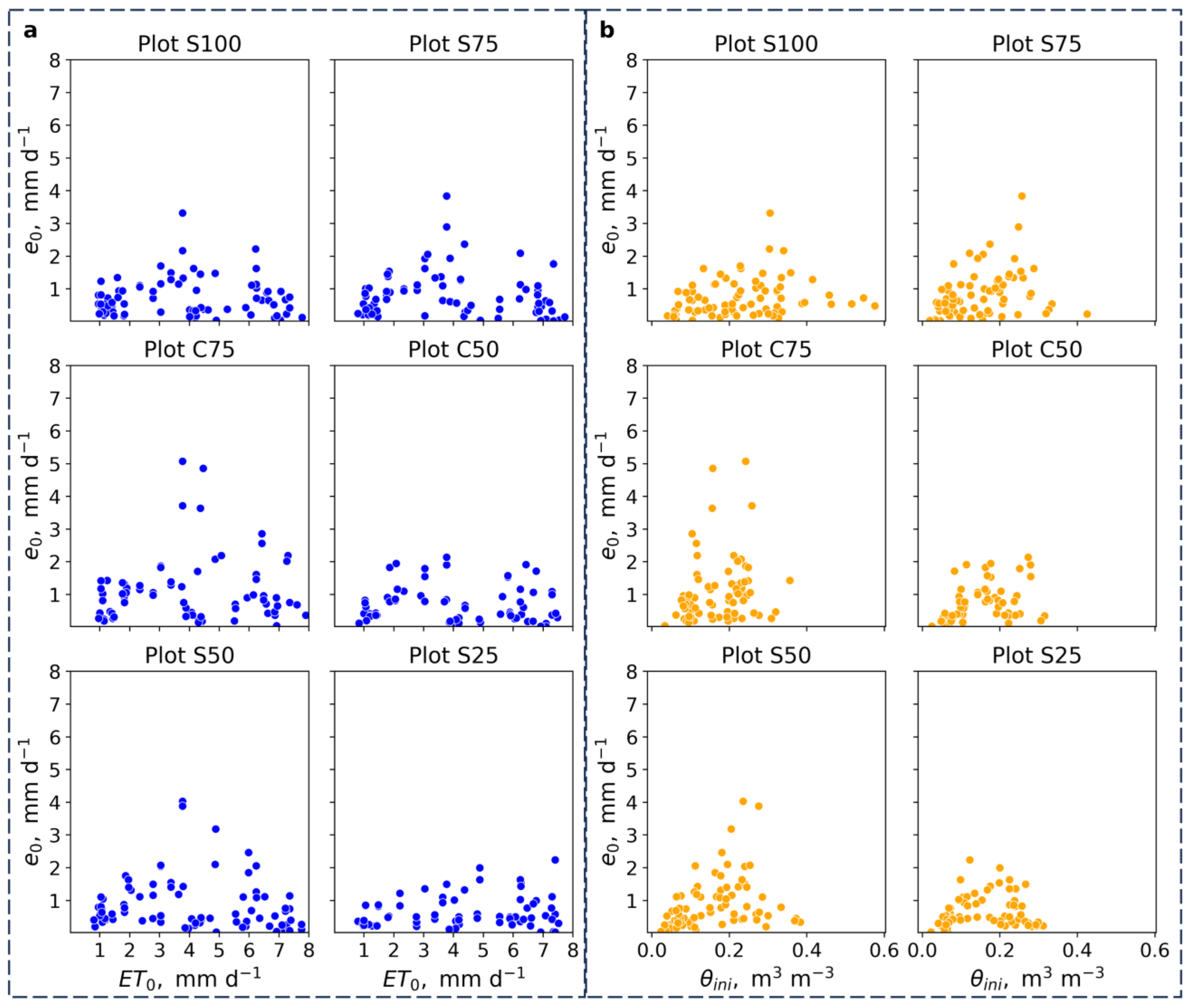
The same relationships have been explored for the drydowns corresponding to each plot (Figure 9) and each season (Figure 10). In Figure 9b, it can be observed that in the plots with a higher content of recycled aggregates, the average initial moisture during the drying periods is lower, and the maximum values reached are also lower. For instance, in plot S100, the initial moisture values () reach 0.6 m3/m3, whereas in plot S25, they only reach 0.3 m3/m3 (Figure 10b), indicating a lower water retention capacity.
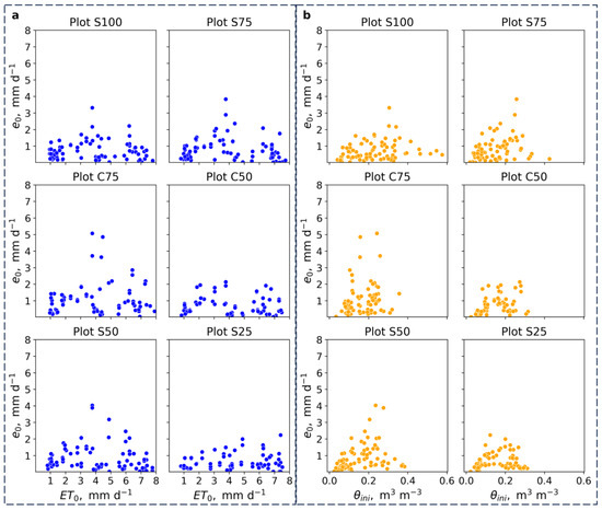
Figure 9.
Variation in each plot from the reference evaporation rate by Brutsaert () with (a) the computed potential evaporation rate from the agrometeorological station (ETo) and with (b) the initial substrate moisture at the onset of the evaporation processes ().
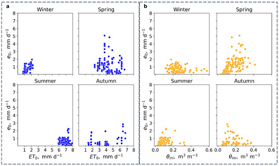
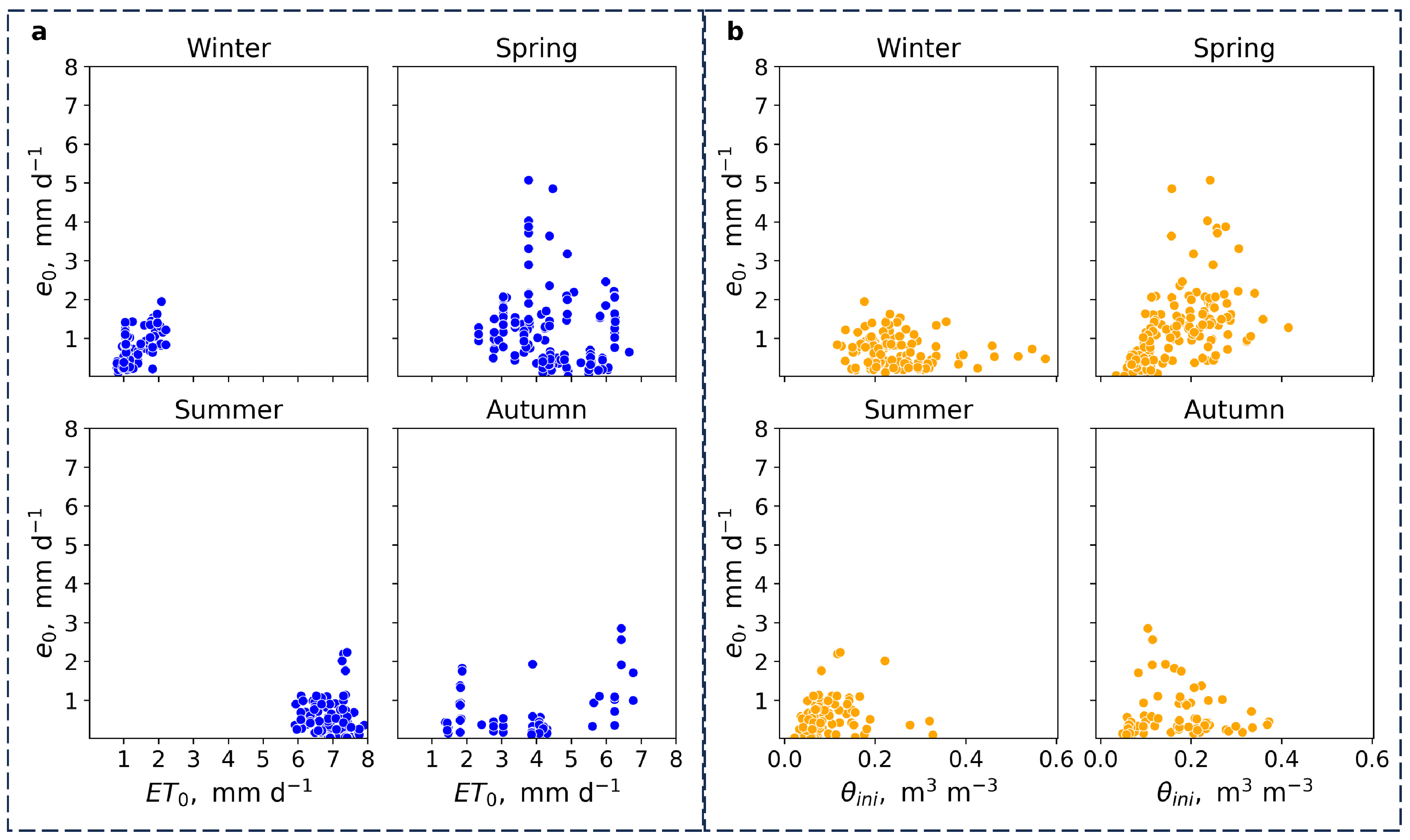
Figure 10.
Variation classified by season in the reference evaporation rate for the 6 plots with (a) the computed potential evaporation rate from the agrometeorological station (ETo), and with (b) the initial substrate moisture at the onset of the evaporation processes ().
In the different plots, no distinct patterns are found in the point clouds. However, for the different seasons, the point clouds are clustered in different sections of the graph. During winter and summer, the values are below approximately 2 mm d−1 in all plots, while in spring and autumn, there is greater dispersion of the data. This is due to both higher variability in and a broader range of variation, particularly in spring.
In any case, the estimated values of the initial evaporation rate are within the range of the reference evapotranspiration rates (ETos) measured in the nearby weather station.
3.4. Determination of Weighted-Mean Diffusivity
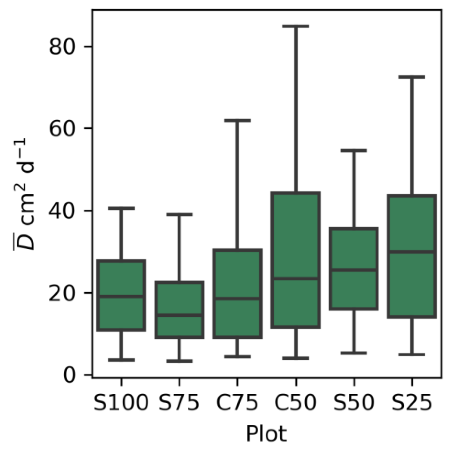
The values of the estimated weighted-mean diffusivity using Brutsaert’s equation [47], as defined by Equation (13), were obtained (Table 6 and Figure 11). The substrates of plots C50, S50, and S25, containing 50% and 75% recycled aggregates, stand out due to their higher mean and median values.
Table 6.
Mean, median, and standard deviation values of weighted-mean diffusivity () from Brutsaert’s [47] method.

Figure 11.
Box-and-whisker diagram of . The central horizontal bar in each rectangle represents the median value, the horizontal bars at the rectangles’ upper and lower boundaries are the values of the first (Q1) and third quartile (Q3), and the whiskers extend from the smallest to the largest values within 1.5 times the interquartile range (IQR), which is the range between the first quartile and third quartile.
Looking at the substrate mixtures with substrate S, there is an increase in with the increase in RAs, except for in plot S100, which has no RAs. Looking at the substrate mixtures containing substrate C, the same increasing trend in with RA content is found. This trend is coherent with a coarser texture as RA content increases. These values are not too far from the order of magnitude of the field observations reported by Brutsaert [47].
The variability of values obtained for the weighted-mean diffusivity are due to the variable limits between the initial and final moisture content of these substrates during drydown periods, and to the inherent variability of them.
The different behavior of plot S100 could be attributed to the high percentage of total carbon in the substrate. The percentage of total carbon in the different substrates was measured in the substrates in 2018, obtaining for mixtures with vegetative substrate S a 16.6% weight of total carbon in plot S100, a 3.8% in S75, a 2.6% in S50, and a 1.9% in S25. And for mixtures with substrate C, these values were a 4.5% in plot C75 and a 2.6% in C50. Therefore, for both vegetative substrates (S and C), there was a decreasing trend in carbon content with the increase in recycled aggregates.
It is evident that S100 has an exceptionally high amount of organic matter, which could alter diffusivity values. The presence of organic matter can improve soil structure and porosity, thereby increasing diffusivity.
To statistically check if the obtained sets of weighted-mean diffusivity values in the six plots have the same mean value, a Kruskal and Wallis test was applied (Section 2.8). The null hypothesis that all the sets have the same mean was tested, and the value obtained for the statistic T was T = 35.2. With 5 degrees of freedom, this yielded a probability of p = 0.0001. Therefore, the null hypothesis was rejected, confirming that there are appreciable differences between the substrates, as the weighted-mean diffusivity values suggested.
A closer comparison can be made between the substrates; the datasets obtained from each sensor were compared pairwise with the Mann–Whitney test. Table 7 shows the probabilities of the statistic T of Mann–Whitney for all the combinations of the substrates.
Table 7.
Probability of the Mann–Whitney statistic for the comparison between the mean values of the weighted-mean diffusivity values of the substrates. The values smaller than 0.025 indicate that there are relevant differences among the respective substrates.
Due to the natural compaction of the porous media and the potential clogging of pores by dust particles, the weighted-mean diffusivity exhibits a gradual decrease over time at a relatively low rate, even within a 6-year period. Nevertheless, this effect does not impact the results presented in this study.
3.5. Estimation of the Saturated Hydraulic Conductivity
As an additional result, the two different methods adopted for the estimation of mean-weighted water diffusivity—the Brutsaert method during the evaporation process and the van Genuchten–Mualem water retention and hydraulic conductivity function—enable the estimation of the saturated hydraulic conductivity.
However, this procedure requires that the initial moisture content at the start of the evaporation process is not too low to avoid very small values in the denominator of Equation 20. Otherwise, the estimation of hydraulic conductivity would be unreasonably high and therefore unreliable. The estimated saturated hydraulic conductivity using Equation 20 is variable within each substrate, though differences are evident among the substrates, as outlined in Table 8, Figure 12, and the box-and-whisker plot in Figure 13.
Table 8.
Values of the estimated saturated hydraulic conductivity () for each substrate, obtained using the method by Brutsaert [47].
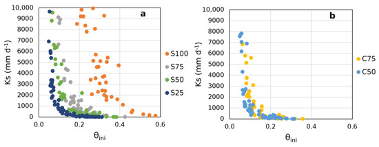
Figure 12.
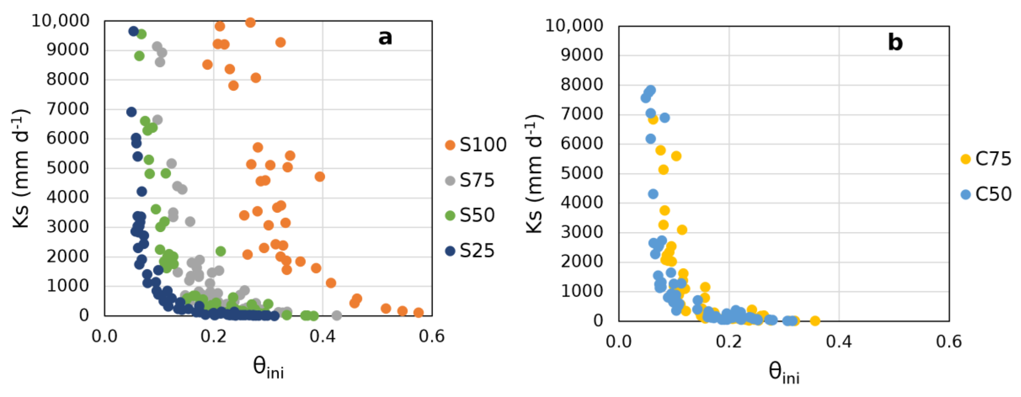
Variations in Ks with the initial moisture of each drydown period (a) for the mixtures with vegetative substrate type S, and (b) for the mixtures with vegetative substrate type C.

Figure 13.
Box-and-whisker plot of the saturated hydraulic conductivity, . The central horizontal bar in each rectangle represents the median value, the horizontal bars at the rectangles’ upper and lower boundaries are the values of the first (Q1) and third quartile (Q3), and the whiskers extend from the smallest to the largest values within 1.5 times the interquartile range (IQR), which is the range between the first quartile and third quartile.
The maximum mean value of hydraulic conductivity corresponds to substrate S100, followed by substrates S75 and S50. In plots S100, S75, S50, and S25, with the same vegetative substrate and increasing percentage of recycled aggregates, a general trend in decreasing saturated hydraulic conductivity, ks, with an increase in the percentage of aggregates is observed. The opposite pattern is observed in plots C75 and C50, where aggregates are mixed with compost (Table 1), with a 313 cmd−1 difference in the median value.
The values of saturated hydraulic conductivity fall within the range reported by various groups, such as Timlin et al. [70], Chapuis [71], Assouline and Or [72], and Wang et al. [73], among others. Although direct measurement methods, as suggested by Stanic et al. [74], are more reliable and not particularly difficult, studies such as that by Zhang and Schaap [75] highlight that they are expensive and sometimes not feasible. This methodology offers an alternative to pedotransfer functions for the estimation of .
These results enable a straightforward characterization of certain hydrophysical properties of green roof substrates, particularly in Mediterranean climates where long drydown periods are frequent. Although this modelling exercise does not directly serve to predict substrate moisture, it provides estimates of the soil properties and , which can be useful in physical models to help estimate substrate moisture.
One possible limitation that could explain some of the observed variability is that the influence of vegetation was considered in this study. For future studies, it may be necessary to separate evaporation from transpiration, possibly with the assistance of the leaf area index. An influence on the analysis is also expected from external conditions such as temperature. Higher temperatures generally increase the kinetic energy of molecules, enhancing diffusivity, while lower temperatures slow down molecular movement, decreasing diffusivity.
4. Conclusions
The substrates used in green roofs, being porous media, despite their slight thickness can be described using the same physical principles that apply to other porous media. This study demonstrates the possibility of characterizing two key hydraulic properties of green roof substrates in a straightforward manner.
The regression analysis of Brutsaert’s [47] exponential evaporation equation allows for the evaluation of the hydraulic diffusivity of the substrates. Although Brutsaert originally developed this equation in 2014, this study emphasizes its suitability for characterizing green roof substrates. Moreover, by estimating the weighted-mean diffusivity () from the substrate retention curve, the value of the saturated hydraulic conductivity () can be determined. This approach is particularly well suited for Mediterranean climates, where drying periods can easily be identified without interference from precipitation. This study marks the first application of this method to green roofs, demonstrating it to be both highly efficient and straightforward.
The results for and for each plot show variability due to the heterogeneity of the substrates, the initial moisture content during drydown periods, and external influences. The median values on the plots range from 14.5 to 29.9 cm2d−1 for , and from 22 to 361 cmd−1 for . These values are within the ranges reported by other research groups. Generally, in the analyzed green roofs, an increase in and a decrease in are observed as the percentage of recycled aggregates in the substrates increases.
The results support the adoption of analytical solutions from the Richards equation to characterize hydrological properties in green roofs during drying periods. However, there are still some challenges to address, specifically, improving the analysis of processes in a thin substrate layer covering a large surface area and accounting for vegetation and environmental factors like solar radiation and wind, among others.
Author Contributions
Conceptualization, J.V.G., A.M.L. and T.V.; methodology, B.C.-A., J.V.G. and A.M.L.; software, B.C.-A. and J.V.G.; validation, G.M. and B.C.-A.; formal analysis, B.C.-A., J.V.G. and A.M.L.; investigation, B.C.-A. and A.H.; resources, J.V.G. and T.V.; data curation, B.C.-A.; writing—original draft preparation, B.C.-A.; writing—review and editing, A.M.L., J.V.G., T.V., A.P. and Á.L; visualization, B.C.-A.; supervision, J.V.G.; project administration, T.V. and G.M.; funding acquisition, T.V., A.P., Á.L., A.M.L., and J.V.G. All authors have read and agreed to the published version of the manuscript.
Funding
This research was funded by (1) the European Regional Development Fund (ERDF) and Consejería de Fomento y Vivienda de la Agencia de Obra Pública de la Junta de Andalucía, through grant number GGI3003IDIB, with the project “Optimizing the Green roof potential for the energetic rehabilitation of buildings: interaction between recycled materials, hydraulic properties and energetic efficiency”, and later by (2) FEDER Operative program Andalucía 2014–2020 and Consejería de Economía y Conocimiento de la Junta de Andalucía, through grant number 1381322-R, with the project “NATVR—New advances in green roofs towards the regeneration of urban ecosystems”.
Data Availability Statement
The raw data supporting the conclusions of this article will be made available by the authors on request.
Conflicts of Interest
The authors declare no conflicts of interest. The funders had no role in the design of the study; in the collection, analyses, or interpretation of data; in the writing of the manuscript; or in the decision to publish the results.
References
- Jacobs, S.J.; Gallant, A.J.E.; Tapper, N.J. Use of cool roofs and vegetation to mitigate urban heat and improve human thermal stress in Melbourne, Australia. J. Appl. Meteorol. Climatol. 2018, 57, 1747–1764. [Google Scholar] [CrossRef]
- Alim, M.A.; Rahman, A.; Tao, Z.; Gardner, B.; Griffith, R.; Liebman, M. Green roof as an effective tool for sustainable urban development: An Australian perspective in relation to stormwater and building energy management. J. Clean. Prod. 2022, 362, 13261. [Google Scholar] [CrossRef]
- Hashemi, S.S.G.; Mahmud, H.B.; Ashraf, M.A. Performance of green roofs with respect to water quality and reduction of energy consumption in tropics: A review. Renew. Sustain. Energy Rev. 2015, 52, 669–679. [Google Scholar] [CrossRef]
- Mihalakakou, G.; Souliotis, M.; Papadaki, M.; Menounou, P.; Dimopoulos, P.; Kolokotsa, D.; Paravantis, J.A.; Tsangrassoulis, A.; Panaras, G.; Giannakopoulos, E.; et al. Green roofs as a nature-based solution for improving urban sustainability: Progress and perspectives. Ren. Sustain. Energy Rev. 2023, 180, 113306. [Google Scholar] [CrossRef]
- Santamouris, M. Cooling the cities—A review of reflective and green roof mitigation technologies to fight heat island and improve comfort in urban environments. Sol. Energy 2014, 103, 682–703. [Google Scholar] [CrossRef]
- Coutts, A.M.; Daly, E.; Beringer, J.; Tapper, N.J. Assessing practical measures to reduce urban heat: Green and cool roofs. Build. Eng. 2013, 70, 260–275. [Google Scholar] [CrossRef]
- van Renterghem, T.; Hornikx, M.; Forssen, J.; Botteldooren, D. The potential of building envelope greening to achieve quietness. Build. Environ. 2013, 51, 34–44. [Google Scholar] [CrossRef]
- Berndtsson, J.C. Green roof performance towards management of runoff water quantity and quality: A review. Ecol. Eng. 2010, 36, 351–360. [Google Scholar] [CrossRef]
- Berndtsson, J.C.; Emilsson, T.; Bengtsson, L. The influence of extensive vegetated roofs on runoff water quality. Sci. Total Environ. 2006, 355, 48–63. [Google Scholar] [CrossRef]
- Gnecco, I.; Palla, A.; Lanza, L.G.; La Barbera, P. The Role of Green Roofs as a Source/sink of Pollutants in Storm Water Outflows. Water Resour. Manag. 2013, 27, 4715–4730. [Google Scholar] [CrossRef]
- Stovin, V.; Vesuviano, G.; De-Ville, S. Defining green roof detention performance. Urban Water J. 2017, 14, 574–588. [Google Scholar] [CrossRef]
- Mentens, J.; Raes, D.; Hermy, M. Green roofs as a tool for solving the rainwater runoff problem in the urbanized 21st century? Landsc. Urban Plan. 2006, 77, 217–226. [Google Scholar] [CrossRef]
- Lamera, C.; Becciu, G.; Rulli, M.C.; Rosso, R. Green roofs effects on the urban water cycle components. Procedia Eng. 2014, 70, 988–997. [Google Scholar] [CrossRef]
- Hui, S.C.M.; Chu, C.H.T. Green roofs for stormwater mitigation in Hong Kong. In Proceedings of the Joint Symposium 2009: Design for Sustainable Performance, Hong Kong, 25 November 2009. [Google Scholar]
- McColl, K.A.; Wang, W.; Peng, B.; Akbar, R.; Short Gianotti, D.J.; Lu, H.; Pan, M.; Entekhabi, D. Global characterization of surface soil moisture drydowns. Geophys. Res. Lett. 2017, 44, 3682–3690. [Google Scholar] [CrossRef]
- Lucatelli, L.; Mark, O.; Mikkelsen, P.S.; Arnbjerg-Nielsen, K.; Jensen, M.B.; Binning, P.J. Modelling of green roof hydrological performance for urban drainage applications. J. Hydrol. 2014, 519, 3237–3248. [Google Scholar] [CrossRef]
- Vesuviano, G.; Sonnenvald, F.; Stovin, V. A two-stage storage routing model for green roof runoff detention. Novatech 2013, 69, 1191–1197. [Google Scholar] [CrossRef]
- Carson, T.; Keeley, M.; Marasco, D.E.; McGillis, N.; Culligan, P. Assessing methods for predicting green roof rainfall capture: A comparison between full-scale observations and four hydrologic models. Urban Water J. 2017, 14, 589–603. [Google Scholar] [CrossRef]
- Castro, A.S.; Goldenfundum, A.; da Silveira, A.L.; DallAgnol, A.L.B.; Loebens, L.; Demarco, C.F.; Leandro, D.; Nadaleti, W.C.; Quadro, M.S. The analysis of green roof’s runoff volumes and its water quality in an experimental study in Porto Alegre, Southern Brazil. Environ. Sci. Pollut. Res. 2020, 27, 9520–9534. [Google Scholar] [CrossRef] [PubMed]
- Kemp, S.; Hadley, P.; Blanusa, T. The influence of plant type on green roof rainfall retention. Urban Ecosyst. 2019, 22, 355–366. [Google Scholar] [CrossRef]
- She, N.; Pang, J. Physically based green roof model. J. Hydrol. Eng. 2010, 15, 458–466. [Google Scholar] [CrossRef]
- Green, W.H.; Ampt, G.A. Studies on Soil Physics, 1: The Flow of Air and Water through Soils. J. Agric. Sci. 1911, 4, 1–24. [Google Scholar] [CrossRef]
- Cascone, S.; Coma, J.; Gagliano, A.; Pérez, G. The evapotranspiration process in green roofs: A review. Build. Environ. 2019, 147, 337–355. [Google Scholar] [CrossRef]
- Ebrahimian, A.; Wadzuk, B.; Traver, R. Evapotranspiration in green stormwater infrastructure systems. Sci. Total Environ. 2019, 688, 797–810. [Google Scholar] [CrossRef]
- Starry, O.; Lea-Cox, J.; Rivstey, A.; Cohan, S. Parameterizing a water-balance model for predicting stormwater runoff from green roofs. J. Hydrol. Eng. 2016, 21, 04016046. [Google Scholar] [CrossRef]
- Allen, R.G.; Pereira, L.S.; Raes, D.; Smith, M. Crop Evapotranspiration—Guidelines for Computing Crop Water Requirements—Fao Irrigation and Drainage Paper 56; FAO: Roma, Italy, 1988. [Google Scholar]
- Stovin, V.; Poë, S.; Berretta, C. A modelling study of long-term Green roof retention performance. J. Environ. Manag. 2013, 131, 206–215. [Google Scholar] [CrossRef] [PubMed]
- Berretta, C.; Poë, S.; Stovin, V. Moisture content behaviour in extensive green roofs during dry periods: The influence of vegetation and substrate characteristics. J. Hydrol. 2014, 511, 374–386. [Google Scholar] [CrossRef]
- Brutsaert, W. Hydrology: An Introduction; Cambridge University Press: Cambridge, UK, 2005. [Google Scholar]
- Alley, W.M. On the treatment of evapotranspiration, soil moisture accounting, and aquifer recharge in monthly water balance models. Water Resour. Res. 1984, 20, 1137–1149. [Google Scholar] [CrossRef]
- Gardner, W.R. Solutions of the flow equation for the drying of soils and other porous media. Soil Sci. Soc. Am. Proc. 1959, 23, 183–187. [Google Scholar] [CrossRef]
- Hilten, R.W.; Lawrence, T.M.; Tollner, E.W. Modeling stormwater runoff from green roofs with HYDRUS-1D. J. Hydrol. 2008, 358, 288–293. [Google Scholar] [CrossRef]
- Sandoval, V.; Bonilla, C.A.; Gironás, J.; Vera, S.; Victorero, F.; Bustamante, W.; Rojas, V.; Leiva, E.; Pastén, P.; Suárez, F. Porous media characterization to simulate water and heat transport through green roof substrates. Vadose Zone J. 2017, 16, 1–14. [Google Scholar] [CrossRef]
- Carbone, M.; Garofalo, G.; Nigro, C.; Piro, P. A conceptual model for predicting hydraulic behavior of a green roof. Procedia Eng. 2014, 70, 266–274. [Google Scholar] [CrossRef]
- Kader, S.; Chadalavada, S.; Jaufer, L.; Spalevic, V.; Dudic, B. Green roofs substrates—A literature review. Fronts Build. Environ. 2022, 8, 1019362. [Google Scholar] [CrossRef]
- Liu, R.; Fassman-Beck, E. Effect of composition on basic properties of engineered media for living roofs and bioretention. J. Hydrol. Eng. 2016, 21, 06016002. [Google Scholar] [CrossRef]
- Peng, Z.; Smith, C.; Stovin, V. The importance of unsaturated hydraulic conductivity measurements for green roof detention modelling. J. Hydrol. 2020, 590, 125273. [Google Scholar] [CrossRef]
- Fassman-Beck, E.; Voyde, E.; Simcock, R.; Hong, Y.S. 4 Living roofs in 3 locations: Does configuration affect runoff mitigation? J. Hydrol. 2013, 490, 11–20. [Google Scholar] [CrossRef]
- Kader, S.; Spalevic, V.; Dudic, B. Feasibility study for estimating optimal substrate parameters for sustainable green roof in Sri Lanka. Environ. Dev. Sustain. 2022, 26, 2507–2533. [Google Scholar] [CrossRef]
- Coelho, K.; Almeida, J.; Castro, F.; Ribeiro, A.; Teixeira, T.; Palha, P.; Simões, N. Experimental characterization of different ecological substrates for use in green roof systems. Sustainability 2022, 15, 575. [Google Scholar] [CrossRef]
- Sloan, J.J.; Ampim, P.A.; Basta, N.T.; Scott, R. Addressing the need for soil blends and amendments for the highly modified urban landscape. Soil Sci. Soc. Am. J. 2012, 76, 1133–1141. [Google Scholar] [CrossRef]
- López-Uceda, A.; Galvín, A.P.; Ayuso, J.; Jiménez, J.R.; Vanwallaghem, T.; Peña, A. Risk assessment by percolation leaching tests of extensive green roofs with fine fraction of mixed recycled aggregates from construction and demolition waste. Environ. Sci. Pollut. Res. 2018, 25, 36024–36034. [Google Scholar] [CrossRef]
- Laio, F.; Porporato, A.; Ridolfi, L.; Rodríguez-Iturbe, I. Plants in water-controlled ecosystems: Active role in hydrological processes and response to water stress: II. Probabilistic soil moisture dynamics. Adv. Water Resour. 2001, 24, 707–723. [Google Scholar] [CrossRef]
- Or, D.; Lehmann, P.; Sharhaeeni, E.; Shokri, N. Advances in soil evaporation physics—A review. Vadose Zone J. 2013, 12, 1–16. [Google Scholar] [CrossRef]
- Koster, R.D.; Suarez, M.J. Soil moisture memory in climate models. J. Hydrometeorol. 2001, 2, 558–570. [Google Scholar] [CrossRef]
- Poë, S.; Stovin, V.; Berretta, C. Parameters influencing the regeneration of a green roof’s retention capacity via evapotranspiration. J. Hydrol. 2015, 523, 356–367. [Google Scholar] [CrossRef]
- Brutsaert, W. Daily evaporation from drying soil: Universal parameterization with similarity. Water Resour. Res. 2014, 50, 3206–3215. [Google Scholar] [CrossRef]
- Brutsaert, W. The daily mean zero-flux plane during soil-controlled evaporation: A Green’s function approach. Water Resour. Res. 2014, 50, 9405–9413. [Google Scholar] [CrossRef]
- Crank, J. The Mathematics of Diffusion, 2nd ed.; Oxford University Press: London, UK, 1975. [Google Scholar]
- van Genuchten, M.T. A Closed-form Equation for Predicting the Hydraulic Conductivity of Unsaturated Soils. Soil Sci. Soc. Am. J. 1980, 44, 892–898. [Google Scholar] [CrossRef]
- Peel, M.C.; Finlayson, B.L.; McMahon, T.A. Updated world map of the Köppen-Geiger climate classification. Hydrol. Earth Syst. Sci. 2007, 11, 1633–1644. [Google Scholar] [CrossRef]
- Villalobos, F.J.; Testi, L.; Estaciones Agrometeorológicas. Universidad de Córdoba. Available online: https://www.uco.es/grupos/meteo/ (accessed on 2 August 2024).
- Google Earth V 7.3.3.7786. Image of Cordoba University Green Roofs, Córdoba, Spain, 29 October 2017. Available online: https://earth.google.com/web/ (accessed on 26 November 2020).
- Grossman, R.B.; Reinsch, T.G. Bulk density and linear extensibility. In Methods of Soil Analysis: Part 4. Physical Methods; Dane, J.H., Clarke, G.C., Eds.; SSSA Book Series no. 5; Soil Science Society of America: Madison, WI, USA, 2002. [Google Scholar]
- Caneva, G.; Kumbaric, A.; Savo, V.; Casalini, R. Ecological approach in selecting extensive green roof plants: A data-set of Mediterranean plants. Plant Biosyst. 2013, 149, 374–383. [Google Scholar] [CrossRef]
- Campbell Scientific, Inc. CS616 and CS625 Water Content Reflectometers, Instruction Manual Revision: 6/15; Campbell Scientific, Inc.: Logan, UT, USA, 2002; 46p. [Google Scholar]
- Dane, J.H.; Hopmans, J.W. Laboratory methods. In Methods in Soil Analysis: Part 4. Physical Methods; Dane, J.H., Topp, G.C., Eds.; Book series no. 5; Soil Science Society of America: Madison, WI, USA, 2002; pp. 67–720. [Google Scholar]
- Montes, C. Determinación de la Curva de Retención de Agua de Diferentes Sustratos Para Techos Verdes. Master’s Thesis, Universidad de Córdoba, Córdoba, Spain, 2020. [Google Scholar]
- Virtanen, P.; Gommers, R.; Oliphant, T.E.; Haberland, M.; Reddy, T.; Cournapeau, D.; van der Walt, S.J. SciPy 1.0: Fundamental Algorithms for Scientific Computing in Python. Nat. Methods 2020, 17, 261–272. [Google Scholar] [CrossRef]
- Moré, J.J. The Levenberg-Marquardt algorithm: Implementation and theory. In Numerical Analysis; Springer: Heidelberg/Berlin, Germany, 1978; pp. 105–116. [Google Scholar] [CrossRef]
- Raats, P.A.C.; Knight, H.H. The contributions of lewis Fry Richardson to drainage theory, soil physics, and the soil-plat-atmosphere continuum. Fronts Environ. Sci. 2018, 6, 13. [Google Scholar] [CrossRef]
- Gardner, W.R.; Mayhug, M.S. Solutions and tests of the diffusion equation for the movement of water in soil. Soil Sci. Soc. Am. Proc. 1958, 22, 197–201. [Google Scholar] [CrossRef]
- Brutsaert, W. The unit response of groundwater outflow from a hillslope. Water Resour. Res. 1994, 30, 2759–2763. [Google Scholar] [CrossRef]
- Wilks, D.S. Statistical Methods in the Atmospheric Sciences, 3rd ed.; Elsevier: Amsterdam, The Netherlands, 2011. [Google Scholar]
- Kutilek, M.; Nielsen, D.R. Soil Hydrology; Catena Verlag: Cremlingen-Dersted, Germany, 1994. [Google Scholar]
- Villareal, R.; Soracco, C.G.; Lozano, L.A.; Melani, E.M.; Sarli, G.O. Diffusivity and sorptivity determination at different soil water contents from horizontal infiltration. Geoderma 2019, 338, 88–96. [Google Scholar] [CrossRef]
- Abramowitz, M.; Stegun, I.D. Handbook of Mathematical Functions; Dover Publications: Mineola, NY, USA, 1964. [Google Scholar]
- Press, W.H.; Teikolsky, S.A.; Vetterling, W.T.; Flannery, B.P. Numerical Recipes: The Art of Scientific Computing, 2nd ed.; Cambridge University Press: Cambridge, UK, 1992. [Google Scholar]
- Conover, W.J. Practical Nonparametric Statistics, 2nd ed.; John Wiley and Sons: New York, NY, USA, 1980. [Google Scholar]
- Timlin, D.J.; Ahuja, L.R.; Pachepsky, Y.; Williams, R.D.; Giménez, D.; Rawls, W. Use of Brooks-Corey from parameters to improve estimates of saturated conductivity effective porosity. Soil Sci. Soc. Am. J. 1999, 63, 1086–10692. [Google Scholar] [CrossRef]
- Chapuis, R.P. Predicting the saturated hydraulic conductivity of soils: A review. Bull. Eng. Geol. Environ. 2012, 71, 401–434. [Google Scholar] [CrossRef]
- Assouline, S.; Or, D. Conceptual and parametric representation of soil hydraulic properties: A review. Vadose Zone J. 2013, 12, vzj2013.07.0121. [Google Scholar] [CrossRef]
- Wang, J.P.; Francois, B.; Lambert, P. Equations for hydraulic conductivity estimation from particle size distribution: A dimensional analysis. Water Resour. Res. 2017, 53, 8127–8134. [Google Scholar] [CrossRef]
- Stanić, F.; Cui, Y.J.; Delage, P.; de Laure, E.; Versini, P.A.; Schertzer, D.; Tchiguirinskaia, I. A device for the simultaneous determination of the water retention properties and the hydraulic conductivity function of an unsaturated coarse material; Application to a green-roof volcanic substrate. Geotech. Test. J. 2020, 43, 547–564. [Google Scholar] [CrossRef]
- Zhang, Y.; Schaap, M.G. Estimation of saturated hydraulic conductivity with pedotransfer functions: A review. J. Hydrol. 2019, 575, 1011–1030. [Google Scholar] [CrossRef]


Disclaimer/Publisher’s Note: The statements, opinions and data contained in all publications are solely those of the individual author(s) and contributor(s) and not of MDPI and/or the editor(s). MDPI and/or the editor(s) disclaim responsibility for any injury to people or property resulting from any ideas, methods, instructions or products referred to in the content. |
© 2024 by the authors. Licensee MDPI, Basel, Switzerland. This article is an open access article distributed under the terms and conditions of the Creative Commons Attribution (CC BY) license (https://creativecommons.org/licenses/by/4.0/).