
Integrated Basin-Scale Modelling for Sustainable Water Management Using MIKE HYDRO Basin Model: A Case Study of Parvati Basin, India

 ,
,  ,
,  ,
,  ,
, 
Abstract
1. Introduction
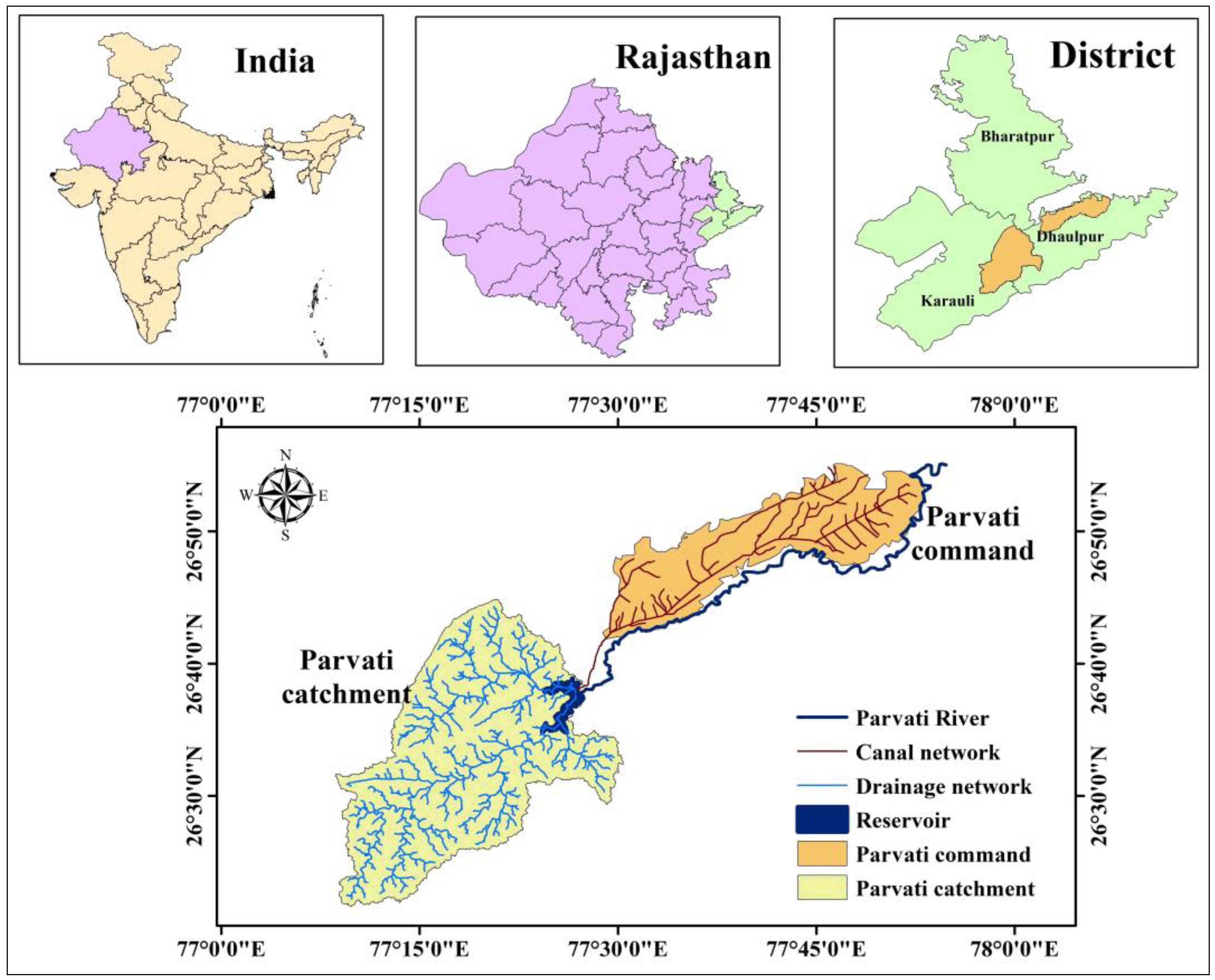
2. Study Area
Parvati Basin
3. Methodology
3.1. Data Products Used in the Study
3.2. Rainfall–Runoff Modelling
3.3. Water Demand and Supply Analysis
3.4. Scenarios Development
3.5. Performance Indicators
4. Results and Discussion
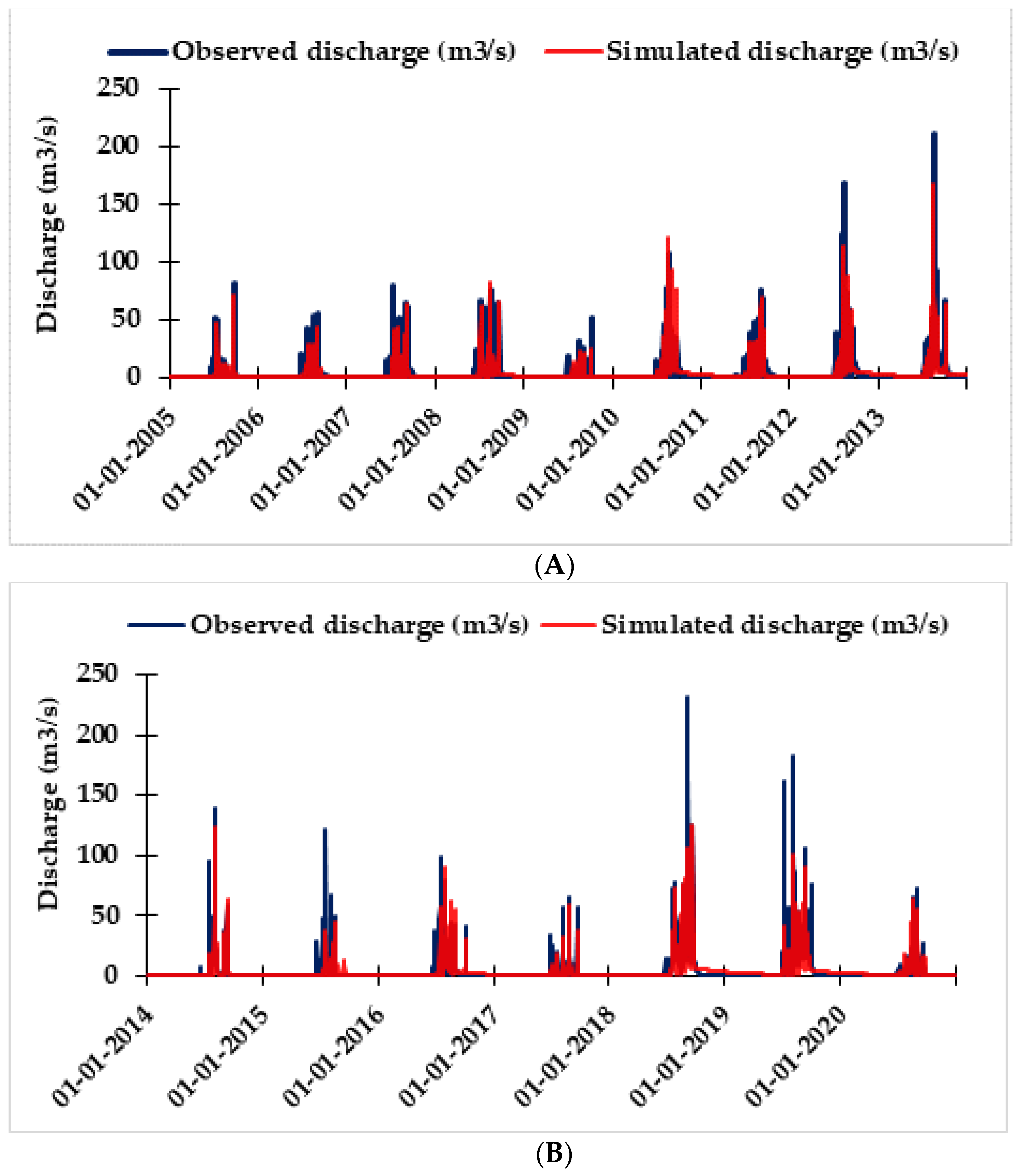
4.1. MIKE11 NAM Model Setup
4.2. Water Management Model for Demand and Deficit Assessment
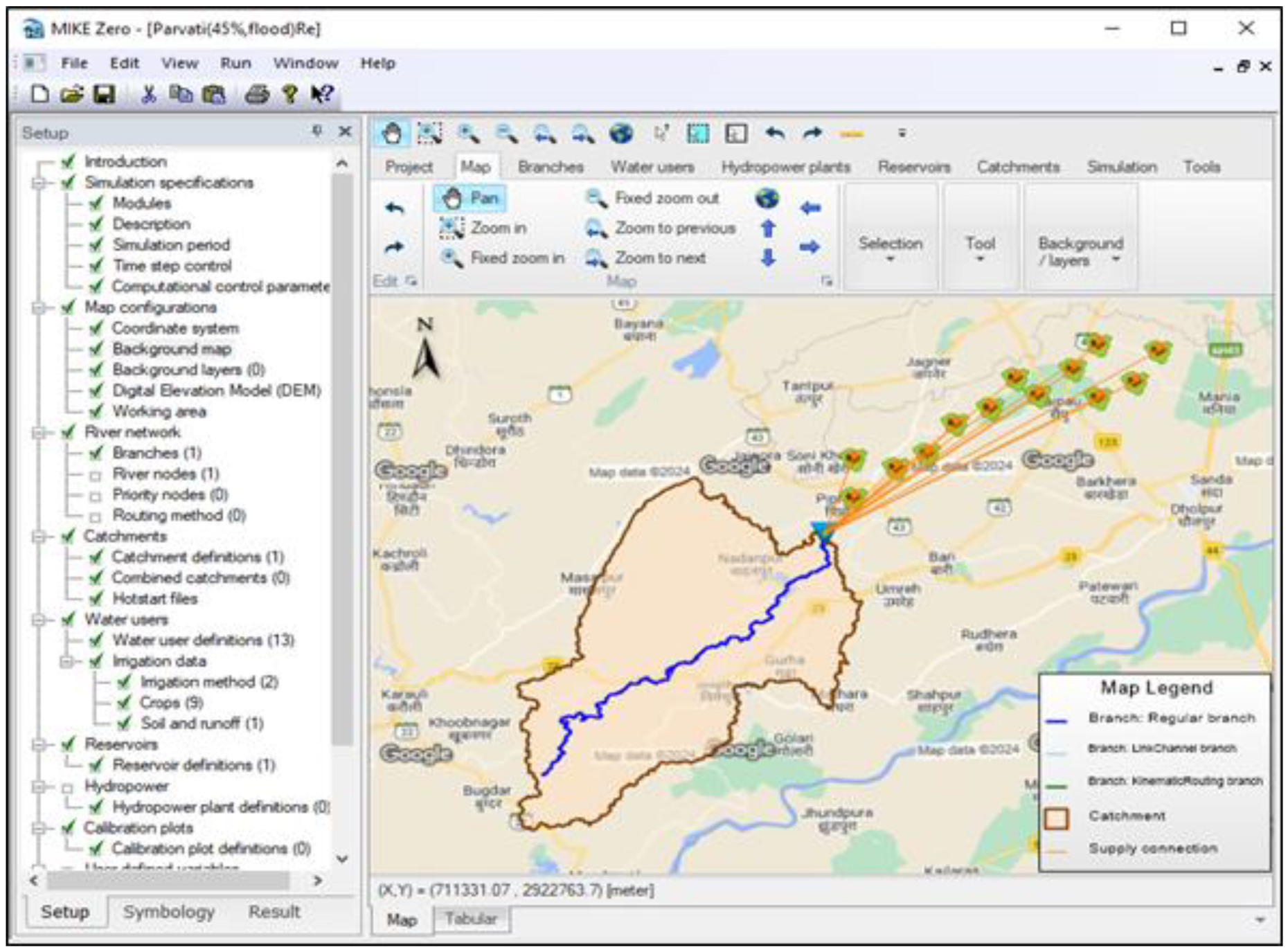
4.3. Calibration of MIKE HYDRO Basin Model
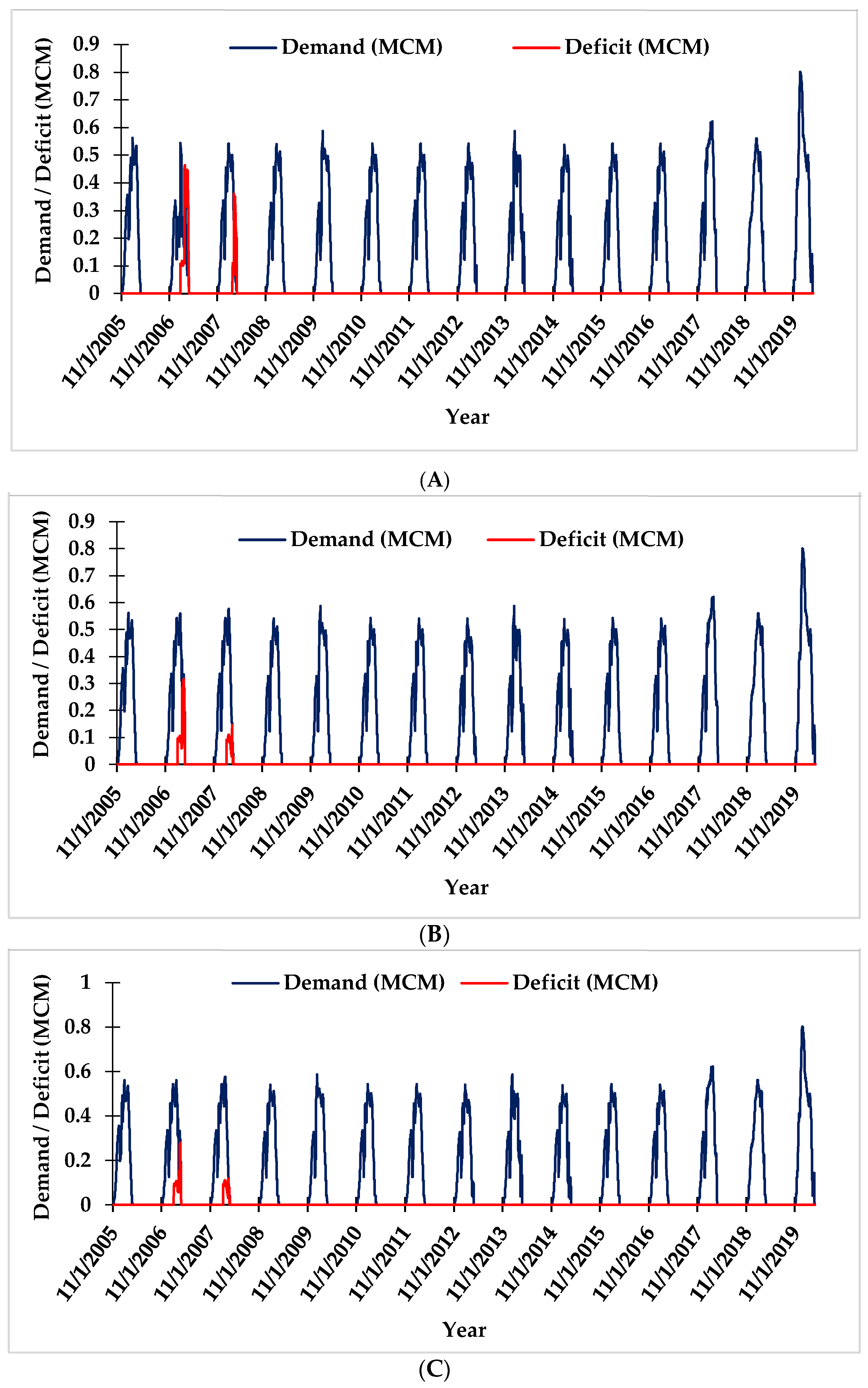
4.4. Water Demand and Deficit Simulation
4.5. Development of Management Scenarios
4.6. Water Demand and Deficit Analysis under Management Scenarios
4.7. Performance Evaluation of Parvati Reservoir System
5. Conclusions
Author Contributions
Funding
Data Availability Statement
Acknowledgments
Conflicts of Interest
References
- Baig, M.A.A.; Mallikarjuna, P.; Krishna Reddy, T.V. Rainfall—Runoff modelling—A case study. ISH J. Hydraul. Eng. 2008, 14, 18–35. [Google Scholar] [CrossRef]
- Yatheendradas, S.; Wagener, T.; Gupta, H.; Unkrich, C.; Goodrich, D.; Schaffner, M.; Stewart, A. Understanding uncertainty in distributed flash flood forecasting for semiarid regions. Water Resour. Res. 2008, 1–17. [Google Scholar] [CrossRef]
- Alitane, A.; Essahlaoui, A.; Van Griensven, A.; Yimer, E.A.; Essahlaoui, N.; Mohajane, M.; Chawanda, C.J.; Van Rompaey, A. Towards a Decision-Making Approach of Sustainable Water Resources Management Based on Hydrological Modeling: A Case Study in Central Morocco. Sustainability 2022, 14, 10848. [Google Scholar] [CrossRef]
- Devia, G.K.; Ganasri, B.P.; Dwarakish, G.S. A Review on Hydrological Models. Aquat. Procedia 2015, 4, 1001–1007. [Google Scholar] [CrossRef]
- Mensah, J.K.; Ofosu, E.A.; Yidana, S.M.; Akpoti, K.; Kabo-bah, A.T. Integrated modeling of hydrological processes and groundwater recharge based on land use land cover, and climate changes: A systematic review. Environ. Adv. 2022, 8, 100224. [Google Scholar] [CrossRef]
- Singh, A.; Malik, A.; Kumar, A.; Kisi, O. Rainfall-runoff modeling in hilly watershed using heuristic approaches with gamma test. Arab. J. Geosci. 2018, 11, 261. [Google Scholar] [CrossRef]
- Ward, P.J.; de Ruiter, M.C.; Mård, J.; Schröter, K.; Van Loon, A.; Veldkamp, T.; von Uexkull, N.; Wanders, N.; AghaKouchak, A.; Arnbjerg-Nielsen, K.; et al. The need to integrate flood and drought disaster risk reduction strategies. Water Secur. 2020, 11, 100070. [Google Scholar] [CrossRef]
- Zhang, X.; Liu, P.; Cheng, L.; Xie, K.; Han, D.; Zhou, L. The temporal variations in runoff-generation parameters of the Xinanjiang model due to human activities: A case study in the upper Yangtze River Basin, China. J. Hydrol. Reg. Stud. 2021, 37, 100910. [Google Scholar] [CrossRef]
- Jothiprakash, V.; Magar, R. Soft computing tools in rainfall-runoff modeling. ISH J. Hydraul. Eng. 2009, 15, 84–96. [Google Scholar] [CrossRef]
- Sahu, R.K.; Mishra, S.K.; Eldho, T.I. Performance evaluation of modified versions of scs curve number method for two watersheds of maharashtra, India. ISH J. Hydraul. Eng. 2012, 18, 27–36. [Google Scholar] [CrossRef]
- Abdulla, F.A.; Lettenmaier, D.P. Development of regional parameter estimation equations for a macroscale hydrologic model. J. Hydrol. 1997, 197, 230–257. [Google Scholar] [CrossRef]
- Venkatesh, B.; Chandramohan, T.; Purandara, B.K.; Jose, M.K.; Nayak, P.C. Modeling of a River Basin Using SWAT Model. In Hydrologic Modeling: Select Proceedings of ICWEES-2016; Springer: Singapore, 2018; pp. 707–714. [Google Scholar] [CrossRef]
- McMichael, C.E.; Hope, A.S.; Loaiciga, H.A. Distributed hydrological modelling in California semi-arid shrublands: MIKE SHE model calibration and uncertainty estimation. J. Hydrol. 2006, 317, 307–324. [Google Scholar] [CrossRef]
- Beven, K.; Bathurst, J.; O’connell, E.N.D.A.; Littlewood, I.; Blackie, J.; Robinson, M. Hydrological modelling. Prog. Mod. Hydrol. Past Present Future 2015, 216–239. [Google Scholar] [CrossRef]
- Boughton, W. The Australian water balance model. Environ. Model. Softw. 2004, 19, 943–956. [Google Scholar] [CrossRef]
- Chiew, F.H.S.; McMahon, T.A. Modelling the impacts of climate change on Australian streamflow. Hydrol. Process. 2002, 16, 1235–1245. [Google Scholar] [CrossRef]
- Gautam, V.K.; Awasthi, M.K. Evaluation of water resources demand and supply for the districts of central Narmada valley zone. Int. J. Curr. Microbiol. App. Sci. 2020, 9, 3043–3050. [Google Scholar] [CrossRef]
- Gautam, V.K.; Awasthi, M.K.; Trivedi, A. Optimum allocation of water and land resource for maximizing farm income of Jabalpur District, Madhya Pradesh. Int. J. Environ. Clim. Change 2020, 10, 224–232. [Google Scholar] [CrossRef]
- Gautam, V.K.; Trivedi, A. Optimal Water Resources Allocation and Crop Planning for Mandla District of Madhya Pradesh. Indian J. Soil Conserv. 2023, 51, 68–75. [Google Scholar]
- Zegait, R.; Bouznad, I.E.; Remini, B.; Bengusmia, D.; Ajia, F.; Guastaldi, E.; Lopane, N.; Petrone, D. Comprehensive model for sustainable water resource management in Southern Algeria: Integrating remote sensing and WEAP model. Model. Earth Syst. Environ. 2024, 10, 1027–1042. [Google Scholar] [CrossRef]
- Jaiswal, R.K.; Ghosh, N.C.; Guru, P.; Devakant. MIKE BASIN Based Decision Support Tool for Water Sharing and Irrigation Management in Rangawan Command of India. Adv. Agric. 2014, 2014, 924948. [Google Scholar] [CrossRef]
- Jaiswal, R.K.; Lohani, A.K.; Tiwari, H.L. A decision support system framework for strategic water resources planning and management under projected climate scenarios for a reservoir complex. J. Hydrol. 2021, 603, 127051. [Google Scholar] [CrossRef]
- Kumar, R.; Huda, M.B.; Maryam, M.; Lone, M.A. Rainfall runoff modeling using MIKE 11 NAM of the Jhelum river in Kashmir Valley, India. Mausam 2022, 73, 365–372. [Google Scholar] [CrossRef]
- Gabor, E.; Beilicci, E.; Beilicci, R. Advanced Hydroinformatic Tools for Modelling of Reservoirs Operation. IOP Conf. Ser. Mater. Sci. Eng. 2019, 471, 42002. [Google Scholar] [CrossRef]
- Pareta, K. Hydrological modelling of largest braided river of India using MIKE Hydro River software with rainfall runoff, hydrodynamic and snowmelt modules. J. Water Clim. Change 2023, 14, 1314–1338. [Google Scholar] [CrossRef]
- Santos, R.M.B.; Fernandes, L.F.S.; Cortes, R.M.V.; Pacheco, F.A.L. Development of a hydrologic and water allocation model to assess water availability in the Sabor river basin (Portugal). Int. J. Environ. Res. Public Health 2019, 16, 2419. [Google Scholar] [CrossRef]
- Yu, Y.; Disse, M.; Yu, R.; Yu, G.; Sun, L.; Huttner, P.; Rumbaur, C. Large-scale hydrological modeling and decision-making for agricultural water consumption and allocation in the main stem Tarim River, China. Water 2015, 7, 2821–2839. [Google Scholar] [CrossRef]
- Moharir, K.N.; Pande, C.B.; Gautam, V.K.; Singh, S.K.; Rane, N.L. Integration of hydrogeological data, GIS and AHP techniques applied to delineate groundwater potential zones in sandstone, limestone and shales rocks of the Damoh district,(MP) central India. Environ. Res. 2023, 228, 115832. [Google Scholar] [CrossRef]
- Gautam, V.K.; Pande, C.B.; Kothari, M.; Singh, P.K.; Agrawal, A. Exploration of groundwater potential zones mapping for hard rock region in the Jakham river basin using geospatial techniques and aquifer parameters. Adv. Space Res. 2023, 71, 2892–2908. [Google Scholar] [CrossRef]
- Allen, R.G.; Smith, M.; Pereira, L.S.; Raes, D.; Wright, J.L. Revised FAO procedures for calculating evapotranspiration: Irrigation and drainage paper no. 56 with testing in Idaho. In Proceedings of the Watershed Management and Operations Management 2000, Fort Collins, CO, USA, 20 June 2000; pp. 1–10. [Google Scholar]
- Jaiswal, R.K.; Kumari, C.; Galkate, R.V.; Lohani, A.K. Assessment of Productivity Based Efficiencies for Optimal Utilization of Water Resources in a Command. Sustain. Water Resour. 2022, 116, 262–282. [Google Scholar] [CrossRef]
- Kumar, A.; Mishra, A.R.; Denis, D.M.; Jeet, P.; Singh, U. Calibration and validation of FAO: Aqua crop model for wheat in Vindhyan region. J. Pharmacogn. Phytochem. 2020, 9, 299–305. [Google Scholar]
- Galkate, R.V.; Jaiswal, R.K.; Thomas, T.; Nayak, T.R. Rainfall runoff modelling using conceptual NAM model. In Proceedings of the International Conference on Sustainability and Management Strategy (ICSMS-2014), Nagpur, India, 21–22 March 2014; Institute of Management and Technology: Nagpur, India, 2014. [Google Scholar]
- Asuero, A.G.; Sayago, A.; González, A.G. The correlation coefficient: An overview. Crit. Rev. Anal. Chem. 2007, 36, 41–59. [Google Scholar] [CrossRef]
- Moriasi, D.N.; Arnold, J.G.; Liew, M.W.; Van Bingner, R.L.; Harmel, R.D.; Veith, T.L. Model evaluation guidelines for systematic quantification of accuracy in watershed simulations. Trans. ASABE 2007, 50, 885–900. [Google Scholar] [CrossRef]
- Willmott, C.J. Some comments on the evaluation of model performance. Bull. Am. Meteorol. Soc. 1982, 63, 1309–1313. [Google Scholar] [CrossRef]
- Gupta, H.V.; Sorooshian, S.; Yapo, P.O. Status of automatic calibration for hydrologic models: Comparison with multilevel expert calibration. J. Hydrol. Eng. 1999, 4, 135–143. [Google Scholar] [CrossRef]
- Knoben, W.J.; Freer, J.E.; Woods, R.A. Inherent benchmark or not? Comparing Nash–Sutcliffe and Kling–Gupta efficiency scores. Hydrol. Earth Syst. Sci. 2019, 23, 4323–4331. [Google Scholar] [CrossRef]
- Sandoval-Solis, S.; McKinney, D.C.; Loucks, D.P. Sustainability index for water resources planning and management. J. Water Resour. Plan. Manag. 2011, 137, 381–390. [Google Scholar] [CrossRef]
- Hashimoto, T.; Stedinger, J.R.; Loucks, D.P. Reliability, Resiliency, and Vulnerability Criteria For Water Resource System Performance Evaluation. Water Resour. Res. 1982, 18, 14–20. [Google Scholar] [CrossRef]
- Kjeldsen, T.R.; Rosbjerg, D. Choice of reliability, resilience and vulnerability estimators for risk assessments of water resources systems/Choix d’estimateurs de fiabilité, de résilience et de vulnérabilité pour les analyses de risque de systèmes de ressources en eau. Hydrol. Sci. J. 2004, 49, 767. [Google Scholar] [CrossRef]
- Kahsay, K.D.; Pingale, S.M.; Hatiye, S.D. Impact of climate change on groundwater recharge and base flow in the sub-catchment of Tekeze basin, Ethiopia. Groundw. Sustain. Dev. 2018, 6, 121–133. [Google Scholar] [CrossRef]
- Vansteenkiste, T.; Tavakoli, M.; Van Steenbergen, N.; De Smedt, F.; Batelaan, O.; Pereira, F.; Willems, P. Intercomparison of five lumped and distributed models for catchment runoff and extreme flow simulation. J. Hydrol. 2014, 511, 335–349. [Google Scholar] [CrossRef]
- Odiyo, J.O.; Phangisa, J.I.; Makungo, R. Rainfall-runoff modelling for estimating Latonyanda River flow contributions to Luvuvhu River downstream of Albasini Dam. Phys. Chem. Earth 2012, 50–52, 5–13. [Google Scholar] [CrossRef]
- Filianoti, P.; Gurnari, L.; Zema, D.A.; Bombino, G.; Sinagra, M.; Tucciarelli, T. An evaluation matrix to compare computer hydrological models for flood predictions. Hydrology 2020, 7, 42. [Google Scholar] [CrossRef]
- Aredo, M.R.; Hatiye, S.D.; Pingale, S.M. Modeling the rainfall-runoff using MIKE 11 NAM model in Shaya catchment, Ethiopia. Model. Earth Syst. Environ. 2021, 7, 2545–2551. [Google Scholar] [CrossRef]
- DHI. MIKE 11-A Modelling System for Rivers and Channels: User Guide; Danish Hydraulic Institute: Horsholm, Denmark, 2017. [Google Scholar]
- Alotaibi, M.; Alhajeri, N.S.; Al-Fadhli, F.M.; Al Jabri, S.; Gabr, M. Impact of Climate Change on Crop Irrigation Requirements in Arid Regions. Water Resour. Manag. 2023, 37, 1965–1984. [Google Scholar] [CrossRef]
- Hatfield, J.L.; Dold, C. Water-use efficiency: Advances and challenges in a changing climate. Front. Plant Sci. 2019, 10, 103. [Google Scholar] [CrossRef] [PubMed]
- Iglesias, A.; Garrote, L. Adaptation strategies for agricultural water management under climate change in Europe. Agric. Water Manag. 2015, 155, 113–124. [Google Scholar] [CrossRef]
- Srivastav, A.L.; Dhyani, R.; Ranjan, M.; Madhav, S.; Sillanpää, M. Climate-resilient strategies for sustainable management of water resources and agriculture. Environ. Sci. Pollut. Res. 2021, 28, 41576–41595. [Google Scholar] [CrossRef]
- Fereres, E.; Soriano, M.A. Deficit irrigation for reducing agricultural water use. J. Exp. Bot. 2007, 58, 147–159. [Google Scholar] [CrossRef]
- Du, T.; Kang, S.; Zhang, J.; Davies, W.J. Deficit irrigation and sustainable water-resource strategies in agriculture for China’s food security. J. Exp. Bot. 2015, 66, 2253–2269. [Google Scholar] [CrossRef]
- Allen, L.N.; MacAdam, J.W. Irrigation and water management. Forages Sci. Grassl. Agric. 2020, 2, 497–513. [Google Scholar]
- Kumar, J.; Biswas, B.; Walker, S. Multi-temporal LULC classification using hybrid approach and monitoring built-up growth with Shannon’s entropy for a semi-arid region of Rajasthan, India. J. Geol. Soc. India 2020, 95, 626–635. [Google Scholar] [CrossRef]
- Mazahir, S.; Javed, A.; Khanday, M.Y. Assessing Spatio-Temporal Land Cover Changes in Dhund River Basin, Eastern Rajasthan (India), Using Multi-Temporal Landsat Data. J. Geogr. Inf. Syst. 2024, 16, 244–258. [Google Scholar] [CrossRef]
- Meraj, M.; Javed, A. Land Use/Land Cover (LULC) Dynamics in a Semi-Arid Watershed in Eastern Rajasthan, India Using Geospatial Tools. J. Geogr. Inf. Syst. 2022, 14, 612–633. [Google Scholar] [CrossRef]
- Hazbavi, Z.; Baartman, J.E.; Nunes, J.P.; Keesstra, S.D.; Sadeghi, S.H. Changeability of reliability, resilience and vulnerability indicators with respect to drought patterns. Ecol. Indic. 2018, 87, 196–208. [Google Scholar] [CrossRef]
- Malek, K.; Adam, J.C.; Stöckle, C.O.; Peters, R.T. Climate change reduces water availability for agriculture by decreasing non-evaporative irrigation losses. J. Hydrol. 2018, 561, 444–460. [Google Scholar] [CrossRef]
- Wada, Y.; van Beek, L.P.; Bierkens, M.F. Modelling global water stress of the recent past: On the relative importance of trends in water demand and climate variability. Hydrol. Earth Syst. Sci. 2011, 15, 3785–3808. [Google Scholar] [CrossRef]
- Yin, L.; Wang, L.; Keim, B.D.; Konsoer, K.; Zheng, W. Wavelet Analysis of Dam Injection and Discharge in Three Gorges Dam and Reservoir with Precipitation and River Discharge. Water 2022, 14, 567. [Google Scholar] [CrossRef]
- Zhou, G.; Tang, Y.; Zhang, W.; Liu, W.; Jiang, Y.; Gao, E.; Bai, Y. Shadow Detection on High-Resolution Digital Orthophoto Map Using Semantic Matching. IEEE Trans. Geosci. Remote Sens. 2023, 61, 1–20. [Google Scholar] [CrossRef]
- Li, J.; Pang, Z.; Liu, Y.; Hu, S.; Jiang, W.; Tian, L.; Tian, J. Changes in groundwater dynamics and geochemical evolution induced by drainage reorganization: Evidence from 81Kr and 36Cl dating of geothermal water in the Weihe Basin of China. Earth Planet. Sci. Lett. 2023, 623, 118425. [Google Scholar] [CrossRef]
- Dai, Z.; Peng, L.; Qin, S. Experimental and numerical investigation on the mechanism of ground collapse induced by underground drainage pipe leakage. Environ. Earth Sci. 2023, 83, 32. [Google Scholar] [CrossRef]
- Dai, Z.; Ritzi, R.W., Jr.; Dominic, D.F. Improving permeability semivariograms with transition probability models of hierarchical sedimentary architecture derived from outcrop analog studies. Water Resour. Res. 2005, 41, 1–13. [Google Scholar] [CrossRef]
- Dai, Z.; Samper, J. Inverse problem of multicomponent reactive chemical transport in porous media: Formulation and applications. Water Resour. Res. 2004, 40, 1–18. [Google Scholar] [CrossRef]
- Liu, C.; Shan, Y.; He, L.; Li, F.; Liu, X.; Nepf, H. Plant Morphology Impacts Bedload Sediment Transport. Geophys. Res. Lett. 2024, 51, e2024GL108800. [Google Scholar] [CrossRef]
- Li, Z.; He, M.; Li, B.; Wen, X.; Zhou, J.; Cheng, Y.; Deng, L. Multi-isotopic composition (Li and B isotopes) and hydrochemistry characterization of the Lakko Co Li-rich salt lake in Tibet, China: Origin and hydrological processes. J. Hydrol. 2024, 630, 130714. [Google Scholar] [CrossRef]
- Yin, L.; Wang, L.; Li, T.; Lu, S.; Yin, Z.; Liu, X.; Zheng, W. U-Net-STN: A Novel End-to-End Lake Boundary Prediction Model. Land 2023, 12, 1602. [Google Scholar] [CrossRef]
- Yin, L.; Wang, L.; Keim, B.D.; Konsoer, K.; Yin, Z.; Liu, M.; Zheng, W. Spatial and wavelet analysis of precipitation and river discharge during operation of the Three Gorges Dam, China. Ecol. Indic. 2023, 154, 110837. [Google Scholar] [CrossRef]
- Yin, L.; Wang, L.; Li, T.; Lu, S.; Tian, J.; Yin, Z.; Zheng, W. U-Net-LSTM: Time Series-Enhanced Lake Boundary Prediction Model. Land 2023, 12, 1859. [Google Scholar] [CrossRef]
- Zhou, G.; Lin, G.; Liu, Z.; Zhou, X.; Li, W.; Li, X.; Deng, R. An optical system for suppression of laser echo energy from the water surface on single-band bathymetric LiDAR. Opt. Lasers Eng. 2023, 163, 107468. [Google Scholar] [CrossRef]
- Zhou, G.; Xu, C.; Zhang, H.; Zhou, X.; Zhao, D.; Wu, G.; Zhang, L. PMT gain self-adjustment system for high-accuracy echo signal detection. Int. J. Remote Sens. 2022, 43, 7213–7235. [Google Scholar] [CrossRef]
- Zhang, K.; Li, Y.; Yu, Z.; Yang, T.; Xu, J.; Chao, L.; Lin, Z. Xin’anjiang Nested Experimental Watershed (XAJ-NEW) for Understanding Multiscale Water Cycle: Scientific Objectives and Experimental Design. Engineering 2022, 18, 207–217. [Google Scholar] [CrossRef]
- Hu, C.; Dong, B.; Shao, H.; Zhang, J.; Wang, Y. Toward Purifying Defect Feature for Multilabel Sewer Defect Classification. IEEE Trans. Instrum. Meas. 2023, 72, 5008611. [Google Scholar] [CrossRef]
- Ye, X.; Zhu, H.; Chang, F.; Xie, T.; Tian, F.; Zhang, W.; Catani, F. Revisiting spatiotemporal evolution process and mechanism of a giant reservoir landslide during weather extremes. Eng. Geol. 2024, 332, 107480. [Google Scholar] [CrossRef]
- Di, D.; Li, T.; Fang, H.; Xiao, L.; Du, X.; Sun, B.; Li, B. A CFD-DEM investigation into hydraulic transport and retardation response characteristics of drainage pipeline siltation using intelligent model. Tunn. Undergr. Space Technol. 2024, 152, 105964. [Google Scholar] [CrossRef]


| Statistical Indices | Formula | Range | Performance Rating |
|---|---|---|---|
| Nash–Sutcliff Efficiency (NSE) | 0.75 < NSE ≤ 1.00 | Very good | |
| 0.65 < NSE ≤ 0.75 | Good | ||
| 0.50 < NSE ≤ 0.65 | Satisfactory | ||
| NSE ≤ 0.50 | Unsatisfactory | ||
| Coefficient of Determination (R2) | R2 ≥ 0.8 | Very good | |
| 0.6 ≤ R2 ≤ 0.8 | Good | ||
| 0.4 ≤ R2 ≤ 0.6 | Satisfactory | ||
| R2 ≤0.4 | Unsatisfactory | ||
| Root Mean Square Error (RMSE) | Less than half of the standard deviation of the observed dataset | Good | |
| Percentage of Bias (PBIAS) | PBIAS < ±10 | Very good | |
| ±10 ≤ PBIAS ≤ ±15 | Good | ||
| ±15 ≤ PBIAS ≤ ±25 | Satisfactory | ||
| PBIAS ≥ ±25 | Unsatisfactory | ||
| RMSE-observations standard deviation ratio | 0 ≤ RSR ≤ 0.50 | Very good | |
| 0.50 ≤ RSR ≤ 0.60 | Good | ||
| 0.60 ≤ RSR ≤ 0.70 | Satisfactory | ||
| RSR > 0.70 | Unsatisfactory | ||
| Kling–Gupta Efficiency (KGE) | 0.8 ≤ KGE ≤ 1 | Very good | |
| 0.6 ≤ KGE ≤ 0.8 | Good | ||
| 0.4 ≤ KGE ≤ 0.6 | Satisfactory | ||
| 0.4 < KGE | Unsatisfactory |
| Parameter | Unit | Common Range | Best Fit Value |
|---|---|---|---|
| Umax | mm | 5–20 | 5.16 |
| Lmax | mm | 100–300 | 250 |
| CQOF | - | 0.1–1 | 0.20 |
| CKIF | mm | 100–1000 | 664.2 |
| TOF | - | 0–0.99 | 0.70 |
| TIF | - | 0–0.99 | 0.3 |
| TG | - | 0–0.99 | 0.479 |
| CK12 | hrs | 3–72 | 56.5 |
| CKBF | hrs | 1000–4000 | 3259 |
| Conveyance Efficiency (ηc) | Irrigation Method | GW Use | Scenario No. | Demand (MCM) | Deficit (MCM) | Rel | Vul | Res | SI |
|---|---|---|---|---|---|---|---|---|---|
| 45% | Flood | 0% | BP-0 | 42.795 | 3.451 | 0.533 | 0.467 | 0.457 | 0.506 |
| 45% | Flood | 5% | BP-1 | 42.795 | 1.819 | 0.835 | 0.165 | 0.603 | 0.749 |
| 65% | Flood | 0% | BP-2 | 42.795 | 0.753 | 0.812 | 0.188 | 0.471 | 0.677 |
| 65% | Flood | 5% | BP-3 | 42.795 | 0.644 | 0.877 | 0.123 | 0.714 | 0.819 |
| 75% | Flood | 0% | BP-4 | 42.795 | 0.214 | 0.895 | 0.105 | 0.658 | 0.807 |
| 75% | Flood | 5% | BP-5 | 42.795 | 0.052 | 0.957 | 0.043 | 0.857 | 0.922 |
| 95% | Sprinkler | 0% | BP-6 | 42.795 | 0.00 | 1.000 | 0.000 | 1.000 | 1.000 |
Disclaimer/Publisher’s Note: The statements, opinions and data contained in all publications are solely those of the individual author(s) and contributor(s) and not of MDPI and/or the editor(s). MDPI and/or the editor(s) disclaim responsibility for any injury to people or property resulting from any ideas, methods, instructions or products referred to in the content. |
© 2024 by the authors. Licensee MDPI, Basel, Switzerland. This article is an open access article distributed under the terms and conditions of the Creative Commons Attribution (CC BY) license (https://creativecommons.org/licenses/by/4.0/).
Share and Cite
Agrawal, A.; Kothari, M.; Jaiswal, R.K.; Gautam, V.K.; Pande, C.B.; Ahmed, K.O.; Refadah, S.S.; Khan, M.Y.A.; Abdulqadim, T.J.; Đurin, B. Integrated Basin-Scale Modelling for Sustainable Water Management Using MIKE HYDRO Basin Model: A Case Study of Parvati Basin, India. Water 2024, 16, 2739. https://doi.org/10.3390/w16192739
Agrawal A, Kothari M, Jaiswal RK, Gautam VK, Pande CB, Ahmed KO, Refadah SS, Khan MYA, Abdulqadim TJ, Đurin B. Integrated Basin-Scale Modelling for Sustainable Water Management Using MIKE HYDRO Basin Model: A Case Study of Parvati Basin, India. Water. 2024; 16(19):2739. https://doi.org/10.3390/w16192739
Chicago/Turabian StyleAgrawal, Abhishek, Mahesh Kothari, R. K. Jaiswal, Vinay Kumar Gautam, Chaitanya Baliram Pande, Kaywan Othman Ahmed, Samyah Salem Refadah, Mohd Yawar Ali Khan, Tuhami Jamil Abdulqadim, and Bojan Đurin. 2024. "Integrated Basin-Scale Modelling for Sustainable Water Management Using MIKE HYDRO Basin Model: A Case Study of Parvati Basin, India" Water 16, no. 19: 2739. https://doi.org/10.3390/w16192739
APA StyleAgrawal, A., Kothari, M., Jaiswal, R. K., Gautam, V. K., Pande, C. B., Ahmed, K. O., Refadah, S. S., Khan, M. Y. A., Abdulqadim, T. J., & Đurin, B. (2024). Integrated Basin-Scale Modelling for Sustainable Water Management Using MIKE HYDRO Basin Model: A Case Study of Parvati Basin, India. Water, 16(19), 2739. https://doi.org/10.3390/w16192739