Abstract
With the recent acceleration in urbanisation and industrialisation, industrial pollution has severely impacted inland water bodies and ecosystem services globally, causing significant restrains to freshwater availability and myriad damages to benthic species. The Kelani River Basin in Sri Lanka, covering only ~3.6% of the land but hosting over a quarter of its population and many industrial zones, is identified as the most polluted watershed in the country. This study used unsupervised learning (UL) and an indexing approach to identify potential industrial pollutant sources along the Kelani River. The UL results were compared with those obtained from a novel Industrial Pollution Index (IPI). Three latent variables related to industrial pollution were identified via Factor Analysis of monthly water quality data from 17 monitoring stations from 2016 to 2020. The developed IPI was validated using a Long Short-Term Memory Artificial Neural Network model (NSE = 0.98, RMSE = 0.81), identifying Cd, Zn, and Fe as the primary parameters influencing river pollution status. The UL method identified five stations with elevated concentrations for the developed latent variables, and the IPI confirmed four of them. Based on the findings from both methods, the industrial zones along the Kelani River have emerged as a likely source of pollution in the river’s water. The results suggest that the proposed method effectively identifies industrial pollution sources, offering a scalable methodology for other river basins to ensure sustainable water resource management.
1. Introduction
Water pollution is an escalating global issue aggravated by climate change, industrialisation, and urbanisation [1]. Among many other related factors, the rapid acceleration of global industrialisation stands out for its significant consequences on surface and sub-surface water bodies, including rivers, lakes, and groundwater reserves. Therefore, water pollution from industrial wastewater is a critical concern, impacting human health, causing habitat destruction, and leading to ecosystem degradation [2]. Approximately 80% of industrial and domestic wastewater worldwide is discharged into water resources without undergoing any form of pre-treatment [3]. Consequently, these untreated effluents significantly threaten human well-being, aquatic life diversity, and water resources quality.
Globally, the water quality of rivers, lakes, and groundwater remains uncertain for over 3 billion people due to insufficient assessment and a lack of data, placing them at risk of diseases [4]. The consequences of such lapses in water quality assessments are exacerbated by industrial pollution. Primarily being a point source issue with identifiable origins, such as factories and processing plants [5], industrial pollution exerts far-reaching impacts on water bodies, affecting numerous water quality parameters, including organic matter, heavy metals like cadmium, iron, lead, and zinc, and nutrients such as nitrate and sulphate [6,7]. Heavy metals can accumulate in aquatic organisms, posing significant threats to food safety and human health, while excessive nitrate can cause eutrophication, leading to harmful algal blooms and oxygen depletion in rivers. These conditions impair water quality for drinking and recreational purposes and increase the health risks for living organisms [8,9]. The rapid urbanisation driven by industrialisation intensifies the demand for safe and clean water, making the control of industrial pollution in freshwater bodies critically important.
Although pollution due to industrial effluents is a global concern, only a few studies have been conducted to identify the sources of industrial pollution in source catchments. Machine learning efficiently identifies pollution sources, predicts trends, and uncovers complex relationships between variables in source catchments [10,11]. Techniques include supervised learning (e.g., regression and classification), unsupervised learning (e.g., pattern identification), and reinforcement learning [12]. Buras et al. [13] suggested a random forest and gradient-boosting machine learning approach to identify industrial pollutant types in wastewater bodies and to determine the point of origin. Xia et al. [14] proposed a methodology to quantify heavy metal pollution sources using multivariate statistical techniques and Geographical Information System (GIS) technology in an urban river system. Wang et al. [15] proposed an approach to identify the sources of heavy metal pollution and the spatial distribution of the contaminants by combining Principal Component Analysis (PCA) and Cluster Analysis (CA). According to Barati et al. [16], few stochastic methods for identifying pollutant sources have been proposed while highlighting the importance of methods that can be applied in large and complex catchments without prior knowledge of pollutant sources.
The indexing approach is a valuable tool for tracking and identifying a specific type of pollution in water bodies. For example, the Water Pollution Index (WPI) describes the pollution status of a waterbody by summarising complex water quality information into one singular numerical value [17,18]. Several studies have used these indices to assess heavy metal contamination levels in rivers and lakes [19,20,21,22]. Although heavy metal pollution indexes serve as a valuable tool for evaluating pollution status in water bodies, existing indices do not adequately account for the variability in industrial pollutants in diverse catchments. In addition to identifying pollutant sources using the indexing approach, several studies have used multivariate statistical techniques, such as PCA [23,24], Factor Analysis (FA) [25,26], and Cluster Analysis (CA) [27,28,29] to identify the spatial and seasonal variations in water quality. These methods have become even more productive since the evolution of artificial intelligence and machine learning [30,31], allowing for the use of (more flexible) approaches, such as unsupervised learning techniques, to find hidden/unknown patterns in complex datasets using dimensionality reduction (e.g., PCA and FA) and pattern recognition (e.g., CA) techniques [32,33].
Industrial pollutants in a specific river can vary based on the types of industries, land use, and geogenic processes in the catchment [34]. The related literature lacks scalable methods for evaluating specific types of pollution in river systems while considering the unique pollutant contribution. Therefore, this study aims to develop and validate an independent, dual-method framework that uses unsupervised machine learning techniques and a novel Industrial Pollution Index (IPI) to identify and quantify industrial pollution sources in river basins. Focusing on the Kelani River Basin in Sri Lanka, this study seeks to assess pollution patterns through separate analyses and provide a robust methodology for pollution source identification, which can be adapted for other catchment areas. The Kelani River Basin covers only ~3.6% of the country’s land area but hosts over a quarter of its population and many industrial zones. It is also identified as the most polluted watershed in the country [35]. Rather than combining the methods, this approach independently evaluates pollution status using factor and cluster analyses and then compares the results to triangulate key industrial pollution sources. The validation of the IPI through advanced machine learning models (Random Forest and LSTM ANN) ensures the highly accurate detection of pollution severity and distribution. This independent yet comparative approach offers a scalable and adaptable framework for water pollution assessments in other river basins, distinguishing it from prior methodologies that integrate or combine techniques.
2. Materials and Methods
2.1. Study Area
The Kelani River Basin (KRB), covering an area of 2230 km2 in western Sri Lanka, nourishes the country’s fourth longest river, the Kelani River. It originates from the central highlands and flows through the capital city, Colombo, before emptying into the Indian Ocean [36] (Figure 1). The river catchment receives an annual rainfall of ~3720 mm, distributed across four distinct seasons: (1) The Southwest Monsoon (SWM; May–September), (2) Inter-monsoon 1 (IM1, October–November), (3) Northeast Monsoon (NEM, December–February), and (4) Inter-monsoon 2 (IM2, March–April), in which the SWM (53%) and NEM (9%) contribute the most and the least of the yearly precipitation. Multiple drinking water intakes along the Kelani River supply treated water to the Greater Colombo area, accounting for about 80% of the region’s water supply for a population of ~640,000 [37,38].
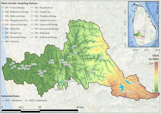
Figure 1.
Kelani River Basin and the water quality sampling stations within the study area. The topography of the basin (m MSL) was derived from Digital Elevation Model (DEM) data from the Shuttle Radar Topography Mission (SRTM: https://www.earthdata.nasa.gov/sensors/srtm, accessed on 24 May 2024).
According to the records, by 2020, 2842 industries were located inside the KRB [39]. The Central Environmental Authority (CEA) has categorised these industries into three groups (Type A, B, and C) by considering the attributable environmental impacts, where Type A includes significantly high-polluting industrial activities. About 30% of the industries located in the KRB are Type A, while Type B and C, respectively, account for 43% and 27% of the industries in the region [39,40]. Two export-processing industrial zones (viz., Biyagama and Seethawake Industrial Zones) with diverse industrial facilities (e.g., rubber manufacturing, pharmaceuticals, soap/detergent factories, and textile and apparel industries) are also located in the KRB [36,41]. Wastewater discharges from these industrial facilities are regulated by the Environment Protection License (EPL) schemes implemented under the 1980 National Environmental Act [40], which mandates that the wastewater discharged by the industries be treated up to a regulatory value(s) stipulated. Even though the industries must obtain their respective EPLs, no robust monitoring mechanism exists to evaluate effluent discharge qualities and control the pollutant loads discharged into the Kelani River.
2.2. Overall Research Methodology
Figure 2 illustrates the research methodology adopted in this study. First, water quality data were collected from the CEA, and key industrial pollutants were identified based on relevant literature. The study employed two distinct methods to determine industrial pollutant sources. The first method involved Factor Analysis and Cluster Analysis to identify the spatial variation in latent variables across the monitoring stations. The second method applied a water pollution indexing approach, which used rating curves and weighted sub-index values to develop an Industrial Pollution Index (IPI) and conducted an aggregative analysis of the water quality data. Both methods were developed following standard guidelines and literature to ensure accurate identification of pollution sources. The next four sections (Section 2.3, Section 2.4, Section 2.5 and Section 2.6) provide detailed descriptions of each method used in this study.
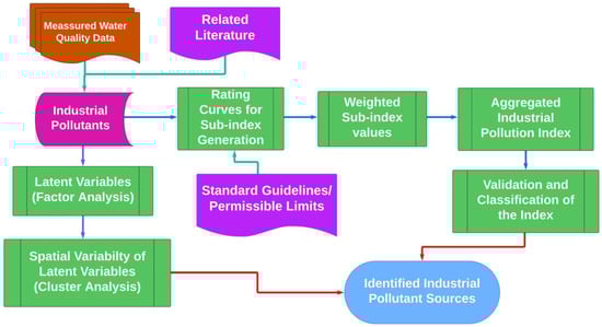
Figure 2.
Descriptive flowchart of the proposed research methodology.
2.3. Data Collection
The Central Environmental Authority of Sri Lanka has established and maintains 17 water quality monitoring stations along the Kelani River (Figure 1). These stations conduct monthly assessments to detect physical, chemical, heavy metal, and microbiological pollutants in the river’s water. Based on the literature [6,7,20,42] and the availability of measured data between 2016 and 2020, six water quality parameters (viz., nitrate, iron (Fe), cadmium (Cd), chromium (Cr), lead (Pb), and zinc (Zn)) were chosen as indicators of industrial pollution considered in this study.
2.4. Machine Learning Approach: Unsupervised Learning
2.4.1. Factor Analysis (FA)
The FA technique has proven helpful in identifying latent patterns and relationships when there is a substantial number of input parameters. This method effectively simplifies the data into a more concise set of elements, explaining most of the variation [25,26]. It is an unsupervised learning technique performed by identifying latent patterns or relationships. In FA, the variable p denotes the quantity of water quality parameters (X1, X2, …, Xp), whereas the variable m denotes the amount of underlying latent variables (LVs) (LV1, LV2, …, LVm). Each water quality parameter, Xj, is expressed as a function of the latent variables. Accordingly, there are m latent variables, and each observed water quality parameter results from a linear combination of these LVs and a residual variate. This FA model aims to develop the highest degrees of correlation accurately. The factor loadings (aj1, aj2, …, ajm) indicate the impact of the latent variable on the water quality parameter. The residual variate is represented by the symbol ej in the following manner (1), where j is the number of latent variables (1, 2, ….., m) [25,26].
The eigenvalues and scree plots determine the optimal number of LVs to retain, and Kaiser’s criterion [43] is one of the methods employed to determine the optimal amount of retained latent variables (LVs), where all LVs with eigenvalues greater than one are preserved. The Kaiser–Meyer–Olkin (KMO) test and Bartlett’s test were used to determine the suitability of a dataset for FA. In FA, the factor loadings are subjected to rotation once the LVs are estimated from the model. This rotation aims to provide a more simplified and easily understandable structure, which helps identify the specific water quality parameters that influence a particular LV. According to Asuero et al. [44], Varimax rotation and Promax rotation are the two most often used methods for rotation. Based on the literature [26,27], this study used the varimax rotation method to rotate LVs.
2.4.2. Self-Organising Map
The Self-Organising Map (SOM) is an unsupervised neural network that clusters data based on group similarities [45]. It utilises an iterative approximation process to transform a collection of vectors from a space with many dimensions to a space with fewer dimensions while preserving the original spatial relationships among the vectors. The technique described is employed to represent and display data nonlinearity. The SOM technique in this study was utilised to examine the spatial variations in the LVs. Compared to a conventional feedforward network, a Self-Organising Map (SOM) is structured in grids of many dimensions. The position of a node in the grid corresponds to a concentrated area in the higher-dimensional state space. The node becomes active when the network receives a vector from its corresponding region in state space. This mapping is probabilistic yet consistent. During the training phase, vectors are randomly dispersed around the grid. This approach ensures that the winning node achieves the highest activation while the activations of nearby nodes are decreased. Ultimately, a single output node is engaged for every collection of vectors. All vectors that prompt the same output node response can be considered in the cluster [46,47].
In this study, the term “vectors” is used to describe the individual data points of the LVs. The “n-dimensional grids” denote the total number of data entries corresponding to the number of water quality measurement stations. The SOM algorithm aims to decrease the dimensionality of the given data to detect and identify the clusters. The study utilised SOM to categorise 17 water quality monitoring sites into distinct clusters based on the variability of LVs.
2.5. Indexing Approach: Industrial Pollution Index (IPI)
The Industrial Pollution Index (IPI), which is a subcategory of the general Water Pollution Index (WPI), is developed in four stages: selection of parameters, sub-indexing of parameters, weighting of parameters, and the aggregation of the sub-index values [48]. The following sub-headings describe each method employed in this study.
2.5.1. Parameter Identification and Sub-Indexing
The literature on industrial pollution was referred to in selecting the parameters for developing the IPI [6,7,42,49]. Accordingly, six water quality parameters measured at 17 locations along the Kelani River (viz., nitrate, Fe, Cd, Cr, Pb, and Zn) were used for developing the Kelani River Basin–Industrial Pollution Index (KRB-IPI).
For a pollution assessment, parameters are selected to represent the specific type of targeted pollution, such as industrial pollution, considered in this study. Sub-index functions are developed to convert the selected parameter concentrations into a unitless value [50]. The sub-index can be developed based on rating curves or interpolation techniques using the water quality standards recommended by the local authorities (Appendix A). The sub-index values convert the parameter concentrations into a dimensionless value. The sub-index value ranges from zero (0) (minimum pollution) to 100 (maximum pollution). In this study, the methods proposed by Hallock [51] and Casillas-García et al. [52] were used to develop rating curves accommodating the local standard limits. The first step was to compare the observations with the particular water quality standard limits (Vperm) to determine the number of observations that exceeded the standards within the analysis period. Subsequently, the dataset was divided into two subsets: observations less than or equal to or those higher than the permissible values. A sub-index value (Qi) was assigned to the permissible limit (Qi,perm) depending on the percentage of the observations that exceeded the standard limit,
where 0 ≤ Pe ≤1 is the proportion of observations that exceeded the standard limit of each parameter.
Qi,perm = 50 + 15Pe
Accordingly, the sub-index took the minimum values of 50 and 65 when all the observations were lower than and exceeded the standard limit, respectively. For the development of rating curves, the quantiles 0, 0.1, 0.8, 0.95, 0.99, and 1 for the subset of observations lower than the standard limit were calculated, and the sub-index (Qi) was assigned using the following equations presented in Table 1.

Table 1.
Sub-index (Qi) values for observations lower and higher than the standard limit for each quantile.
2.5.2. Parameter Weighting
Parameter weighting is performed to find the relative importance and the impact of the selected water quality parameters concerning the river’s pollution status [53]. Most studies have used the Delphi technique to assign the parameter weights [48,53], but more recent studies have started using more data-driven approaches to assign the parameter weights [54,55]. Data-driven approaches tend to use more statistical approaches in determining the weights while considering the water quality standards imposed by the authorities. Initially, the water pollution status was assessed by comparing the measured values with the standard limit using a simple binary function to obtain parameter weight values. If all water quality parameters met the guideline limit, the status was assigned a binary value of 0, indicating ‘unpolluted’. Conversely, if any parameter exceeded the standard limit, a binary value of 1 was assigned, indicating ‘polluted’ [56]. When a parameter’s value exceeded the standard limit, the measured concentration was replaced with the difference between the measured and standard limits. If the parameter value did not exceed the limit, the concentration was replaced with a value of zero (0). This method allows for the incorporation of the frequency and magnitude of standard limit exceedances to determine the river’s initial pollution status. A Random Forest (RF) model was then employed to assess the parameters and identify their relative importance to the initial pollution status. Further, the Rank Order Centroid (ROC) approach was used to assign weights to the parameters, and these weights were validated by comparing them with the relative importance derived from the RF model.
Random Forest (RF) Model
In applying the Random Forest (RF) model to assess water quality, the model constructs an ensemble of decision trees to enhance the accuracy and stability of predictions related to water quality parameters. The RF algorithm introduces two layers of randomisation to improve model robustness. First, it randomly selects samples from the water quality dataset to form the root node samples for each decision tree, ensuring a diverse representation of the data [57]. Additionally, a random subset of potential water quality parameters is chosen at each node of the tree. The model selects the most appropriate parameter from this subset to create a split, driving the decision process. This method of random resampling and parameter selection leads to the creation of multiple decision trees, each contributing to the final model. The collective prediction is obtained by aggregating the outcomes from all trees through majority voting or averaging. This approach allows the RF model to evaluate the relative importance of each water quality parameter, ultimately providing a comprehensive understanding of how these parameters influence the overall water quality assessment. In-depth discussions on the RF model are presented by [58,59].
Rank Order Centroid (ROC) Method
In a water quality study, the Rank Order Centroid (ROC) approach provides a straightforward method for assigning weights to various water quality parameters [60]. In this approach, rankings are produced based on the data distribution of the water quality parameters, and these ranks are then converted into weights. The ROC method minimises the maximum error by identifying the centroid of all possible weight distributions while preserving the rank order derived from the data. The ROC weights (wi) of a set of N variables, ranked from i = 1 to N, are calculated according to the following:
2.5.3. Parameter Aggregation and Classification
Aggregation combines the weighted sub-index value into a single water pollution value, which determines the overall pollution status of the water body [61]. Several weighted and unweighted sub-index aggregation functions are presented in the literature [48,62,63]. The aggregation functions follow either an additive form, a multiplicative form, or a maximum/minimum operator form [49]. The suitable aggregation function for the developed index is selected based on four criteria [64]. The selected aggregation function should minimise the ambiguity problem, which arises when the final index exceeds the critical level without any parameters exceeding the critical level. Secondly, the selected aggregation function should minimise the eclipsing problem, which arises when the aggregated index value is low, although the parameter sub-index values are high. Thirdly, the selected aggregation function should be sensitive to all the changes in individual sub-index values and, finally, the aggregation function should be easy to apply.
Based on the literature, five mostly used aggregation functions were selected for this study. For N number of water quality parameters, ranked from i = 1 to N where the sub-index value of the i-th parameter is Si, and the weight of the i-th parameter is Wi:
Subsequently, a sensitivity analysis was conducted to determine the most appropriate aggregation function for the developed KRB-IPI. The aggregation function that exhibited the highest sensitivity to changes in parameter values was selected as the optimal choice for the pollution index. A Long Short-Term Memory (LSTM) Artificial Neural Network (ANN) model was developed to validate the results of the selected aggregation function.
Long Short-Term Memory Artificial Neural Network (LSTM-ANN)
An ANN model was used in this study to check the consistency of the calculated IPI values. The input variables (x variables) for the ANN model were the sub-index values of the six parameters, while the target variable (y variable) was the calculated index value. The consistency of the values calculated from the IPI was evaluated using objective functions, providing a thorough analysis of the reliability and accuracy of the water quality predictions.
LSTM networks, a specialised artificial neural network (ANN), are designed to store and manage information over extended periods, making them particularly suitable for modelling temporal dependencies in meteorological data [65]. The LSTM network achieves this by utilising cells and gates to handle memory effects. The cells serve as memory units, while the gates control the flow of information, effectively addressing the challenges of exploding and vanishing gradients that can affect traditional ANNs. This capability allows the LSTM network to establish robust connections for historical meteorological inputs and water quality indices over long time frames. An in-depth discussion on LSTM ANN is presented by [66,67].
The percentile method was used to classify the water pollution values into five categories [68]. The lowest aggregated value was classified into the lowest pollution type, and the highest aggregated value was categorised into the maximum polluted status [19,20] (Table 2).
Table 2.
Five categories of the Industrial Pollution Index.
2.6. Objective Functions
The RF model was validated by the F1-score and Area Under the Curve (AUC) functions. In the case of classification models, these two objective functions can be used to match the results [69]. A True Positive (TP) occurs when the RF model correctly identifies an instance of pollution when it is present. Conversely, a True Negative (TN) is recorded when the model accurately determines the absence of pollution when no pollution is present. A False Positive (FP) is identified when the model incorrectly predicts pollution in an instance where no pollution exists, while a False Negative (FN) is noted when the model fails to detect pollution despite its actual presence.
F1-score statistics were used to capture the RF model’s Precision rate and Sensitivity.
A Receiver Operating Characteristic (ROC) curve is a graph showing the performance of a classification model at all classification thresholds. This curve plots two parameters: True Positive Rate (TPR) and False Positive Rate (FPR). The AUC is the area under the ROC curve. It provides an aggregate measure of performance across all possible classification thresholds. An AUC of 1 represents perfect classification, while an AUC of 0.5 represents an entirely random classification.
The Nash–Sutcliffe efficiency (NSE) and the Root Mean Squared Error (RMSE) were used to evaluate the performance of the LSTM ANN model in validating the IPI. The NSE value assesses how well the predicted data series matches the observed data [70]. Here, Oi and Pi represent the sample (of size N) containing the calculated and predicted IPI values from the LSTM ANN model, respectively, and ô is the mean of the calculated values, so the NSE value is given by:
Root Mean Squared Error (RMSE) assesses the average difference between predicted and actual values.
3. Results
This study employs unsupervised learning techniques, specifically FA and CA, in conjunction with a novel IPI to identify potential sources of industrial pollution. The distinct theoretical foundations of the two methods provide complementary perspectives, allowing for a more robust comparison of the results from both methods.
3.1. Unsupervised Learning Approach
Factor Analysis (FA) was used to reduce the dimensionality of the six water quality parameters and identify Latent Variables (LV), which can be used to understand the pollution types specific to the basin. The Factor Analysis results identified three LVs contributing to the industrial pollution in the basin (Table 3). The KMO value of 0.61 and Bartlett’s test p-value of 0.01 (p < 0.05) for the FA and Varimax rotation indicate that the data are appropriately suited for meaningful interpretation. The three LVs that were obtained had an eigenvalue greater than one and accounted for 69% of the total variance of the water quality dataset. The combination of LV 1, LV 2, and LV 3 indicated the characteristics of pollution due to industrial effluents in the basin. The LV 1, accounting for ~32% of the total variance, was primarily correlated with Fe and Cd. The LV 2 was mainly correlated with Pb and Nitrate, accounting for ~20% of the total variance. The LV 3 was mainly correlated with Zn and accounted for ~17% of the total variance. These three LVs indicated a combination of heavy metals and nutrients, suggesting the pollution was due to industrial effluents [6,7].
Table 3.
Identified latent variables from Factor Analysis and the parameter correlations with each latent variable.
Exploring the spatial variations in these three LVs can identify potential pollution sources due to the discharge of industrial effluents. The three LVs influenced by the industrial discharge were individually clustered using SOM to identify the potential pollution hotspots. The results of the CA for the three LVs grouped the stations in nearly identical patterns (Figure 3). According to Figure 3, the CA has identified two distinct clusters for each LV based on the variation in the LVs. By comparing the mean and the variance with the literature, one group can be identified as having heightened variation for each of the three LVs. Hence, one of the two clusters for each LV can be categorised as the group with the highest pollution due to industrial effluents.
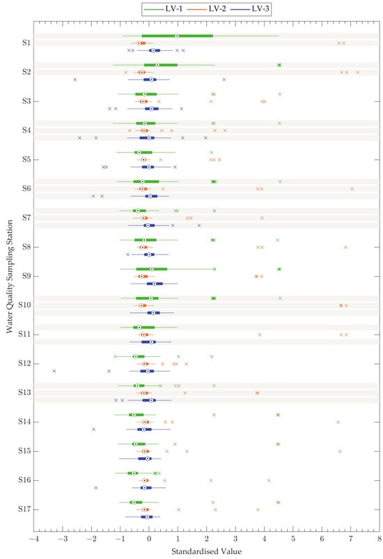
Figure 3.
Spatial variability of latent variables (LVs). The box plot illustrates the distribution of three LVs across 17 water quality sampling stations. The boxes are limited to the 25th and 75th percentiles, and the targets show the median (i.e., 50th percentile) value of the monthly data sets. Whiskers are extended to 1.5 times inter-quartile range to the top and bottom of the boxes. The crosses represent individual outliers for each LV at the respective sampling stations. The shaded LVs at each station are the group identified by cluster analysis (CA) as the highest pollution due to industrial effluents.
The CA grouped the stations almost similarly for all three LVs. Victoria Bridge Station (S1), Kollonnawa Bridge Station (S2), Raggahawatte Ela Station (S4), Maha Ela Station (S6), Pusseli Oya Station (S7), Pugoda Ferry Station (S10), Pugoda Ela station (S11), and Seethawake station (S13) were identified as a distinct group, LV 1. Similarly, except for Pugoda Ela station (S11), the same stations were grouped for LV 2 based on the variations in the LV. For LV 3, Raggahawatte Ela station (S4), Maha Ela station (S6), Pusseli Oya station (S7), Pugoda Ferry station (S10), Pugoda Ela station (S11), and Seethawake station (S13) were grouped into a distinct cluster by the CA.
LV 1 is mainly influenced by Cd and Fe. The average Fe and Cd levels at the 17 stations ranged between 0.32–0.16 mg/L and 0.01–0.04 mg/L, respectively, during the study period (2016–2020) compared to the national water quality standards of 1 mg/L and 0.005 mg/L for Fe and Cd. The stations mentioned above for LV 1 have an exceedance percentage of Category A of the CEA guidelines between 14% and 34% of the time for Fe, and a range of 30% to 32% of the time for Cd. Similarly, nitrate and Pb were the main parameters that contributed to LV 2. The average concentrations at the 17 stations ranged around 0.01 mg/L for Pb and between 0.55 and 1.77 mg/L for nitrate during the study period (2016–2020), compared to the national water quality standard of 0.05 mg/L and 10 mg/L for Pb and nitrate, respectively. Subsequently, the identified stations exceeded Category A of the CEA guidelines within 2% to 6% for nitrate and 1% to 3% for Pb. The highest exceedances were identified at Victoria Bridge (S1) and Maha Ela (S6) stations.
3.2. Industrial Pollution Index (IPI)
A total of six water quality parameters measured at 17 stations over five years were used to develop the IPI. The sub-index was generated using rating curves developed for the six (6) parameters considering the water quality standards imposed by the CEA. The rating curves are shown in Figure 4. For Cd, Fe, and Zn—among the measured parameters—a similar trend was observed, with a significant number of values exceeding the permissible limits specified by the Central Environmental Authority (CEA). As a result, the CEA standard, represented by a red circle, is positioned toward the left side of the graphs for these parameters, indicating a higher rate of exceedance. In contrast, nitrate, Pb, and Cr showed lower percentages of exceedance relative to the standard limits, with the red circle positioned further to the right of the curve. These trends illustrate the pattern of exceedance for each parameter and demonstrate how the percentile-based method effectively identifies the rates of standard limit exceedances for different pollutants.
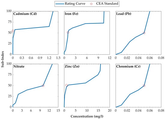
Figure 4.
Rating curves for six water quality parameters. Each curve represents the relationship between the water quality parameter and its sub-index value (Qi,perm). The red circle indicates the standard limit set by the Central Environmental Authority and the assigned sub-index value.
The Random Forest (RF) algorithm was employed to identify the most significant contributing parameters to IPI (i.e., pollution status of the respective parameter), providing a deeper understanding of the six parameters under investigation. The RF model achieved an AUC of 0.98 and an F1-score of 0.99, identifying Cd, Zn, and Fe as the primary parameters influencing river pollution status (Table 4). Then, the ROC method was utilised to calculate the weights for these six parameters. Consistent with the RF model, Cd, Fe, and Zn emerged as the most critical parameters for assessing river water pollution, maintaining the same hierarchical importance identified by the RF model (Table 3).
Table 4.
The relative importance of the six parameters used in the Industrial Pollution Index (IPI).
The final water pollution values were calculated using the five weighted aggregation functions. A sensitivity analysis was conducted, considering all six parameters to identify the best-fitting aggregation function for the changes in sub-index values. The sensitivity analysis results for Fe are shown in Figure 4. The Root Sum Power Function (r = 2) (RSPF 2) and the Root Sum Power Function (r = 4) (RSPF 4) calculated IPI values exceeding the zero (0) to 100 range. Hence, these two functions were not used for the sensitivity analysis. The Weighted Arithmetic Average (WAA) function had better sensitivity than the Weighted Mean Function (WMF) and Weighted Ambiguity and Eclipsity Free Function (WAEFF) functions (Figure 5). The WMF experienced an eclipsing error, failing to produce higher IPI values when the parameter sub-index increased. Conversely, the WAEFF experienced an ambiguity error as it failed to produce lower WPI values when the sub-index values were close to zero. In comparison, the WAA function was free from ambiguity and eclipsing problems. Hence, the WAA function was selected as the best-fitting aggregation function for the developed KRB-IPI.
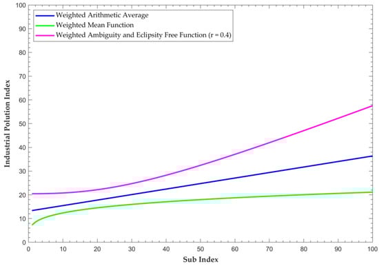
Figure 5.
Results of the sensitivity analysis for iron (Fe).
The LSTM ANN model was developed using the IPI values calculated from the WAA function. About 70% of the calculated index values were used to train the ANN model, and the rest were used for validation. The input variables (X) for the ANN model were the concentrations of the six parameters, while the target variable (Y) was the calculated index value. This model achieved an NSE value of 0.98 and an RMSE value of 0.81, indicating excellent predictive performance, thus validating the consistency of the calculated results of the WAA function (Figure 6). The performance of the LSTM ANN model further suggested that the calculated IPI scores are consistent and free of ambiguity and eclipsing errors.
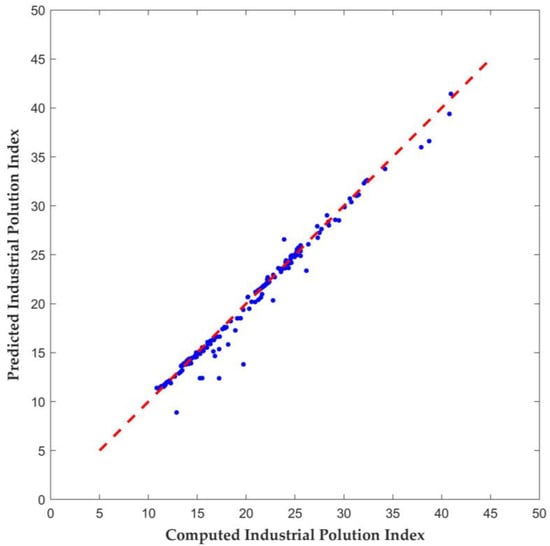
Figure 6.
Calculated vs. predicted (LSTM ANN) of Industrial Pollution Index (IPI) values. The red dashed line represents the line of perfect agreement.
The newly developed KRB-IPI was classified into five categories using the percentile method (Figure 7). This index was then applied to assess the pollution status of the Kelani River across the four monsoon seasons, providing a clearer understanding of the river’s condition (Figure 8). The results suggested that Pugoda Ela (S11), Pusseli Oya (S7), Raggahawatte Ela (S4), and Kollonnawa Bridge (S2) stations experienced high pollution, while the Maha Ela (S6) station was identified with extreme pollution. Nevertheless, comparing water pollution values following the monsoonal patterns of Sri Lanka suggests that the pollution varies during each season. The Maha Ela (S6), Raggahawatte Ela (S4), and Pusseli Oya (S7) stations experienced high and extreme pollution levels year-round, indicating persistent pollution. The Pugoda Ela (S11) and Seethawake Ferry (S13) stations showed significant pollution during the SWM and IM2 periods (Figure 8).
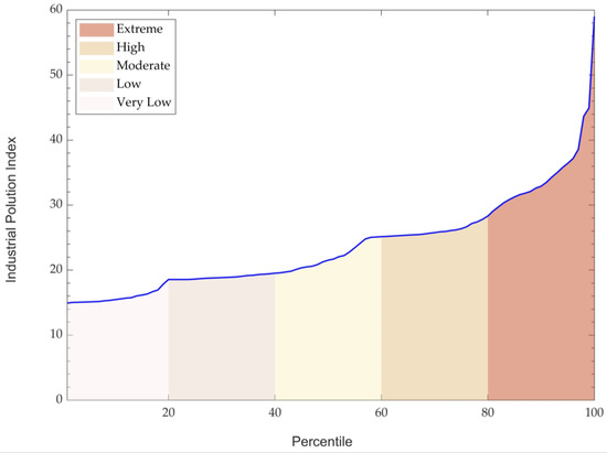
Figure 7.
Classification of the Industrial Pollution Index (IPI) into five categories based on percentile values.
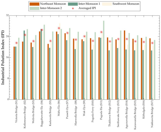
Figure 8.
Seasonal and annual average water pollution scores for the 17 water quality monitoring stations in the Kelani River Basin calculated from the Industrial Pollution Index (IPI).
4. Discussion
In this study, the unsupervised learning (UL) method grouped 17 water quality monitoring stations into two clusters, with one cluster representing stations exhibiting a high exceedance of water quality standards within the basin. The newly developed Industrial Pollution Index (IPI) also identified stations with high and extreme pollution levels in the Kelani River Basin (KRB). The results of the IPI aligned with the cluster, having a high exceedance of water quality standards identified through the UL method. Stations such as Kollonnawa Bridge (S2), Raggahawatte Ela (S4), Maha Ela (S6), Pusseli Oya (S7), and Pugoda Ela (S11) were identified by both methods, highlighting them as key locations with elevated industrial pollutant levels in the KRB.
These identified stations are consistent with findings in the literature. For instance, Pugoda Ela (S11) has experienced significant water quality degradation over the years due to industrial effluents and agricultural runoff [71]. Wastewater generated at INZ1 is discharged into Raggahawatte Canal (S4) [72] and Maha Ela Canal (S6) [73], while the Seethawake station (S13) downstream of the INZ2. The Pusseli Oya (S7) station, situated in a sub-catchment of the KRB, is notably affected by heavy metal pollution [71]. Municipal waste, particularly in Colombo City’s drainage network, also contributes to heavy metal contamination, affecting sites like Kollonnawa Bridge (S2) and Victoria Bridge (S1) [74]. According to previous studies, the Kollonnawa Bridge (S2) station is primarily polluted by municipal and domestic sewage. Thus, the key industrial pollution sources identified in this study include the stations at Maha Ela (S6), Raggahawatte Ela (S4), Pusseli Oya (S7), Pugoda Ferry (S10), Pugoda Ela (S11), and Seethawake Ferry (S13) (Figure 9).
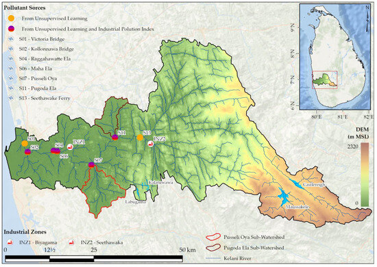
Figure 9.
Identified pollution sources in the Kelani River Basin using the unsupervised learning method and the Industrial Pollution Index method. The topography of the basin (m MSL) was derived from Digital Elevation Model (DEM) data from the Shuttle Radar Topography Mission (SRTM: https://www.earthdata.nasa.gov/sensors/srtm, accessed on 24 May 2024).
In addition to the previously identified stations, the UL method highlighted Seethawake station (S13) as having significant exceedances of standard water quality guidelines. Similarly, the IPI method revealed that pollution levels at Seethawake station increase during periods of heavy rainfall, particularly during the Southwest Monsoon (SWM) and second Inter-monsoon (IM2) seasons. Typically, higher precipitation and streamflow lead to dilution, resulting in lower pollutant concentrations [75]. However, in this case, pollutant levels exceeded standard guidelines more frequently, likely due to surface runoff introducing additional contaminants into the water system. Other stations, such as S4, S6, S7, and S11, classified by the IPI method as having high to extreme water pollution, also exhibited increased pollutant concentrations during the rainy season (Figure 8). This suggests that significant pollutant loads may be released into the water during heavy rainfall, or that runoff is mobilising pollutants from surrounding areas. A similar phenomenon of increasing pollutant levels during rainfall events has been observed in other basins within Sri Lanka [76] as well as in countries with monsoon climates [77]. These findings imply that pollutant discharges into surrounding areas are not adequately regulated by the Central Environmental Authority’s guidelines or the Environmental Protection License scheme, leading to a potential increase in contamination during rainfall events.
The highest exceedance of standard limits was observed for cadmium (Cd) and iron (Fe) using the unsupervised learning approach. Similarly, Cd and Fe also had the highest weighted values in the IPI analysis. This indicates that Cd and Fe are the two primary contributors to the overall pollution status of the Kelani River. Throughout the study period, Cd concentrations exceeded standard limits by 29% to 32% across all 17 stations, while Fe concentrations exceeded limits by 2% to 37%, which explains the moderate pollution scores for most stations, except those identified as key pollutant sources. The frequent exceedance of Cd limits underscores the need for immediate countermeasures, particularly due to the presence of water treatment plants along the Kelani River [37].
5. Conclusions
This study applied machine learning (unsupervised learning) and a novel water pollution index to identify industrial pollution sources in the Kelani River Basin (KRB), Sri Lanka, using six water quality parameters (i.e., Nitrate, Fe, Cd, Cr, Pb, and Zn) from 17 monitoring stations over 2016–2020. Factor Analysis revealed three latent variables, accounting for ~69% of the total variance, with LV 1 (32%) linked to Fe and Cd, LV 2 (20%) to Pb and Nitrate, and LV 3 (17%) to Zn. Cluster analysis identified five key pollution sources. The Industrial Pollution Index (IPI), which was validated using Random Forest (AUC = 0.98, F1-score = 0.99) and an LSTM ANN model (NSE = 0.98, RMSE = 0.81), confirmed four stations as highly polluted and one station as extremely polluted, with Cd levels exceeding limits by 29–32%. These results highlight industrial zones as major contributors to pollution in the Kelani River Basin, Sri Lanka.
While the integrated approach effectively identified pollution sources and is adaptable to other river basins, this study did not consider hydrometeorological factors like precipitation and streamflow, which affect pollutant transport. Future research should integrate these variables, along with advection, dispersion, and diffusion processes, to enhance the accuracy and applicability of the methodology in dynamic environmental conditions.
Author Contributions
Conceptualisation, N.W., L.G., J.B. and J.S.; methodology, L.G and N.W.; software, N.W.; validation, N.W. and L.G.; formal analysis, N.W.; investigation, C.S.P. and H.K.; resources, L.R.; data curation, N.W.; writing—original draft preparation, N.W.; writing—review and editing, L.G., J.B., J.S., L.R., C.S.P. and H.K.; visualisation, N.W. and J.B.; supervision, L.G., J.B., and J.S.; project administration, L.G. and L.R.; All authors have read and agreed to the published version of the manuscript.
Funding
This research received no external funding.
Data Availability Statement
The raw data supporting the conclusions of this article are available from the Central Environmental Authority, Sri Lanka, on request.
Acknowledgments
This study would not have been possible without the support from the Central Environmental Authority, Sri Lanka, freely issuing the data needed in the research, for which the authors are very grateful. The authors are thankful for the generous support extended by the UNESCO-Madanjeet Singh Centre for South Asia Water Management (UMCSAWM), University of Moratuwa.
Conflicts of Interest
The authors declare no conflicts of interest.
Appendix A. Central Environmental Authority Guidelines
The National Environmental Act No. 47 of 1980 is the legislation established by the CEA for protecting and managing the environment in Sri Lanka. The 19th amendment of the act was issued in 2019, and the guidelines for Ambient Water Quality suggested in the guidelines are used as the local guideline to assess inland waterways in Sri Lanka (CEA 2019). The guidelines suggest six categories to assess the water quality. Table A1 shows the guidelines for the water quality parameters identified in the study.
- (1)
- Category A shall be water that requires simple treatment for drinking.
- (2)
- Category B shall be bathing and contact recreational water.
- (3)
- Category C shall be water suitable for aquatic life.
- (4)
- Category D shall be water sources that are required to undergo a general treatment process for drinking.
- (5)
- Category E shall be water suitable for irrigation and agricultural activities.
- (6)
- Category F shall be water with minimum quality but that does not fall into categories A to E
Table A1.
Standard guidelines imposed by the Central Environmental Authority (CEA), Sri Lanka, for the maximum allowable concentrations of industrial pollutants.
Table A1.
Standard guidelines imposed by the Central Environmental Authority (CEA), Sri Lanka, for the maximum allowable concentrations of industrial pollutants.
| Parameter | Category A | Category B | Category C | Category D | Category E | Category F |
|---|---|---|---|---|---|---|
| NO3− as N | 10 | 10 | 10 | 10 | - | 10 |
| Pb | 0.05 | - | 0.002 | 0.05 | - | - |
| Cd | 0.005 | - | 0.005 | 0.005 | - | 5 |
| Fe | 1 | - | - | 2 | - | - |
| Cr | 0.05 | - | 0.02 | 0.05 | - | 0.05 |
| Zn | 1 | - | 1 | 1 | 2 | 24 |
Note: All the concentrations are in mg/L.
References
- WHO. A Global Overview of National Regulations and Standards for Drinking-Water Quality; World Health Organization: Geneva, Switzerland, 2018; ISBN 978-92-4-151376-0. [Google Scholar]
- Wear, S.L.; Acuña, V.; McDonald, R.; Font, C. Sewage Pollution, Declining Ecosystem Health, and Cross-Sector Collaboration. Biol. Conserv. 2021, 255, 109010. [Google Scholar] [CrossRef]
- du Plessis, A. Persistent Degradation: Global Water Quality Challenges and Required Actions. One Earth 2022, 5, 129–131. [Google Scholar] [CrossRef]
- UN-Water. Summary Progress Update 2021: SDG 6—Water and Sanitation for All; UN-Water: Geneva, Switzerland, 2021; pp. 1–58. [Google Scholar]
- Schaffner, M.; Bader, H.P.; Scheidegger, R. Modeling the Contribution of Point Sources and Non-Point Sources to Thachin River Water Pollution. Sci. Total Environ. 2009, 407, 4902–4915. [Google Scholar] [CrossRef] [PubMed]
- Kishor, R.; Purchase, D.; Ferreira, L.F.R.; Mulla, S.I.; Bilal, M.; Bharagava, R.N. Environmental and Health Hazards of Textile Industry Wastewater Pollutants and Its Treatment Approaches. In Handbook of Environmental Materials Management; Springer Nature: Cham, Switzerland, 2020; pp. 1–24. [Google Scholar] [CrossRef]
- Fořt, J.; Kobetičová, K.; Böhm, M.; Podlesný, J.; Jelínková, V.; Vachtlová, M.; Bureš, F.; Černý, R. Environmental Consequences of Rubber Crumb Application: Soil and Water Pollution. Polymers 2022, 14, 1416. [Google Scholar] [CrossRef]
- Anh, N.T.; Can, L.D.; Nhan, N.T.; Schmalz, B.; Luu, T. Le Influences of Key Factors on River Water Quality in Urban and Rural Areas: A Review. Case Stud. Chem. Environ. Eng. 2023, 8, 100424. [Google Scholar] [CrossRef]
- Mawari, G.; Kumar, N.; Sarkar, S.; Frank, A.L.; Daga, M.K.; Singh, M.M.; Joshi, T.K.; Singh, I. Human Health Risk Assessment Due to Heavy Metals in Ground and Surface Water and Association of Diseases with Drinking Water Sources: A Study from Maharashtra, India. Environ. Health Insights 2022, 16, 11786302221146020. [Google Scholar] [CrossRef]
- Ahmed, U.; Mumtaz, R.; Anwar, H.; Shah, A.A.; Irfan, R.; García-Nieto, J. Efficient Water Quality Prediction Using Supervised Machine Learning. Water 2019, 11, 2210. [Google Scholar] [CrossRef]
- Won, H.; Kim, M.; Won, H.; Min, B.; Choi, H. Journal of Hydrology: Regional Studies Machine-Learning-Based Water Quality Management of River with Serial Impoundments in the Republic of Korea. J. Hydrol. Reg. Stud. 2022, 41, 101069. [Google Scholar] [CrossRef]
- Zhu, M.; Wang, J.; Yang, X.; Zhang, Y.; Zhang, L.; Ren, H.; Wu, B.; Ye, L. Eco-Environment & Health A Review of the Application of Machine Learning in Water Quality Evaluation. Eco-Environ. Health 2022, 1, 107–116. [Google Scholar] [CrossRef]
- Buras, M.P.; Solano Donado, F. Identifying and Estimating the Location of Sources of Industrial Pollution in the Sewage Network. Sensors 2021, 21, 3426. [Google Scholar] [CrossRef]
- Xia, F.; Qu, L.; Wang, T.; Luo, L.; Chen, H.; Dahlgren, R.A.; Zhang, M.; Mei, K.; Huang, H. Distribution and Source Analysis of Heavy Metal Pollutants in Sediments of a Rapid Developing Urban River System. Chemosphere 2018, 207, 218–228. [Google Scholar] [CrossRef]
- Wang, L.; Wang, Y.; Xu, C.; An, Z.; Wang, S. Analysis and Evaluation of the Source of Heavy Metals in Water of the River Changjiang. Environ. Monit. Assess. 2011, 173, 301–313. [Google Scholar] [CrossRef] [PubMed]
- Barati Moghaddam, M.; Mazaheri, M.; Mohammad Vali Samani, J. Inverse Modeling of Contaminant Transport for Pollution Source Identification in Surface and Groundwaters: A Review. Groundw. Sustain. Dev. 2021, 15, 100651. [Google Scholar] [CrossRef]
- Prasad, B.; Kumari, P.; Bano, S.; Kumari, S. Ground Water Quality Evaluation near Mining Area and Development of Heavy Metal Pollution Index. Appl. Water Sci. 2014, 4, 11–17. [Google Scholar] [CrossRef]
- Hoseinzadeh, E.; Khorsandi, H.; Wei, C.; Alipour, M. Evaluation of Aydughmush River Water Quality Using the National Sanitation Foundation Water Quality Index (NSFWQI), River Pollution Index (RPI), and Forestry Water Quality Index (FWQI). Desalin. Water Treat. 2015, 54, 2994–3002. [Google Scholar] [CrossRef]
- Karaouzas, I.; Kapetanaki, N.; Mentzafou, A.; Kanellopoulos, T.D.; Skoulikidis, N. Heavy Metal Contamination Status in Greek Surface Waters: A Review with Application and Evaluation of Pollution Indices. Chemosphere 2021, 263, 128192. [Google Scholar] [CrossRef]
- Kumar, A.K.; Sharma, S.; Patel, A.; Dixit, G.; Shah, E. Comprehensive Evaluation of Microalgal Based Dairy Effluent Treatment Process for Clean Water Generation and Other Value Added Products. Int. J. Phytoremediation 2019, 21, 519–530. [Google Scholar] [CrossRef]
- Tiwari, A.K.; Singh, P.K.; Singh, A.K.; De Maio, M. Estimation of Heavy Metal Contamination in Groundwater and Development of a Heavy Metal Pollution Index by Using GIS Technique. Bull. Environ. Contam. Toxicol. 2016, 96, 508–515. [Google Scholar] [CrossRef]
- Brady, J.P.; Ayoko, G.A.; Martens, W.N.; Goonetilleke, A. Development of a Hybrid Pollution Index for Heavy Metals in Marine and Estuarine Sediments. Environ. Monit. Assess. 2015, 187, 306. [Google Scholar] [CrossRef]
- Ouyang, Y.; Nkedi-Kizza, P.; Wu, Q.T.; Shinde, D.; Huang, C.H. Assessment of Seasonal Variations in Surface Water Quality. Water Res. 2006, 40, 3800–3810. [Google Scholar] [CrossRef]
- Zeinalzadeh, K.; Rezaei, E. Determining Spatial and Temporal Changes of Surface Water Quality Using Principal Component Analysis. J. Hydrol. Reg. Stud. 2017, 13, 1–10. [Google Scholar] [CrossRef]
- Aydin, H.; Ustaoğlu, F.; Tepe, Y.; Soylu, E.N. Assessment of Water Quality of Streams in Northeast Turkey by Water Quality Index and Multiple Statistical Methods. Environ. Forensics 2021, 22, 270–287. [Google Scholar] [CrossRef]
- Islam, M.M.; Lenz, O.K.; Azad, A.K.; Ara, M.H.; Rahman, M.; Hassan, N. Assessment of Spatio-Temporal Variations in Water Quality of Shailmari River, Khulna (Bangladesh) Using Multivariate Statistical Techniques. J. Geosci. Environ. Prot. 2017, 5, 1–26. [Google Scholar] [CrossRef]
- Mei, K.; Liao, L.; Zhu, Y.; Lu, P.; Wang, Z.; Dahlgren, R.A.; Zhang, M. Evaluation of Spatial-Temporal Variations and Trends in Surface Water Quality across a Rural-Suburban-Urban Interface. Environ. Sci. Pollut. Res. 2014, 21, 8036–8051. [Google Scholar] [CrossRef] [PubMed]
- Wu, J.; Cheng, S.P.; He, L.Y.; Wang, Y.C.; Yue, Y.; Zeng, H.; Xu, N. Assessing Water Quality in the Pearl River for the Last Decade Based on Clustering: Characteristic, Evolution and Policy Implications. Water Res. 2023, 244, 120492. [Google Scholar] [CrossRef] [PubMed]
- Ustaoğlu, F.; Tepe, Y.; Taş, B. Assessment of Stream Quality and Health Risk in a Subtropical Turkey River System: A Combined Approach Using Statistical Analysis and Water Quality Index. Ecol. Indic. 2020, 113, 105815. [Google Scholar] [CrossRef]
- Alhassan, A.M.; Wan Zainon, W.M.N. Review of Feature Selection, Dimensionality Reduction and Classification for Chronic Disease Diagnosis. IEEE Access 2021, 9, 87310–87317. [Google Scholar] [CrossRef]
- Govender, P.; Sivakumar, V. Application of K-Means and Hierarchical Clustering Techniques for Analysis of Air Pollution: A Review (1980–2019). Atmos. Pollut. Res. 2020, 11, 40–56. [Google Scholar] [CrossRef]
- Badillo, S.; Banfai, B.; Birzele, F.; Davydov, I.I.; Hutchinson, L.; Kam-Thong, T.; Siebourg-Polster, J.; Steiert, B.; Zhang, J.D. An Introduction to Machine Learning. Clin. Pharmacol. Ther. 2020, 107, 871–885. [Google Scholar] [CrossRef] [PubMed]
- Topp, S.N.; Pavelsky, T.M.; Jensen, D.; Simard, M.; Ross, M.R.V. Research Trends in the Use of Remote Sensing for Inland Water Quality Science: Moving towards Multidisciplinary Applications. Water 2020, 12, 169. [Google Scholar] [CrossRef]
- Madhav, S.; Ahamad, A.; Singh, A.K.; Kushawaha, J.; Chauhan, J.S.; Sharma, S.; Singh, P. Water Pollutants: Sources and Impact on the Environment and Human Health. In Sensors in Water Pollutants Monitoring: Role of Material; Springer: Berlin/Heidelberg, Germany, 2020; pp. 43–62. [Google Scholar] [CrossRef]
- Mahaweli Authority of Sri Lanka. Annual Report 2017; Ministry of Mahaweli Development and Environment: Colombo, Sri Lanka, 2017.
- Mahagamage, M.G.Y.L.; Manage, P.M. Water Quality Index (CCME-WQI) Based Assessment Study of Water Quality in Kelani River Basin, Sri Lanka. Int. J. Environ. Nat. Resour. 2014, 1, 199–204. [Google Scholar]
- Narangoda, C.; Amarathunga, D.; Dangalle, C.D. Evaluation of Water Quality in the Upper and Lower Catchments of the Kelani River Basin, Sri Lanka. Water Pract. Technol. 2023, 18, 716–737. [Google Scholar] [CrossRef]
- United Nations (UN). World Population Prospects 2024; United Nations: New York, NY, USA, 2024; ISBN 978-92-1-148373-4. [Google Scholar]
- Manage, P.; Mahagamage, Y.L.; Ajward, R.; Amaratunge, S.; Amarathunga, V.I. The Need for Proper Management Leading to the Sustainability of the Kelani River and Its Lower Basin. J. Water Land Dev. 2020, 47, 10–15. [Google Scholar] [CrossRef]
- Central Environmental Authority. Annual Report 2021; Central Environmental Authority: Colombo, Sri Lanka, 2021. [Google Scholar]
- Hemachandra, C.K.; Pathiratne, A. Assessing Toxicity of Two Industrial Zone Effluents Reaching Kelani River, Sri Lanka. J. Natl. Sci. Found. Sri Lanka 2018, 46, 539–546. [Google Scholar] [CrossRef]
- Azam, H.M.; Alam, S.T.; Hasan, M.; Yameogo, D.D.S.; Kannan, A.D.; Rahman, A.; Kwon, M.J. Phosphorous in the Environment: Characteristics with Distribution and Effects, Removal Mechanisms, Treatment Technologies, and Factors Affecting Recovery as Minerals in Natural and Engineered Systems. Environ. Sci. Pollut. Res. 2019, 26, 20183–20207. [Google Scholar] [CrossRef] [PubMed]
- Shrestha, N. Factor Analysis as a Tool for Survey Analysis. Am. J. Appl. Math. Stat. 2021, 9, 4–11. [Google Scholar] [CrossRef]
- Asuero, A.G.; Sayago, A.; González, A.G. The Correlation Coefficient: An Overview. Crit. Rev. Anal. Chem. 2006, 36, 41–59. [Google Scholar] [CrossRef]
- Zakaria, M.; Al-Shebany, M.; Sarhan, S. Artificial Neural Network: A Brief Overview. J. Eng. Res. Appl. 2014, 4, 7–12. [Google Scholar]
- Treshansky, A.; McGraw, R.M. Overview of Clustering Algorithms. Enabling Technol. Simul. Sci. V 2001, 4367, 41. [Google Scholar] [CrossRef]
- Omran, M.G.H.; Engelbrecht, A.P.; Salman, A. An Overview of Clustering Methods. Intell. Data Anal. 2007, 11, 583–605. [Google Scholar] [CrossRef]
- Lukhabi, D.K.; Mensah, P.K.; Asare, N.K.; Pulumuka-Kamanga, T.; Ouma, K.O. Adapted Water Quality Indices: Limitations and Potential for Water Quality Monitoring in Africa. Water 2023, 15, 1736. [Google Scholar] [CrossRef]
- Kumar, D.; Alappat, B.J. Selection of the Appropriate Aggregation Function for Calculating Leachate Pollution Index. Pract. Period. Hazard. Toxic Radioact. Waste Manag. 2004, 8, 253–264. [Google Scholar] [CrossRef]
- Chidiac, S.; El Najjar, P.; Ouaini, N.; El Rayess, Y.; El Azzi, D. A Comprehensive Review of Water Quality Indices (WQIs): History, Models, Attempts and Perspectives; Springer: Dordrecht, The Netherlands, 2023; Volume 22, ISBN 0123456789. [Google Scholar]
- Hallock, D. A Water Quality Index for Ecology’s Stream Monitoring Program; Washington State Department of Ecology: Olympia, Greece, 2002.
- Casillas-García, L.F.; de Anda, J.; Yebra-Montes, C.; Shear, H.; Díaz-Vázquez, D.; Gradilla-Hernández, M.S. Development of a Specific Water Quality Index for the Protection of Aquatic Life of a Highly Polluted Urban River. Ecol. Indic. 2021, 129, 107899. [Google Scholar] [CrossRef]
- Uddin, M.G.; Rahman, A.; Nash, S.; Diganta, M.T.M.; Sajib, A.M.; Moniruzzaman, M.; Olbert, A.I. Marine Waters Assessment Using Improved Water Quality Model Incorporating Machine Learning Approaches. J. Environ. Manag. 2023, 344, 118368. [Google Scholar] [CrossRef] [PubMed]
- Gaya, M.S.; Abba, S.I.; Abdu, A.M.; Tukur, A.I.; Saleh, M.A.; Esmaili, P.; Wahab, N.A. Estimation of Water Quality Index Using Artificial Intelligence Approaches and Multi-Linear Regression. IAES Int. J. Artif. Intell. 2020, 9, 126–134. [Google Scholar] [CrossRef]
- Xiong, Y.; Zhang, T.; Sun, X.; Yuan, W.; Gao, M.; Wu, J.; Han, Z. Groundwater Quality Assessment Based on the Random Forest Water Quality Index—Taking Karamay City as an Example. Sustainability 2023, 15, 14477. [Google Scholar] [CrossRef]
- Uddin, M.G.; Nash, S.; Rahman, A.; Olbert, A.I. Development of a Water Quality Index Model—A Comparative Analysis of Various Weighting Methods. In Proceedings of the Mediterranean Geosciences Union Annual Meeting, Instanbul, Turkey, 25–28 November 2021; pp. 1–6. [Google Scholar]
- Xu, J.; Xu, Z.; Kuang, J.; Lin, C.; Xiao, L.; Huang, X.; Zhang, Y. An Alternative to Laboratory Testing: Random Forest-Based Water Bodies. Water 2021, 13, 3626. [Google Scholar] [CrossRef]
- Salman, H.A.; Kalakech, A.; Steiti, A. Random Forest Algorithm Overview. Babylon. J. Mach. Learn. 2024, 2014, 69–79. [Google Scholar] [CrossRef]
- Biau, G.; Scornet, E. A Random Forest Guided Tour. Test 2016, 25, 197–227. [Google Scholar] [CrossRef]
- Varshney, T.; Waghmare, A.V.; Singh, V.P.; Ramu, M.; Patnana, N.; Meena, V.P.; Azar, A.T.; Hameed, I.A. Investigation of Rank Order Centroid Method for Optimal Generation Control. Sci. Rep. 2024, 14, 11267. [Google Scholar] [CrossRef]
- Syeed, M.M.M.; Hossain, M.S.; Karim, M.R.; Uddin, M.F.; Hasan, M.; Khan, R.H. Surface Water Quality Profiling Using the Water Quality Index, Pollution Index, and Statistical Methods: A Critical Review. Environ. Sustain. Indic. 2023, 18, 100247. [Google Scholar] [CrossRef]
- Akhtar, N.; Ishak, M.I.S.; Ahmad, M.I.; Umar, K.; Md Yusuff, M.S.; Anees, M.T.; Qadir, A.; Almanasir, Y.K.A. Modification of the Water Quality Index (Wqi) Process for Simple Calculation Using the Multi-Criteria Decision-Making (Mcdm) Method: A Review. Water 2021, 13, 905. [Google Scholar] [CrossRef]
- Uddin, M.G.; Nash, S.; Olbert, A.I. A Review of Water Quality Index Models and Their Use for Assessing Surface Water Quality. Ecol. Indic. 2021, 122, 107218. [Google Scholar] [CrossRef]
- Khouri, L.; Bashar Al-Moufti, M. Selection of Suitable Aggregation Function for Estimation of Water Quality Index for the Orontes River. Ecol. Indic. 2022, 142, 109290. [Google Scholar] [CrossRef]
- Shen, C. A Transdisciplinary Review of Deep Learning Research and Its Relevance for Water Resources Scientists. Water Resour. Res. 2018, 54, 8558–8593. [Google Scholar] [CrossRef]
- Han, K.; Wang, Y. A Review of Artificial Neural Network Techniques for Environmental Issues Prediction. J. Therm. Anal. Calorim. 2021, 145, 2191–2207. [Google Scholar] [CrossRef]
- Jaffar, A.; Thamrin, N.M.; Ali, M.S.A.M.; Misnan, M.F.; Yassin, A.I.M. Water Quality Prediction Using Lstm-Rnn: A Review. J. Sustain. Sci. Manag. 2022, 17, 204–225. [Google Scholar] [CrossRef]
- Bayissa, Y.A.; Tadesse, T.; Svoboda, M.; Wardlow, B.; Poulsen, C.; Swigart, J.; Van Andel, S.J. Developing a Satellite-Based Combined Drought Indicator to Monitor Agricultural Drought: A Case Study for Ethiopia. GIScience Remote Sens. 2019, 56, 718–748. [Google Scholar] [CrossRef]
- Agrawal, N.; Dixit, J. Assessment of Landslide Susceptibility for Meghalaya (India) Using Bivariate (Frequency Ratio and Shannon Entropy) and Multi-Criteria Decision Analysis (AHP and Fuzzy-AHP) Models. All Earth 2022, 34, 179–201. [Google Scholar] [CrossRef]
- Ritter, A.; Muñoz-Carpena, R. Performance Evaluation of Hydrological Models: Statistical Significance for Reducing Subjectivity in Goodness-of-Fit Assessments. J. Hydrol. 2013, 480, 33–45. [Google Scholar] [CrossRef]
- Makubura, R.; Meddage, D.P.P.; Azamathulla, H.M.; Pandey, M.; Rathnayake, U. A Simplified Mathematical Formulation for Water Quality Index (WQI): A Case Study in the Kelani River Basin, Sri Lanka. Fluids 2022, 7, 147. [Google Scholar] [CrossRef]
- Gunawardana, M.H.M.A.S.V.; Sanjaya, K.; Atapaththu, K.S.S.; Yapa Mudiyanselage, A.L.W.Y.; Masakorala, K.; Widana Gamage, S.M.K. Quantitative Prediction of Toxin-Producing Aphanizomenon Cyanobacteria in Freshwaters Using Sentinel-2 Satellite Imagery. J. Water Health 2022, 20, 1364–1379. [Google Scholar] [CrossRef] [PubMed]
- Ruvinda, K.M.; Pathiratne, A. Biomarker Responses of Nile Tilapia (Oreochromis niloticus) Exposed to Polluted Water from Kelani River Basin, Sri Lanka: Implications for Biomonitoring River Pollution. Sri Lanka J. Aquat. Sci. 2018, 23, 105. [Google Scholar] [CrossRef][Green Version]
- Ranasinghe, P.N.; Siriwardana, Y.P.S.; Wanasinghe, V.R. Heavy Metal Pollution in Drainage Network of Colombo City and Suburbs of Sri Lanka. Chin. J. Geochem. 2006, 25, 84–85. [Google Scholar] [CrossRef]
- Xu, G.; Li, P.; Lu, K.; Tantai, Z.; Zhang, J.; Ren, Z.; Wang, X. Catena Seasonal Changes in Water Quality and Its Main in Fl Uencing Factors in the Dan River Basin. Catena 2019, 173, 131–140. [Google Scholar] [CrossRef]
- Diwyanjalee, G.R.; Premarathne, W.A.P.J. Impact of Rainfall on the Water Quality of a Tropical River: Based on the Nilwala River in the Southern Province of Sri Lanka between March and October 2019. Water Pract. Technol. 2024, 19, 2352–2363. [Google Scholar] [CrossRef]
- Tuan, A.; Babel, S. Science of the Total Environment Microplastics and Heavy Metals in a Tropical River: Understanding Spatial and Seasonal Trends and Developing Response Strategies Using DPSIR Framework. Sci. Total Environ. 2024, 897, 165405. [Google Scholar] [CrossRef]


Disclaimer/Publisher’s Note: The statements, opinions and data contained in all publications are solely those of the individual author(s) and contributor(s) and not of MDPI and/or the editor(s). MDPI and/or the editor(s) disclaim responsibility for any injury to people or property resulting from any ideas, methods, instructions or products referred to in the content. |
© 2024 by the authors. Licensee MDPI, Basel, Switzerland. This article is an open access article distributed under the terms and conditions of the Creative Commons Attribution (CC BY) license (https://creativecommons.org/licenses/by/4.0/).