Research on Strategies for Controlling Cross-Border Water Pollution under Different Management Scenarios

Abstract

The issue of water pollution in river basins poses a serious threat to the economic development of upstream and downstream regions. We have compared the water pollution control inputs and benefits of upstream and downstream governments under different management scenarios: non-cooperation, cooperation, and basin agency-led cooperation. The results show that the basin agency-led cooperation has achieved remarkable results, significantly reducing water pollution emissions, increasing input in treatment, and thereby maximizing the overall benefits of the basin. As the cost of water pollution damage rises, while the initial increase in water pollution control investment may temporarily compress the total basin income, the improvement in water quality eventually leads to a rebound in total benefit, highlighting the critical role of collaborative governance and basin-level management. The study emphasizes that establishing a collaborative governance system for river basins is crucial. It can facilitate close cooperation and resource sharing between upstream and downstream regions, optimizing water pollution control efforts and promoting sustainable economic development within the basin.

1. Introduction

With the rapid development of industrialization, urbanization and transport, the problem of pollution in basins has become increasingly serious [1]. Water is a fundamental natural resource necessary for the survival and development of human societies, and water scarcity can greatly threaten the process of sustainable development in all countries [2]. The externalities and non-exclusivity of the basin environment as a public good have led to the emergence of the “tragedy of the commons” [3,4]. Some local governments have adopted “free rider” behaviors, shifting water pollution problems to other regions, choosing not to bear or bear less responsibility for water pollution control, relying on the efforts of other entities to maximize their own interests, increasing the environmental burden and posing a potential threat to the global ecosystem [5]. With China’s increasing attention to ecological environment, the State Council has proposed a new direction for the governance of river pollution, namely the principle of beneficiary pays. In order to enhance environmental quality and social welfare, local governments have implemented various environmental policies, such as emission taxes and increased input in water pollution control, to effectively regulate and reduce water pollution occurrence and spread [6,7]. The control of watershed water pollution is primarily government-oriented, relying on policies such as government environmental investment policies, command-and-control policies, and ecological compensation policies [8]. Cross-border water pollution management faces challenges, and there is a need to balance the costs and benefits between different regions to ensure that management is comprehensive and sustainable [9].

For research on water pollution control, Lu and Yu [10] investigated the pollutant emissions and regional pollution sources in cross-border river basins, analyzed their spatiotemporal characteristics, and established a comprehensive predictive model. El Ouardighi, et al. [11] used a non-cooperation two-stage game model to study the trade-off between double marginalization on pollution discharge and abatement efforts. Guo and Duan [12] used a computer-based simulation system to ascertain the scope of environmental harm resulting from water pollution events. Furthermore, its scientific reliability was corroborated through practical instances. Regional cooperation has become a popular means of managing shared resources and resolving cross-jurisdictional boundary issues. Jing, et al. [13] evaluated the effectiveness of China’s cross-border water pollution joint governance policy and emphasized the importance of cooperation between upstream and downstream regions. Jiang, et al. [14] analyzed the cross-border pollution control problem using a stochastic differential game model, and the results showed that cross-regional cooperation is more effective than non-cooperation in solving environmental challenges. Benchekroun and Martín-Herrán [15] investigated the impact of the relationship between emissions and future pollution levels in the cross-border pollution game.

In terms of formulating environmental policies, Bellver-Domingo, et al. [16] argued that ecological compensation can internalize the socio-economic and environmental costs of implementing policies. Jiang and You [17] established a horizontal ecological compensation mechanism to balance the losses in cross-border governance cooperation through local compensation-based and central financial support. Hao, et al. [18] proposed a method for calculating ecological compensation standards for cross-border river basins based on water allocation and water quality control objectives. Li [19,20] found the non-cooperation and cooperation optimal emission paths for two regions by considering emission permit trading using optimal control theory. Huang [21] evaluated the effectiveness of combining pollution taxes with pollution control in basin environmental management and highlighted the importance of cooperation between upstream and downstream regions in addressing cross-border water pollution, shedding light on the dynamic changes in environmental and social welfare under pollution governance cooperation and ecological compensation mechanisms. Chang, et al. [22] considered learning by doing in addition to the existing framework. Zhao, et al. [23] proposed a transfer tax model that considers the geographic structure of the basin, reducing the cost of pollution abatement across the basin by determining the optimal transfer tax rate. Song and Wu [24] devised a game model to study stochastic water quality variations. It integrates “water quality currency” transactions by pollution control firms, examining their interplay with pollution control efforts. Sheng and Webber [25] examined the influence of local actors in cross-border water pollution control and proposed incentive coordination as an effective solution that can contribute to water quality improvement. Kolaolusanya, et al. [26] found that most people were aware of water pollution and prevention strategies, but had poor attitudes toward water conservation. Jia, et al. [27] evaluated pollution control issues concerning neighboring local governments and the central government and found that subsidies from the central government can incentivize local governments to actively address pollution.

These studies have taken into account a variety of approaches, including regional cooperation, ecological compensation, optimal control theory, transfer tax modeling and new trading mechanisms, and have provided extensive theoretical support and policy recommendations for solving cross-border water pollution problems. In the realm of research on cross-border water pollution governance, scholars tend to concentrate on either a single management strategy or an isolated analysis of cooperation and non-cooperation mechanisms between regions. However, few studies have comprehensively and systematically examined the three distinct strategic modes of non-cooperation, cooperation, and basin agency-led cooperation, while also exploring the introduction of cost-sharing contracts within the framework of cooperative strategies. Furthermore, given the regional characteristics of water pollution issues, where the discharge of pollutants from upstream areas inevitably causes environmental damage and economic losses to downstream areas, this reality necessitates its incorporation into research designs. Therefore, this paper researches and explores the management mechanisms under different management scenarios. This paper systematically examines the decision-making of upstream and downstream governments under non-cooperation, cooperation and basin agency-led cooperation scenarios, and provides an in-depth analysis of their optimal inputs and optimal emission strategies in pollution management, taking the pollution management inputs from basin agencies to upstream and downstream regional governments as the object of the study. Notably, in the cooperation scenario, this study also introduces the concept of cost-sharing contracts to promote cooperation between upstream and downstream in pollution management.

The rest of the paper is organized as follows: in Section 2, the notation and basic assumptions of the model are constructed. In Section 3, the models are constructed for decision-making under the non-cooperation scenario, the cooperation scenario, and the basin agency-led cooperation scenario, and the optimal pollution emissions and pollution control inputs are obtained. Section 4 compares and analyzes the pollution control strategies under different scenarios, and further examines the emission reduction input efficiency and damage cost against the optimal strategy through the arithmetic example subsection. Finally, Section 5 summarizes the full paper.

2. Model Notation and Basic Assumptions

This paper investigates the optimal water pollution control inputs and emissions for upstream local governments (U) and downstream local governments (D) under three management scenarios. Regional administrations upstream and downstream are rational, and in order to minimize the environmental damage caused by water pollution, regional administrations upstream and downstream will invest in water pollution control. Consider three scenarios of water pollution control: (1) in the non-cooperation scenario, the regional administrations upstream and downstream carry out water pollution control separately, independently decide on the input in water pollution control, and pursue their own revenue maximization; (2) in the cooperation scenario, since upstream local governments will benefit downstream local governments by treating water pollution in their regions, downstream regions will incentivize more water pollution control inputs by sharing the cost of water pollution control inputs in upstream regions through cost-sharing contracts; (3) in the basin agency-led cooperation scenario, where the upstream and downstream regions make decisions to maximize the benefits of the basin as a whole. The equilibrium strategies of regional administrations upstream and downstream under the three scenarios are brought to the solution analysis. The main notation is illustrated in

Table 1. Meaning of model parameters.

Parameter	Meaning
$e_i$	Pollutant emission load from industry in upstream and downstream areas, where $i=U,D$
$I_i$	Upstream and downstream water pollution control inputs, where $i=U,D$
${\gamma }_i$	Cost coefficients of regional administrations upstream and downstream for water pollution control, where $i=U,D$
$\delta$	Natural decomposition rate of pollutants
${\mu }_i$	Unit emission reduction input efficiency, which measures the amount of pollutant emissions that can be reduced per unit of water pollution control inputs, where $i=U,D$
$d_i$	The degree of damage per unit of pollutant suffered by the region, where $i=U,D$

.

Assuming that the emissions of pollutants from industrial firms in the basin area are linearly related to industrial output, the two regions can generate a certain amount of revenue from industrial production, so that the revenue from industrial output can be expressed as a function of emissions. Meanwhile, the revenue function is a quadratic increasing convex function of emissions, indicating that pollutant emissions are taken when the production yield is maximized, and the regional yield increases with pollutant emissions. Drawing on the classical model of Jørgensen and Zaccour [28], the revenue function of the region can be carved out, where the yield factor $b_i$ satisfies $0\le e_i\le b_i$,

$$e_i(b_i-{\displaystyle \frac{1}{2}}{e}_i),$$

(1)

The regional administrations upstream and downstream need water pollution control input costs, such as water pollution control and public environmental protection awareness, in addition to production activities for basin water pollution control [29,30]. It is assumed that the regional administrations upstream and downstream water pollution control cost inputs are $C_i$, where $i=U,D$:

$$C_i={\displaystyle \frac{{\gamma }_i}{2}}{I}_i^2,$$

(2)

The actual emissions of pollutants in the basin are related to the upstream and downstream local government’s input in water pollution control and are also affected by the natural attenuation rate of pollutants. Assuming that the reduction of pollutants in the basin is linear in terms of financial inputs, the actual emissions of water pollution $R_i$ in the region $i$, $i=U,D$ can be expressed as follows:

$$R_i=(1-\delta )e_i-{\mu }_i{I}_i,$$

(3)

Assuming that water pollution in a river basin is caused by mixed pollutants, it primarily exerts a regional impact on both the local area and adjacent regions. Pollutant emissions cause damage to upstream and downstream regional waters, with damage costs depending on actual emissions, and assuming that damage costs to the region $i$, $i=U,D$ are linear, can be expressed as follows:

$$D_i=d_i{\sum }_{k=1}^2{R}_k,$$

(4)

Therefore, the objective function under the non-negativity constraint in upstream and downstream $i$, $i=U,D$ areas is constructed as follows:

$$\mathit{max}{W}_i=e_i\left(b_i-{\displaystyle \frac{1}{2}}{e}_i\right)-{\displaystyle \frac{{\gamma }_i}{2}}{I}_i^2-d_i{\sum }_{k=1}^2{R}_k,$$

$$\mathrm{s}.\mathrm{t}.(1-\delta )e_i-\mu I_i\ge 0,$$

(5)

3. Model Modeling and Solution Analysis

In order to better investigate the impact of upstream and downstream areas governing the water basin environment under different management scenarios, this paper examines and analyzes upstream and downstream government decision-making under a non-cooperation scenario, a cooperation scenario, and a basin agency-led cooperation scenario.

3.1. Non-Cooperation Scenario

In the non-cooperation scenario, the decision-making processes of regional administrations upstream and downstream are independent and simultaneous. The objectives of upstream and downstream governments are to find the optimal water pollution control input strategies to maximize their respective benefits. ${W_i}^N$ denotes the benefits of upstream and downstream governments in the non-cooperation scenario, and the equilibrium outcomes of upstream and downstream governments in the non-cooperation scenario are distinguished by the superscript $“N”.$ Therefore, the profit functions of regional administrations upstream and downstream under the non-cooperation scenario are given by the following:

$$\mathit{max}{W_U}^N=e_U\left(b_U-{\displaystyle \frac{1}{2}}{e}_U\right)-{\displaystyle \frac{{\gamma }_U}{2}}{I}_U^2-d_U{R}_U,$$

$$\mathrm{s}.\mathrm{t}.(1-\delta )e_U-{\mu }_U{I}_U\ge 0,$$

(6)

$$\mathit{max}{W_D}^N=e_D\left(b_D-{\displaystyle \frac{1}{2}}{e}_D\right)-{\displaystyle \frac{{\gamma }_D}{2}}{I}_D^2-d_D\left(R_U+R_D\right),$$

$$\mathrm{s}.\mathrm{t}.(1-\delta )e_D-{\mu }_D{I}_D\ge 0,$$

(7)

Theorem 1.

Feedback equilibrium in the non-cooperation scenario:

(1) The optimal solution for pollutant emissions and water pollution control inputs in the upstream region is as follows:

$$\left({e_U}^N, {I_U}^N\right)=\left\{\begin{array}{ll}\left(b_U-d_U\left(1-\delta \right), {\displaystyle \frac{{\mu }_U}{{\gamma }_U}}{d}_U\right)& R_U>0\\ ({\displaystyle \frac{{{\mu }_U}^2{b}_U}{{\left(1-\delta \right)}^2{\gamma }_U+{{\mu }_U}^2}}, {\displaystyle \frac{\left(1-\delta \right){\mu }_U{b}_U}{{\left(1-\delta \right)}^2{\gamma }_U+{{\mu }_U}^2}})& R_U=0\end{array},\right.$$

(8)

(2) The optimal solution for pollutant emissions and water pollution control inputs in the downstream region is as follows:

$$\left({e_D}^N, {I_D}^N\right)=\left\{\begin{array}{ll}\left(b_D-d_D\left(1-\delta \right), {\displaystyle \frac{{\mu }_D}{{\gamma }_D}}{d}_D\right)& R_D>0\\ ({\displaystyle \frac{{{\mu }_D}^2{b}_D}{{\left(1-\delta \right)}^2{\gamma }_D+{{\mu }_D}^2}}, {\displaystyle \frac{\left(1-\delta \right){\mu }_D{b}_D}{{\left(1-\delta \right)}^2{\gamma }_D+{{\mu }_D}^2}})& R_D=0\end{array},\right.$$

(9)

Proof of Theorem 1.

See Appendix A for proof. □

Theorem 1 shows that in the non-cooperation scenario, the optimal water pollution control inputs of upstream and downstream governments are positively correlated with both the sensitivity coefficient of pollutant emissions to local inputs and the degree of damage per unit of pollutant suffered by the region. Conversely, the degree of damage per unit of pollutant suffered by the region is negatively correlated with the emissions of pollutants, and the water pollution control inputs are negatively correlated with the coefficient of water pollution control costs. This indicates that upstream and downstream governments should consider the cost of water pollution control to promote the reduction of pollutants as well as to bring their own benefits to determine the optimal amount of water pollution control inputs in the river basin. In the non-cooperation scenario, both upstream and downstream governments maximize their own benefits without considering the interests of the basin as a whole.

3.2. Cooperation Scenario

In the cooperation scenario, the downstream local governments share the water pollution control costs of the upstream local governments in order to incentivize them to increase their input in water pollution, and thus, further increase their incentives to address water pollution, with a cost-sharing ratio of $\alpha$. In this way, the regional administrations upstream and downstream form a Stackelberg game model in which the downstream government is the leader, and the downstream government is the follower. ${W_i}^S$ denotes the benefit of region i in the cooperation scenario, and the equilibrium results of each region under the consideration of cost-sharing decision are distinguished by “$S$” as a superscript. Therefore, under the cooperation scenario, the objective functions of regional administrations upstream and downstream are as follows:

$$\mathit{max}{W_U}^S=e_U\left(b_U-{\displaystyle \frac{1}{2}}{e}_U\right)-\left(1-\alpha \right){\displaystyle \frac{{\gamma }_U}{2}}{I}_U^2-d_U{R}_U,$$

$$\mathrm{s}.\mathrm{t}.(1-\delta )e_U-{\mu }_U{I}_U\ge 0,$$

(10)

$$\mathit{max}{W_D}^N=e_D\left(b_D-{\displaystyle \frac{1}{2}}{e}_D\right)-{\displaystyle \frac{{\gamma }_D}{2}}{I}_D^2-d_D\left(R_U+R_D\right)-\alpha {\displaystyle \frac{{\gamma }_U}{2}}{I}_U^2,$$

$$\mathrm{s}.\mathrm{t}.(1-\delta )e_D-{\mu }_D{I}_D\ge 0,$$

(11)

Theorem 2.

Feedback equilibrium in cooperation scenario:

(1) The optimal solution for pollutant emissions and water pollution control inputs in the upstream region is as follows:

$$\left({e_U}^S, {I_U}^S\right)=\left\{\begin{array}{ll}\left(b_U-d_U\left(1-\delta \right), {\displaystyle \frac{{\mu }_U{d}_U}{\left(1-\alpha \right){\gamma }_U}}\right)& R_U>0\\ ({\displaystyle \frac{{\mu }_U^2{b}_U}{\left(1-\alpha \right){\left(1-\delta \right)}^2{\gamma }_U+{{\mu }_U}^2}}, {\displaystyle \frac{\left(1-\delta \right){\mu }_U{b}_U}{\left(1-\alpha \right){\left(1-\delta \right)}^2{\gamma }_U+{{\mu }_U}^2}})& R_U=0\end{array},\right.$$

(12)

(2) The optimal solution for pollutant emissions and water pollution control inputs in the downstream region is as follows:

$$\left({e_D}^S, {I_D}^S\right)=\left\{\begin{array}{ll}\left(b_D-d_D\left(1-\delta \right), {\displaystyle \frac{{\mu }_D}{{\gamma }_D}}{d}_D\right)& R_D>0\\ ({\displaystyle \frac{{{\mu }_D}^2{b}_D}{{\left(1-\delta \right)}^2{\gamma }_D+{{\mu }_D}^2}}, {\displaystyle \frac{\left(1-\delta \right){\mu }_D{b}_D}{{\left(1-\delta \right)}^2{\gamma }_D+{{\mu }_D}^2}})& R_D=0\end{array},\right.$$

(13)

(3) The proportion of the downstream region’s share of the water pollution control cost to the upstream local government is as follows:

$$\mathsf{\alpha }=1-{\displaystyle \frac{d_U}{2d_D}},$$

(14)

Proof of Theorem 2.

See Appendix B for proof. □

From Theorem 2, under the cooperation scenario, when the upstream and downstream regions actually have water pollution emissions, the optimal water pollution control inputs are positively related to both the sensitivity coefficients of the pollutant emissions to the local inputs, and the degree of damage per unit of pollutant suffered by the region; whereas the degree of damage per unit of pollutant suffered by the region is negatively related to the emissions of pollutants, and the water pollution control inputs are negatively related to the coefficients of the water pollution control costs. At the same time, the optimal water pollution control inputs of the upstream region are positively related to the downstream cost-sharing ratio. The upstream and downstream governments still make decisions based on their own revenue maximization, but cost sharing from the downstream government to the upstream government can promote the upstream government’s efforts to increase water pollution control inputs. The cost-sharing coefficient of downstream regions to upstream regions is related to the degree of damage per unit of pollutant suffered by upstream and downstream regions, and downstream governments will share costs with upstream regions only if they fulfill certain conditions, that is, $2d_D>d_U$.

3.3. Basin Agency-Led Cooperation Scenario

In the basin agency-led cooperation scenario, regional administrations upstream and downstream do not only consider their own benefits but also make decisions with the goal of maximizing the benefits of the basin as a whole. $W^C$ denotes the benefit of region i under the cooperation scenario led by the basin agency, and the equilibrium results of each region under the cooperation scenario led by the basin agency are distinguished by “$C$” as the superscript. The decision-making objective function at this point is as follows:

$$\mathit{max}{W}^C=e_U\left(b_U-{\displaystyle \frac{1}{2}}{e}_U\right)+e_D\left(b_D-{\displaystyle \frac{1}{2}}{e}_D\right)-{\displaystyle \frac{{\gamma }_U}{2}}{I}_U^2-{\displaystyle \frac{{\gamma }_D}{2}}{I}_D^2-\left(d_U+d_D\right)R_U-d_D{R}_D$$

$$\mathrm{s}.\mathrm{t}.\left(1-\mathsf{\delta }\right){\mathrm{e}}_{\mathrm{U}}-{\mathsf{\mu }}_{\mathrm{U}}{\mathrm{I}}_{\mathrm{U}}\ge 0, \left(1-\mathsf{\delta }\right){\mathrm{e}}_{\mathrm{D}}-{\mathsf{\mu }}_{\mathrm{D}}{\mathrm{I}}_{\mathrm{D}}\ge 0,$$

(15)

Theorem 3.

Feedback equilibrium in the basin agency-led cooperation scenario. The optimal solutions for upstream and downstream governments’ pollutant emissions and water pollution control inputs are as follows:

$$\left\{\left({e_U}^C, {I_U}^C\right), \left({e_D}^C, {I_D}^C\right)\right\}=\left\{\begin{array}{l}\begin{array}{cc}\left(b_U-(d_U+d_D)(1-\delta ), {\displaystyle \frac{{\mu }_U(d_U+d_D)}{{\gamma }_U}}\right), \left(b_D-d_D(1-\delta ), {\displaystyle \frac{{\mu }_D{d}_D}{{\gamma }_D}}\right)& \hspace{1em}\hspace{1em}\hspace{1em}\hspace{1em}\hspace{1em}\hspace{1em} R_D>0, R_U>0\end{array}\\ \begin{array}{cc}\left({\displaystyle \frac{{{\mu }_U}^2{b}_U}{{\left(1-\delta \right)}^2{\gamma }_U+{{\mu }_U}^2}}, {\displaystyle \frac{\left(1-\delta \right){\mu }_U{b}_U}{{\left(1-\delta \right)}^2{\gamma }_U+{{\mu }_U}^2}}\right), \left(b_D-d_D(1-\delta ), {\displaystyle \frac{{\mu }_D{d}_D}{{\gamma }_D}}\right)\hspace{1em}\hspace{1em}\hspace{1em}\hspace{1em}\hspace{1em}\hspace{1em} & R_D>0, R_U=0\end{array}\\ \begin{array}{c}\begin{array}{cc}\left(b_U-(d_U+d_D)(1-\delta ), {\displaystyle \frac{{\mu }_U(d_U+d_D)}{{\gamma }_U}}\right), \left({\displaystyle \frac{{{\mu }_D}^2{b}_D}{{\left(1-\delta \right)}^2{\gamma }_D+{{\mu }_D}^2}}, {\displaystyle \frac{\left(1-\delta \right){\mu }_D{b}_D}{{\left(1-\delta \right)}^2{\gamma }_D+{{\mu }_D}^2}}\right)& R_D=0, R_U>0\end{array}\\ \begin{array}{cc}\left({\displaystyle \frac{{{\mu }_U}^2{b}_U}{{\left(1-\delta \right)}^2{\gamma }_U+{{\mu }_U}^2}}, {\displaystyle \frac{\left(1-\delta \right){\mu }_U{b}_U}{{\left(1-\delta \right)}^2{\gamma }_U+{{\mu }_U}^2}}\right), \left({\displaystyle \frac{{{\mu }_D}^2{b}_D}{{\left(1-\delta \right)}^2{\gamma }_D+{{\mu }_D}^2}}, {\displaystyle \frac{\left(1-\delta \right){\mu }_D{b}_D}{{\left(1-\delta \right)}^2{\gamma }_D+{{\mu }_D}^2}}\right)& R_D=0, R_U=0\end{array}\end{array}\end{array}\right.$$

(16)

Proof of Theorem 3.

See Appendix C for proof. □

Theorem 3 shows that, under the cooperation scenario led by the basin agency, when the upstream and downstream areas actually have water pollution emissions, the optimal water pollution control inputs are positively related to both the sensitivity coefficients of the pollutant emissions to the local inputs, and the degree of damages suffered by the area per unit of pollutant; whereas the degree of damages suffered by the area per unit of pollutant is negatively related to the emission of pollutants and the coefficient of water pollution control inputs and water pollution control costs. In this case, upstream and downstream decision-making not only considers their own benefits, but also takes into account the interests of the basin as a whole.

In summary, the optimal decisions of upstream and downstream governments under the non-cooperation scenario, the cooperation scenario, and basin agency-led cooperation scenario are presented in

Table 2. Optimal decisions under three management scenarios.

	${\mathit{R}}_{\mathit{U}}>0$		${\mathit{R}}_{\mathit{U}}=0$		${\mathit{R}}_{\mathit{D}}>0$		${\mathit{R}}_{\mathit{D}}=0$
	${\mathit{e}}_{\mathit{U}}$	${\mathit{I}}_{\mathit{U}}$	${\mathit{e}}_{\mathit{U}}$	${\mathit{I}}_{\mathit{U}}$	${\mathit{e}}_{\mathit{D}}$	${\mathit{I}}_{\mathit{D}}$	${\mathit{e}}_{\mathit{D}}$	${\mathit{I}}_{\mathit{D}}$
Non-cooperation scenario	$b_U-d_U\left(1-\delta \right)$	${\displaystyle \frac{{\mu }_U}{{\gamma }_U}}{d}_U$	${\displaystyle \frac{{\mu }_U^2{b}_U}{\left(1-\alpha \right){\left(1-\delta \right)}^2{\gamma }_U+{{\mu }_U}^2}}$	${\displaystyle \frac{\left(1-\delta \right){\mu }_U{b}_U}{\left(1-\alpha \right){\left(1-\delta \right)}^2{\gamma }_U+{{\mu }_U}^2}}$	$b_D-d_D\left(1-\delta \right)$	${\displaystyle \frac{{\mu }_D}{{\gamma }_D}}{d}_D$	${\displaystyle \frac{{{\mu }_D}^2{b}_D}{{\left(1-\delta \right)}^2{\gamma }_D+{{\mu }_D}^2}}$	${\displaystyle \frac{\left(1-\delta \right){\mu }_D{b}_D}{{\left(1-\delta \right)}^2{\gamma }_D+{{\mu }_D}^2}}$
Cooperation scenario	$b_U-d_U\left(1-\delta \right)$	${\displaystyle \frac{{\mu }_U{d}_U}{\left(1-\alpha \right){\gamma }_U}}$	${\displaystyle \frac{{\mu }_U^2{b}_U}{\left(1-\alpha \right){\left(1-\delta \right)}^2{\gamma }_U+{{\mu }_U}^2}}$	${\displaystyle \frac{\left(1-\delta \right){\mu }_U{b}_U}{\left(1-\alpha \right){\left(1-\delta \right)}^2{\gamma }_U+{{\mu }_U}^2}}$	$b_D-d_D\left(1-\delta \right)$	${\displaystyle \frac{{\mu }_D}{{\gamma }_D}}{d}_D$	${\displaystyle \frac{{{\mu }_D}^2{b}_D}{{\left(1-\delta \right)}^2{\gamma }_D+{{\mu }_D}^2}}$	${\displaystyle \frac{\left(1-\delta \right){\mu }_D{b}_D}{{\left(1-\delta \right)}^2{\gamma }_D+{{\mu }_D}^2}}$
Basin agency-led cooperation scenario	$b_U-(d_U+d_D)(1-\delta )$	${\displaystyle \frac{{\mu }_U(d_U+d_D)}{{\gamma }_U}}$	${\displaystyle \frac{{{\mu }_U}^2{b}_U}{{\left(1-\delta \right)}^2{\gamma }_U+{{\mu }_U}^2}}$	${\displaystyle \frac{\left(1-\delta \right){\mu }_U{b}_U}{{\left(1-\delta \right)}^2{\gamma }_U+{{\mu }_U}^2}}$	$b_D-d_D\left(1-\delta \right)$	${\displaystyle \frac{{\mu }_D}{{\gamma }_D}}{d}_D$	${\displaystyle \frac{{{\mu }_D}^2{b}_D}{{\left(1-\delta \right)}^2{\gamma }_D+{{\mu }_D}^2}}$	${\displaystyle \frac{\left(1-\delta \right){\mu }_D{b}_D}{{\left(1-\delta \right)}^2{\gamma }_D+{{\mu }_D}^2}}$

.

4. Comparative and Simulation Analyses

4.1. Comparative Analysis

After the cooperation scenario, the economic increase of the basin as a whole is improved compared with the decision under the non-cooperation scenario, and in some cases, it reaches the level of the decision under the cooperation scenario led by the basin agency, but the economic increase of each upstream and downstream local government may not be improved compared with that under the non-cooperation scenario. Here, as an example of the transition from the non-cooperation scenario to the cooperation scenario, when water pollution is discharged in the upstream area, the increase in profit for the basin as a whole is $∆W=W^S-W^N={\displaystyle \frac{\alpha {{\mu }_U}^2{d_U}^2}{2\left(1-\alpha \right){\gamma }_U}}+{\displaystyle \frac{{{\mu }_U}^2{d_D}^2}{{\gamma }_U}}$. Regional administrations upstream and downstream negotiate to determine the allocation of the overall economic increase in this basin in order to achieve a win-win situation.

The optimal solutions under the non-cooperation scenario, the cooperation scenario, and basin agency-led cooperation scenario are compared and analyzed. The downstream pollutant discharges under different management scenarios are consistent, indicating that downstream areas are committed to maintaining water quality and keeping pollutant discharges stable at certain levels under different management scenarios. The specific results are presented in

Table 3. Comparison of equilibrium results in three management scenarios.

Strategy Selection	Comparison Results
	${\mathit{R}}_{\mathit{U}}>0$	${\mathit{R}}_{\mathit{U}}=0$
Comparison between non-cooperation and cooperation scenarios	${e_U}^S-{e_U}^N=0$	${e_U}^S-{e_U}^N>0$
	${I_U}^S-{I_U}^N>0$	${I_U}^S-{I_U}^N>0$
Comparison between non-cooperation and basin agency-led cooperation scenarios	${e_U}^C-{e_U}^N<0$	${e_U}^C-{e_U}^N=0$
	${I_U}^C-{I_U}^N>0$	${I_U}^C-{I_U}^N=0$
Comparison between cooperation and basin agency-led cooperation scenarios	${e_U}^C-{e_U}^S<0$	${e_U}^C-{e_U}^S<0$
	${I_U}^C-{I_U}^S>0$	${I_U}^C-{I_U}^S<0$

and

Table 4. Comparison of profit values in three management scenarios.

Strategy Selection	Profit Values Comparison Results
	${\mathit{R}}_{\mathit{U}}>0$	${\mathit{R}}_{\mathit{U}}=0$
Comparison between non-cooperation and basin agency-led cooperation scenarios	$W^C-W^N>0$	$W^C-W^N>0$
Comparison between cooperation and basin agency-led cooperation scenarios	$W^C-W^S>0$	$W^C-W^S=0$

. See Appendix D for proof. □

Through Table 3 and Table 4, we have discovered the following:

(i)

${e_U}^C<{e_U}^S={e_U}^N, {I_U}^C>{I_U}^S>{I_U}^N, W^C>W^S>W^N\left(R_U>0\right);$

(ii)

${e_U}^S>{e_U}^C={e_U}^N, {I_U}^S>{I_U}^C={I_U}^N{W}^C=W^S>W^N\left(R_U=0\right).$

1.

In cases where upstream areas are actually discharging water pollution, the basin agency-led cooperation scenario demonstrates remarkable advantages. It not only effectively reduces the discharge volume from upstream, but also prompts the highest level of water pollution control inputs, thereby maximizing the total profit for both upstream and downstream. This indicates that the cooperation model led by river basin entities possesses greater efficiency and effectiveness in addressing water pollution issues.

2.

Regardless of whether there is water pollution discharge from upstream, the cooperation scenarios consistently exhibit higher levels of treatment investment and better overall benefits. Notably, even when upstream areas are not actually discharging pollutants, the cooperation scenario, though resulting in slightly higher discharge volumes compared to the basin agency-led cooperation scenario, also invests more in water pollution treatment. At this point, the total benefits remain on par and optimal, underscoring the vital role of cooperation mechanisms in water resource protection. This also suggests that downstream governments are willing to share the cost of upstream governments’ water pollution control inputs, as they are aware of the benefits that upstream governments’ water pollution control can bring to them.

3.

In the non-cooperative scenario, emissions, treatment investments, and total revenues are all the worst. This reaffirms the significance of cooperation and coordination in addressing cross-regional water pollution problems.

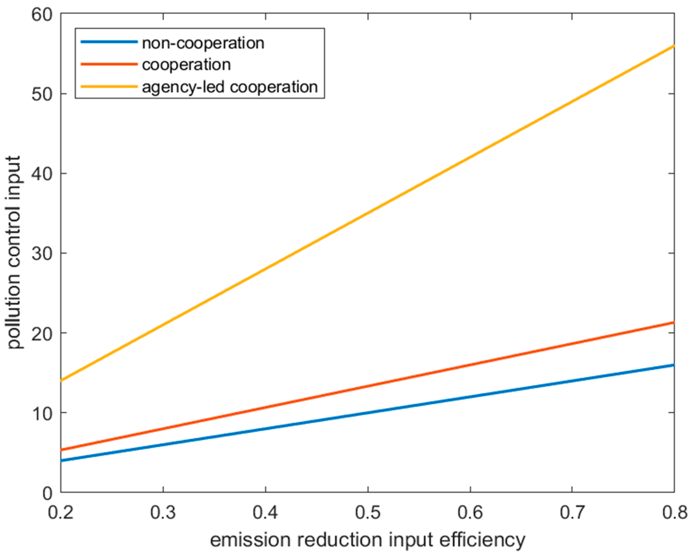
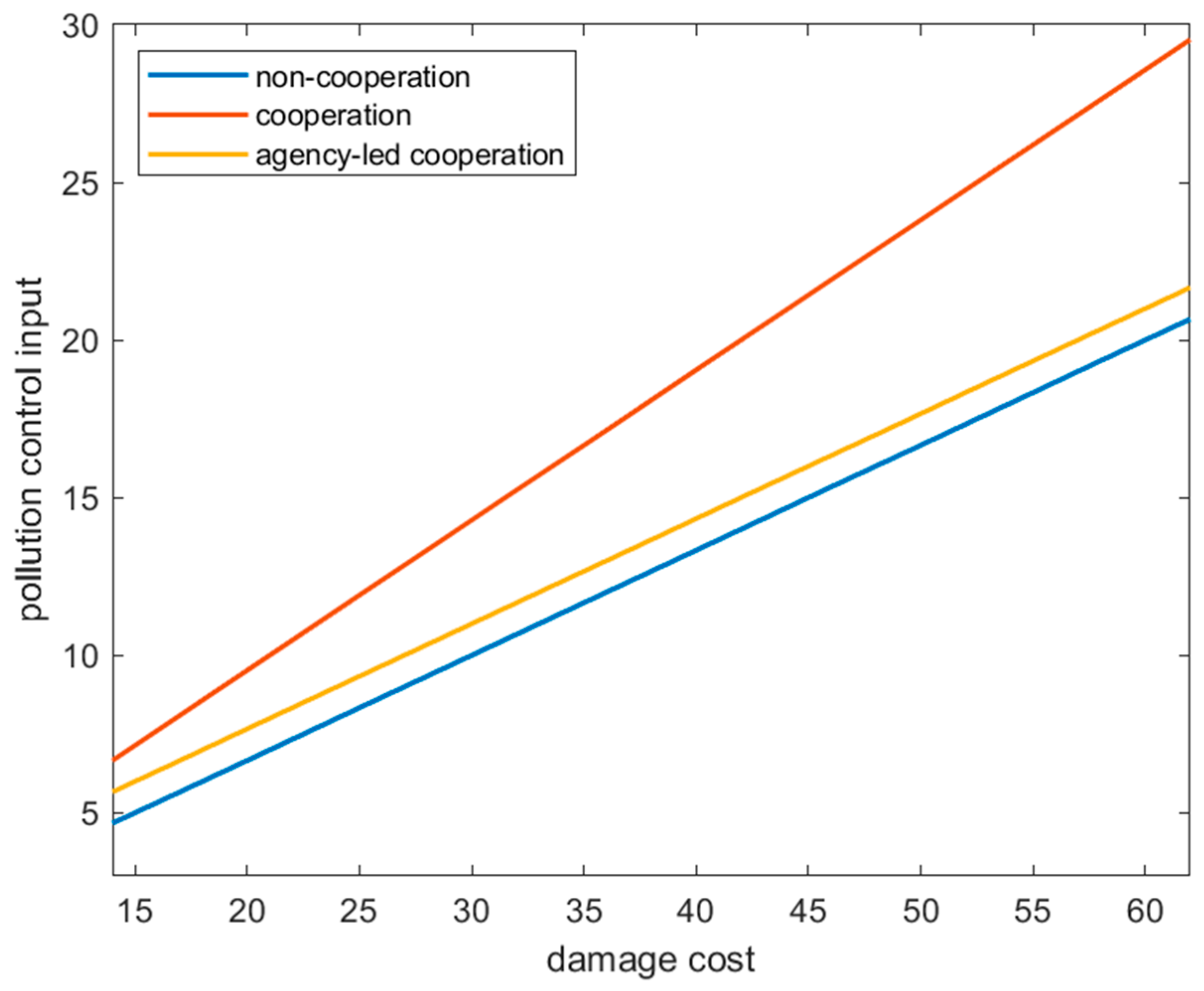
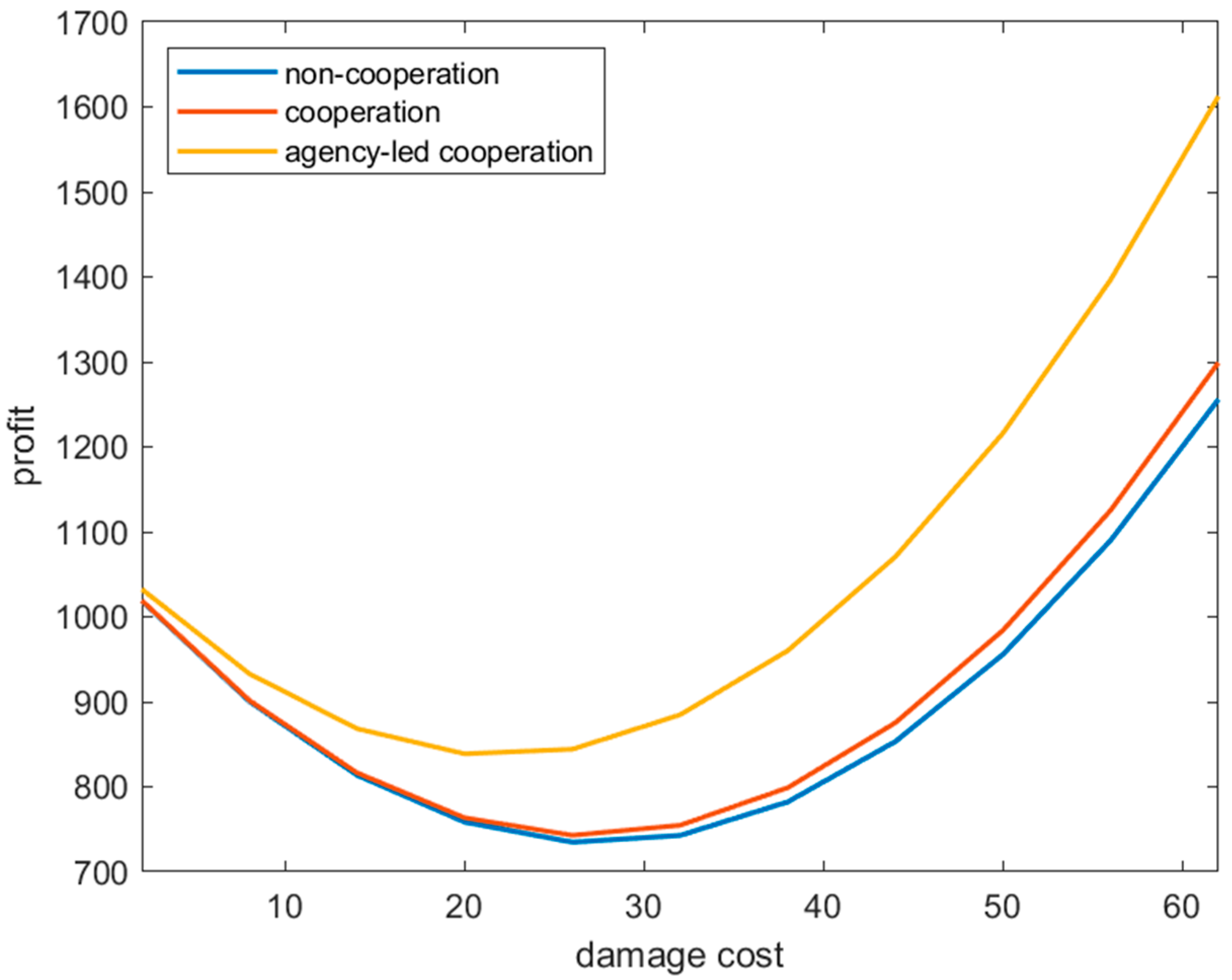
4.2. Simulation Analysis

After analyzing the equilibrium strategies for water pollution control under three scenarios, some conclusions could not be clearly presented due to the complexity of scenarios. This section employs MATLAB software as an analytical tool to verify the calculation results of water pollution in the river basin under different scenarios through practical examples. A sensitivity analysis is conducted on the optimal strategies of local governments and their influencing factors, aiming to gain more insightful understanding. Drawing reference from relevant data in the Three Gorges Reservoir Region of the Yangtze River Basin, where water pollution control is jointly undertaken by the river basin management authority and the upstream and downstream local governments, model parameters are assigned values under this context as follows:

$$b_U=30, b_D=40, {\gamma }_U=0.6, {\gamma }_D=0.4, {\mu }_U={\mu }_D=0.2, d_U=2, d_D=3, \delta =0.1, \alpha =0.25.$$

By substituting each parameter into the analytical equation in the previous section, the decision-making and benefits of the upstream and downstream regional governments can be obtained, as well as the profit situation.

Based on the comparative analysis, as well as the assignment of parameters, the impact of changes in emission reduction input efficiency on pollutant control inputs, as well as profits in the upstream areas under three management scenarios is analyzed, as shown in Figure 1 and Figure 2.

As can be seen in Figure 1 and Figure 2, water pollution control inputs and total basin revenues under the non-cooperation scenario, the cooperation scenario, and the basin agency-led cooperation scenario all rise as emission reduction efficiency increases. The water pollution control inputs and total basin revenues under the cooperation scenario led by the basin agency are the highest, followed by water pollution control inputs and total basin revenues under the cooperation scenario, and the lowest are water pollution control inputs and total basin revenues under the non-cooperation scenario. The results indicate that improving abatement efficiency contributes to increased water pollution control inputs and total basin revenues. In the cooperation scenario led by the basin agency, both water pollution inputs and total basin revenues are at the highest level because the basin agency is able to coordinate the interests of all parties, integrate resources, and promote the joint management of the water pollution problem. In contrast, in the cooperation scenario, although the parties may coordinate their actions, the lack of a central steering body may result in lower water pollution inputs and lower total basin revenues than in the cooperation scenario led by the basin agency. In contrast, in the non-cooperation scenario, parties tend to put their own interests first, resulting in relatively low water pollution control inputs and total basin revenues. These results highlight the importance of basin-level governance mechanisms and suggest that synergies and basin-level governance mechanisms need to be taken into account to achieve optimal levels of water pollution inputs and total basin revenues when managing water pollution problems.

Water pollution discharges not only cause damage to local ecosystems, water resources and environmental quality, but may also affect upstream and downstream areas, leading to economic losses and social problems. Analyzing damage costs can help decision-makers better understand the severity of the water pollution problem and the extent of its impacts, so the impacts of damage costs on water pollution control inputs and total basin revenues are analyzed for the three management scenarios, as shown in Figure 3 and Figure 4.

As can be seen in Figure 3, as damage costs increase, water pollution control inputs increase in the non-cooperation scenario, the cooperation scenario and the basin agency-led cooperation scenario. The highest inputs occur in the cooperation scenario, followed by the basin agency-led cooperation scenario, and lowest in the non-cooperation scenario. The results show that water pollution inputs increased in all scenarios as the cost of damages increased, suggesting that parties are more willing to invest more resources in combating water pollution problems in the face of more severe environmental damages. In the cooperation scenario, the parties work together and integrate resources, so they can achieve more efficient water pollution control inputs and better water pollution control results.

As can be seen in Figure 4, as the cost of damages increases, the overall basin revenue decreases and then increases for the non-cooperation scenario, the cooperation scenario, and the basin agency-led cooperation scenario. Overall basin revenues are the highest in the basin agency-led cooperation scenario, followed by the cooperation scenario, and lowest in the non-cooperation scenario. The results suggest that overall basin revenues may decline first in the face of higher impairment costs, due to the fact that increased costs of water pollution control inputs may have some negative impact on economic activity within the basin. However, to a certain extent, environmental quality may improve as water pollution control inputs increase, thereby increasing the sustainability and effectiveness of economic activities within the basin, which in turn leads to an increase in overall basin benefits. In a cooperation scenario led by the basin agency, the overall basin benefits can be maximized due to organized cooperation and coordination of resources, as all parties are able to address environmental challenges more effectively, achieving optimal governance effects and economic benefits. As the downstream local governments share the upstream local governments’ water pollution control and emission reduction costs under the cooperation scenario, the upstream local governments will be motivated to control water pollution and emission reduction, resulting in the improvement of the basin’s ecological environment.

5. Conclusions and Implications

This paper investigates the collaboration between upstream local governments and downstream local governments in the management of cross-border water pollution, taking into account the cost of water pollution control inputs, the natural attenuation rate of pollutants, the emission reduction input efficiency, and damage costs on regional profits. The equilibrium values of the three strategies are solved by establishing the non-cooperation scenario, the cooperation scenario, and the basin agency-led cooperation, and a comparative analysis is conducted. The results of the study show that the model is stable and reliable, and the conclusions obtained have a certain degree of credibility.

5.1. Conclusions

(1)

The balanced results comparing the three management scenarios indicate that, when the upstream region actually discharges water pollution, the scenario led by the river basin authority results in the lowest upstream emissions, the highest investment in water pollution treatment, and the highest total benefit for both upstream and downstream regions. Therefore, the cooperation strategy under the leadership of the river basin authority is optimal.

(2)

Improving abatement efficiency helps increase water pollution control inputs and total basin revenues. This highlights the importance of basin governance mechanisms and emphasizes the key role of synergies and basin management in addressing water pollution.

(3)

As damage costs increased, water pollution control inputs increased in all scenarios, with the highest total revenues in the basin agency-led cooperation scenario, followed by the cooperation scenario and the lowest in the non-cooperation scenario.

5.2. Implication

(1)

The governments of upstream and downstream regions should actively promote the establishment and development of cross-border cooperation mechanisms to facilitate the coordination and integration of water pollution management inputs. Basin-based cooperation platforms or institutions should be established to promote the joint participation of all parties in water pollution management and the sharing of costs and benefits.

(2)

Through cooperation, all parties can optimize the allocation of resources and improve the efficiency of water pollution control inputs. The government and enterprises should rationalize the allocation of resources according to the actual situation and focus on supporting the research and development and application of water pollution control technologies to improve the effectiveness of water pollution control.

(3)

Recognize the importance of the cost of environmental damage to enterprises and society, and take measures to strengthen environmental monitoring and assessment, establish an environmental protection fund and promote green technological innovation, thereby reducing the social cost of water pollution control and realizing a win-win situation in terms of both economic and social benefits.

The non-cooperation scenario decision-making under the cooperation scenario, as designed in this paper, can lead to the overall gain of the basin, but when there is water pollution discharge upstream, it does not reach the optimal level of gain achieved through the basin agency-led decision-making under the cooperation scenario. Further design of other contractual mechanisms to achieve the ideal situation is the direction of further research in the future.

References

1. Li, M.X.; Zou, S.R.; Jing, P.R. Spatial Spillover Effect of Water Environment Pollution Control in Basins-Based on Environmental Regulations. Water 2023, 15, 3745. [Google Scholar] [CrossRef]
2. Ma, T.; Sun, S.; Fu, G.T.; Hall, J.W.; Ni, Y.; He, L.H.; Yi, J.W.; Zhao, N.; Du, Y.Y.; Pei, T.; et al. Pollution exacerbates China’s water scarcity and its regional inequality. Nat. Commun. 2020, 11, 650. [Google Scholar] [CrossRef]
3. Fletcher, R.; Büscher, B. The PES Conceit: Revisiting the Relationship between Payments for Environmental Services and Neoliberal Conservation. Ecol. Econ. 2017, 132, 224–231. [Google Scholar] [CrossRef]
4. Wine, M.L. Under non-stationarity securitization contributes to uncertainty and Tragedy of the Commons. J. Hydrol. 2019, 568, 716–721. [Google Scholar] [CrossRef]
5. Sigman, H. Transboundary spillovers and decentralization of environmental policies. J. Environ. Econ. Manag. 2005, 50, 82–101. [Google Scholar] [CrossRef]
6. Zeng, Y.; Li, J.B.; Cai, Y.P.; Tan, Q.; Dai, C. A hybrid game theory and mathematical programming model for solving trans-boundary water conflicts. J. Hydrol. 2019, 570, 666–681. [Google Scholar] [CrossRef]
7. Yi, Y.X.; Ding, C.N.; Fu, C.Y.; Li, Y.Q. Transboundary watershed pollution control and product market competition with ecological compensation and emission tax: A dynamic analysis. Environ. Sci. Pollut. Res. 2022, 29, 41037–41052. [Google Scholar] [CrossRef]
8. Huang, X.F.; Hua, W.W.; Dai, X.Y. Performance Evaluation of Watershed Environment Governance—A Case Study of Taihu Basin. Water 2022, 14, 158. [Google Scholar] [CrossRef]
9. Chen, K.; Deng, M.H.; Fan, S.S. Synergetic development assessment of transboundary watershed ecological compensation. Water Sci. Technol. 2023, 88, 1438–1446. [Google Scholar] [CrossRef]
10. Lu, H.W.; Yu, S. Pollutant source analysis and tempo-spatial analysis of pollutant discharge intensity in a transboundary river basin. Environ. Sci. Pollut. Res. 2019, 26, 1336–1354. [Google Scholar] [CrossRef]
11. El Ouardighi, F.; Sim, J.E.; Kim, B. Pollution accumulation and abatement policy in a supply chain. Eur. J. Oper. Res. 2016, 248, 982–996. [Google Scholar] [CrossRef]
12. Guo, G.M.; Duan, R.B. A new method to determine the scale range of environmental damage caused by water pollution accidents. Water Supply 2022, 22, 3968–3979. [Google Scholar] [CrossRef]
13. Jing, S.W.; Liao, L.P.; Du, M.Z.; Shi, E.Y. Assessing the effect of the joint governance of transboundary pollution on water quality: Evidence from China. Front. Environ. Sci. 2022, 10, 989106. [Google Scholar] [CrossRef]
14. Jiang, K.; Merrill, R.; You, D.M.; Pan, P.; Li, Z.D. Optimal control for transboundary pollution under ecological compensation: A stochastic differential game approach. J. Clean. Prod. 2019, 241, 118391. [Google Scholar] [CrossRef]
15. Benchekroun, H.; Martín-Herrán, G. The impact of foresight in a transboundary pollution game. Eur. J. Oper. Res. 2016, 251, 300–309. [Google Scholar] [CrossRef]
16. Bellver-Domingo, A.; Hernández-Sancho, F.; Molinos-Senante, M. A review of Payment for Ecosystem Services for the economic internalization of environmental externalities: A water perspective. Geoforum 2016, 70, 115–118. [Google Scholar] [CrossRef]
17. Jiang, K.; You, D. Study on differential game of transboundary pollution control under regional ecological compensation. China Popul. Resour. Environ. 2019, 29, 135–143. [Google Scholar]
18. Hao, C.L.; Yan, D.H.; Gedefaw, M.; Qin, T.L.; Wang, H.; Yu, Z.L. Accounting of Transboundary Ecocompensation Standards Based on Water Quantity Allocation and Water Quality Control Targets. Water Resour. Manag. 2021, 35, 1731–1756. [Google Scholar] [CrossRef]
19. Li, S.D. A Differential Game of Transboundary Industrial Pollution with Emission Permits Trading. J. Optim. Theory Appl. 2014, 163, 642–659. [Google Scholar] [CrossRef]
20. Li, S.D. Dynamic optimal control of pollution abatement investment under emission permits. Oper. Res. Lett. 2016, 44, 348–353. [Google Scholar] [CrossRef]
21. Huang, X. Transboundary watershed pollution control analysis for pollution abatement and ecological compensation. Environ. Sci. Pollut. Res. 2023, 30, 44025–44042. [Google Scholar] [CrossRef]
22. Chang, S.H.; Qin, W.H.; Wang, X.Y. Dynamic optimal strategies in transboundary pollution game under learning by doing. Phys. A-Stat. Mech. Its Appl. 2018, 490, 139–147. [Google Scholar] [CrossRef]
23. Zhao, L.J.; Qian, Y.; Huang, R.B.; Li, C.M.; Xue, J.; Hu, Y. Model of transfer tax on transboundary water pollution in China’s river basin. Oper. Res. Lett. 2012, 40, 218–222. [Google Scholar] [CrossRef]
24. Song, J.X.; Wu, D.S. An innovative transboundary pollution control model using water credit. Comput. Ind. Eng. 2022, 171, 108235. [Google Scholar] [CrossRef]
25. Sheng, J.C.A.; Webber, M. Incentive coordination for transboundary water pollution control: The case of the middle route of China’s South-North water Transfer Project. J. Hydrol. 2021, 598, 125705. [Google Scholar] [CrossRef]
26. Kolaolusanya, A.; Oyeyemi, E.; Adewale, P.S.; Omobuwa, O. Role of environmental education in water pollution prevention and conservation in Nigeria. Water Supply 2024, 24, 361–370. [Google Scholar] [CrossRef]
27. Jia, F.J.; Wang, D.D.; Zhou, K.; Li, L.S. Differential decision analysis of transboundary pollution considering the participation of the central government. Manag. Decis. Econ. 2022, 43, 1684–1703. [Google Scholar] [CrossRef]
28. Jørgensen, S.; Zaccour, G. Incentive equilibrium strategies and welfare allocation in a dynamic game of pollution control. Automatica 2001, 37, 29–36. [Google Scholar]
29. Cheng, C.G.; Fang, Z.; Zhou, Q.; Wang, Y.D.; Li, N.; Zhou, H.W. Improving the effectiveness of watershed environmental management-dynamic coordination through government pollution control and resident participation. Environ. Sci. Pollut. Res. 2023, 30, 57862–57881. [Google Scholar] [CrossRef]
30. Ma, J.; Cheng, C.G.; Tang, Y. Basin Eco-Compensation Strategy Considering a Cost-Sharing Contract. IEEE Access 2021, 9, 91635–91648. [Google Scholar] [CrossRef]
Figure 1. Impact of emission reduction input efficiency on water pollution control inputs in upstream areas under three management scenarios.
Water 16 02767 g001
Figure 2. Impact of emission reduction input efficiency on the total profits of the three management scenarios.
Water 16 02767 g002
Figure 3. Impact of damage costs on water pollution control inputs of the three management scenarios.
Water 16 02767 g003
Figure 4. Impact of damage costs on total basin profits of the three management scenarios.
Water 16 02767 g004