Abstract
Accurate assessment of water surface velocity (WSV) is essential for flood prevention, disaster mitigation, and erosion control within hydrological monitoring. Existing image-based velocimetry techniques largely depend on correlation principles, requiring users to input and adjust parameters to achieve reliable results, which poses challenges for users lacking relevant expertise. This study presents RivVideoFlow, a user-friendly, rapid, and precise method for WSV. RivVideoFlow combines two-dimensional and three-dimensional orthorectification based on Ground Control Points (GCPs) with a deep learning-based multi-frame optical flow estimation algorithm named VideoFlow, which integrates temporal cues. The orthorectification process employs a homography matrix to convert images from various angles into a top-down view, aligning the image coordinates with actual geographical coordinates. VideoFlow achieves superior accuracy and strong dataset generalization compared to two-frame RAFT models due to its more effective capture of flow velocity continuity over time, leading to enhanced stability in velocity measurements. The algorithm has been validated on a flood simulation experimental platform, in outdoor settings, and with synthetic river videos. Results demonstrate that RivVideoFlow can robustly estimate surface velocity under various camera perspectives, enabling continuous real-time dynamic measurement of the entire flow field. Moreover, RivVideoFlow has demonstrated superior performance in low, medium, and high flow velocity scenarios, especially in high-velocity conditions where it achieves high measurement precision. This method provides a more effective solution for hydrological monitoring.
1. Introduction
Streamflow data constitute a fundamental component of hydrological research and serve as the cornerstone for all hydrological investigations. Particularly amidst the prevalent occurrences of extreme events, such as floods and droughts, the demand for expeditious acquisition of critical information regarding river flow velocity and runoff variations has become increasingly urgent [1]. Traditional velocity measurement methods, such as those utilizing propeller current meters and an Acoustic Doppler Current Profiler (ADCP) [2], although well-established and widely employed for field measurements, are significantly constrained by factors including weather conditions, topography, and hydraulic regimes. Moreover, these methods require manual intervention and are impractical for large-scale deployment. Consequently, they have failed to meet the evolving requirements of modern hydrological measurement practices.
In response to the challenges outlined above and to accomplish remote monitoring tasks, a method for measuring water surface velocity (WSV) based on video imagery has emerged in recent years. This approach has garnered considerable attention due to its notable safety and high measurement efficiency. The fundamental process of this method is as follows: initially, a camera is installed on one side of the riverbank to capture video imagery of the river surface. Subsequently, an image-based velocimetry method is employed to estimate the pixel-level two-dimensional velocity field of the water flow from the video imagery. Following this, an affine transformation is applied to convert the velocity field into real flow velocities.
Image velocimetry can be divided into Particle Image Velocimetry (PIV), Particle Tracking Velocimetry (PTV), Space-Time Image Velocimetry (STIV), and Optical Flow Velocimetry (OFV), according to difference motion vector estimation methods. PIV, particularly the Large-Scale PIV (LSPIV) proposed by Fujita et al. [3], estimates flow velocities by analyzing the motion of tracer particles captured by high-speed cameras. However, the accuracy of LSPIV is significantly influenced by the density and distribution of tracer particles on the water surface [4]. PTV, a Lagrangian perspective-based method, reconstructs the velocity field by tracking the trajectories of individual particles within the field of view [5,6]. Nevertheless, the performance of PTV is affected by environmental conditions such as lighting, wind speed, and shadows, which are often difficult to control in the field. Although researchers have implemented various measures to reduce the interference of these environmental factors, the collected image data may still contain noise that is challenging to completely eliminate [7]. On the other hand, STIV calculates flow velocities by identifying the texture angle produced by the grayscale changes of flow lines, and while it has a distinct advantage in terms of processing speed, it is highly sensitive to noise [8]. OFV methods, based on the brightness constancy assumption, obtain motion vectors by analyzing pixel displacements between consecutive images. Xu et al. [9] proposed a sub-grid scale variational optical flow algorithm that effectively addresses the issue of sub-grid small-scale structural information not captured in traditional grid-scale optical flow estimation. Wang et al. [10] employed a dense inverse search method, combined with a frame difference approach, to propose a fast optical flow-based flow measurement algorithm that has made significant progress in improving measurement stability. Recently, deep learning-based optical flow estimation methods have demonstrated significant performance advantages in WSV measurements. For instance, the RivQNet algorithm proposed by Ansari et al. [11], which is based on the FlowNet 2.0 network structure [12], although superior to traditional optical flow methods in terms of computational results, still has room for improvement in terms of accuracy.
This study introduces a user-friendly river surface velocity measurement algorithm that combines orthorectification and deep learning-based multi-frame optical flow estimation. Firstly, an implicit camera calibration method based on Ground Control Points (GCPs) is proposed, eliminating the need for additional chessboard images to obtain camera parameters. Using the calibration results, only four GCPs are required to perform two-dimensional or three-dimensional orthorectification, transforming the image into a “bird’s eye” view. Subsequently, the VideoFlow [13] multi-frame optical flow network, which fully considers the temporal continuity of flow velocity, is employed to estimate pixel displacement. In contrast to current approaches, this research introduces an innovative method for measuring flow velocity that avoids the need for complex equipment and preliminary processing. This method is particularly valuable for practical applications in monitoring river flow velocities. To verify the feasibility of the proposed method, a multi-scenario river simulation platform was constructed in a laboratory flume with a particular focus on verifying flood-level flow velocity measurements. Experimental results indicate that this method is straightforward to use, highly efficient, and yields reliable outcomes.
2. Materials and Methods
2.1. Image Correction
Due to the large-scale field of view and oblique viewing angles often encountered in river images collected in the wild, it is necessary to use orthorectified images, free from lens distortion and perspective effects, to compute velocity and flow rates. The latter issue makes orthorectification a crucial step. When lens distortion is negligible, the pinhole camera model can be employed. Assuming that the water surface is planar, orthorectification is typically achieved through plane-to-plane projection, matching any real position on the orthorectified plane to the corresponding position on the image plane. This plane-to-plane projection is defined by 11 coefficients, which must be estimated through either implicit or, less commonly, explicit camera calibration. Implicit camera calibration is a standard estimation procedure in which the 11 coefficients are fitted using a limited number of reference points with known images and real-world coordinates [14]. Explicit camera calibration is based on a camera model, with parameters calculated from physical parameters such as camera position and angle, focal length, sensor size, and center location. The 11 coefficients of the plane-to-plane projection can then be derived from the camera model parameters. In this paper, we introduce an implicit camera calibration method and fit the camera extrinsic parameters using GCPs.
2.1.1. Camera Calibration
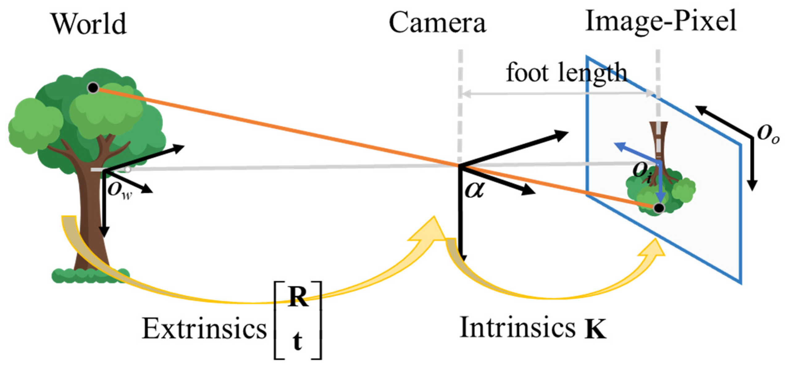
To perform distortion correction and orthorectification of images, both the intrinsic and extrinsic characteristics of the camera are essential. The intrinsic parameters are specific to the camera and include the focal lengths and the principal point coordinates . The extrinsic parameters define the rotation and translation that transforms the world coordinate system into the camera coordinate system. Thus, the extrinsic parameters enable the transformation from the real world to the camera and finally to the image plane, as illustrated in Figure 1. The matrix formula is as follows:
whereas is the camera intrinsic matrix is the rotation matrix, transforming the world coordinate system to the camera coordinate system, and is the translation vector, translating the world coordinate system to the camera coordinate system. s is the scale factor.

Figure 1.
Coordinate transformation using camera intrinsics and extrinsics.
For the estimation of the extrinsic parameters and , the scale factors, we employ GCP fitting. This involves minimizing the projection error of 3D points onto the image plane using the Levenberg-Marquardt [15] non-linear optimization algorithm. The error is defined as the distance between the projected points and the actual 2D image points. Given as the 3D points and as the corresponding 2D points, along with the camera intrinsic matrix and distortion coefficients , we solve for and such that:
The project function maps the 3D point Pi onto the 2D image plane by applying the rotation , translation , distortion correction, and intrinsic projection.
2.1.2. Distortion Correction
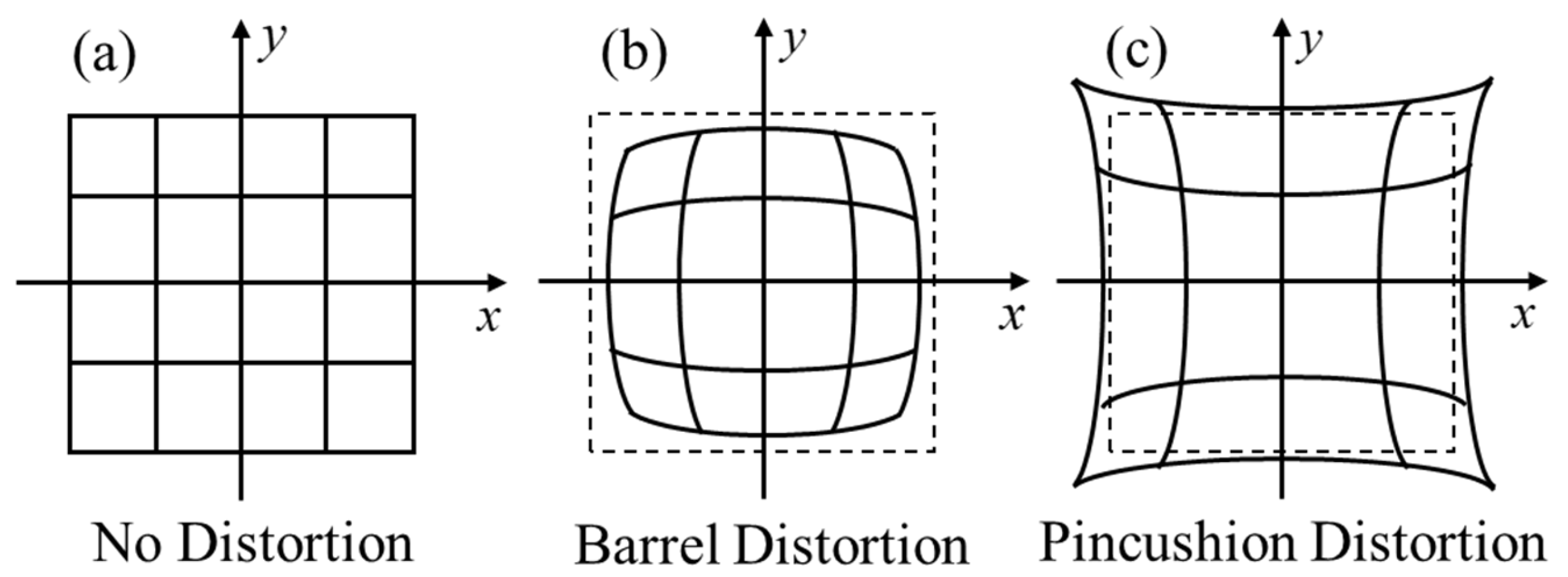
The two main types of distortion are radial and tangential. Radial distortion causes straight lines to appear curved, which is due to the shape of the lens. This effect is more pronounced for points farther from the image center. Two types of radial distortion can occur: a positive one known as Barrel distortion and a negative one known as Pincushion distortion. These are illustrated in Figure 2. When employing image velocimetry to measure WSV, correcting for radial distortion is crucial because the magnitude and direction of the velocity vectors are affected. As the magnitude decreases, vectors farther from the center become smaller (Figure 2b); radial distortion can be corrected using the polynomial in Equation (4).
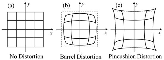
Figure 2.
Types of radial distortion. (a) No distortion; (b) Barrel distortion; (c) Pincushion distortion.
and are the image coordinates after radial correction, while , , and are parameters to be determined, which can be calculated during camera calibration. is the radial distance from the image center to the point, i.e., . In addition, a comprehensive image distortion correction model should also include tangential distortion. The most commonly used method for addressing tangential distortion is the Brown-Conrady model [16].
2.1.3. Orthorectification
Orthorectification is the process of performing geometric correction on an image to eliminate distortions caused by perspective projection, presenting the image from an overhead viewpoint while preserving the relative sizes of the objects within the image. The simplest method for capturing images or videos of a river is to capture images from the shore. However, due to the influence of the camera angle, the velocity vectors obtained from optical flow calculations may exhibit some distortion. To address this, we employ a non-parametric orthorectification approach to correct perspective distortion. Specifically, we utilize the extrinsic parameters obtained from camera calibration, including the rotation matrix and translation vector , along with the origin, orientation defined by rotation matrix , and position defined by translation vector of the overhead viewpoint coordinate system, to compute the homography transformation matrix, as shown in Equation (5). This transformation matrix enables conversion from the camera coordinate system to the world coordinate system, as described in Equation (6).
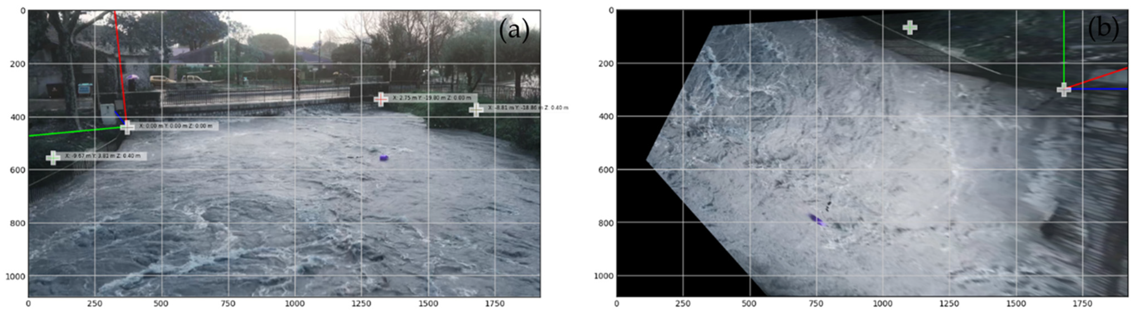
Unlike the RIVeR (2020b) [17] software, which is specialized for the orthorectification of PIV results, our method imposes less stringent requirements on the number and distribution of GCPs. We can perform a two-dimensional transformation using four GCPs located on the same plane as the water surface or a three-dimensional transformation using at least four GCPs not confined to the same plane. In either case, a greater number of GCPs will enhance the accuracy of the transformation. Figure 3 presents the orthorectification results of an image of the Braque River [18] captured from a bridge using four GCPs located on different planes.
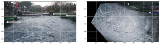
Figure 3.
Orthorectification Impact on Braque River Imagery. (a) A sample frame of the Braque River captured by a camera mounted on a bridge; (b) The orthorectified version of the image in (a). The plus symbols depicted in the image represent the three-dimensional coordinates of the four Ground Control Points (GCPs) within the world coordinate system.
2.2. Principle Analysis of OFV Method
Traditional optical flow. Traditional optical flow estimation is a crucial problem in computer vision, aiming to infer the displacement field of objects between consecutive frames in an image sequence. Traditional methods treat optical flow estimation as an optimization problem, relying heavily on handcrafted features to quantify the similarity between image pairs. While performing well in some scenarios, traditional approaches may struggle with complex image scenes, especially those with discontinuous textures or drastic changes in lighting. Hence, with the advancement of deep learning techniques, recent years have witnessed a gradual shift towards deep learning-based optical flow estimation methods, which have demonstrated superior performance compared to traditional handcrafted feature-based methods.
Deep learning-based two-frame and multi-frame optical flow. In this study, we adopted the VideoFlow optical flow estimation framework, which further develops upon existing two-frame optical flow estimation techniques. Specifically, FlowNet [19], as the first convolutional neural network (CNN)-based end-to-end optical flow network, uses an encoder-decoder structure and a feature pyramid to predict optical flow at different scales. While FlowNet and its derivatives [12,20,21] have made big strides in optical flow estimation, they sometimes struggle with multi-scale flows and subtle motions. This can result in rough predictions, which may cause errors in further calculations. To address this issue, the RAFT [22] model was integrated, which iteratively refines the flow field through correlation volumes and cyclic Conv-GRU units, significantly enhancing the accuracy of optical flow estimation. Furthermore, with the emerging advantage of transformer architectures in capturing fine spatio-temporal details, transformer-based optical flow estimation models, such as GMFlow [23] and FlowFormer [24], have gained attention. These models further improve performance by more effectively modeling spatio-temporal dependencies. The VideoFlow architecture extends the GMFlow two-frame optical flow estimation model by incorporating temporal coherence across consecutive frames, effectively computing bidirectional optical flow within multiple frames. This approach not only improves the accuracy of optical flow estimation but also enhances the model’s adaptability to complex dynamic scenes, which is crucial for flow velocity measurement in hydrology.
2.3. Model Features and Architectures of VideoFlow
VideoFlow is an advanced framework designed to estimate optical flow in video sequences. It effectively calculates bidirectional optical flows across multiple frames by utilizing temporal information. The method involves segmenting the input video into overlapping sets of three frames each. The Tri-frame Optical Flow (TROF) module processes each set individually, while the Motion Propagation (MOP) module integrates these outputs to produce a comprehensive multi-frame optical flow estimation.
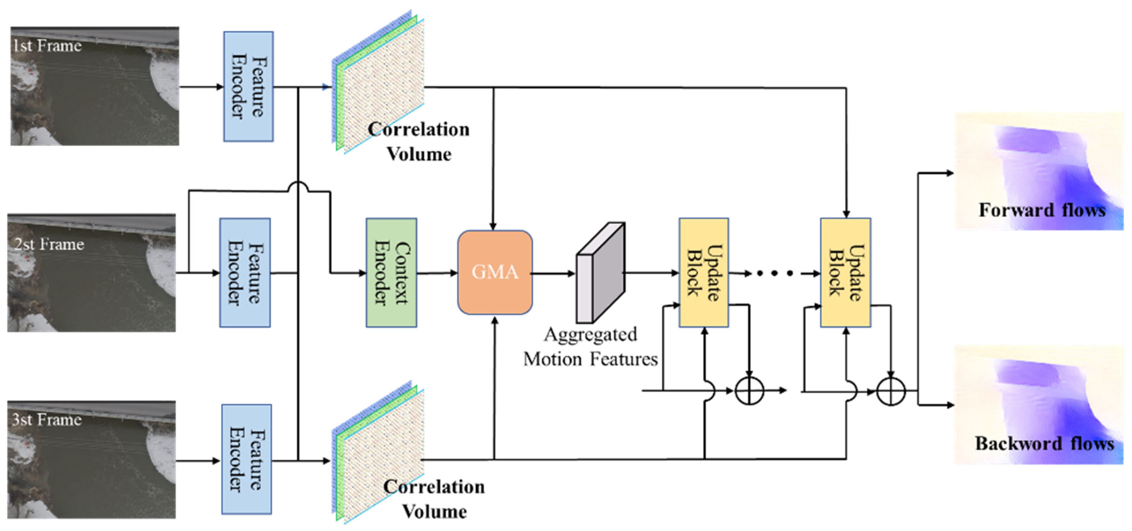
2.3.1. TROF for Tri-Frame Optical Flow Estimation
The TROF module is specifically designed to forecast bidirectional optical flows within sequences of three contiguous frames . It iteratively calculates a series of bidirectional flows , encompassing both forward flows and backward flows , where denotes the iteration step. TROF primarily comprises four stages: extraction of features from three frames via a Twins-SVT [25] encoder, computation of dual all-pairs correlation cost volume, fusion of bidirectional motion features, and iterative updates based on super kernel blocks. It is noteworthy that, apart from employing the Twins-SVT encoder for feature extraction, the rest of the process relies on SKBlock [26] composed of large-kernel deep convolutional layers. The TROF framework is depicted in Figure 4.
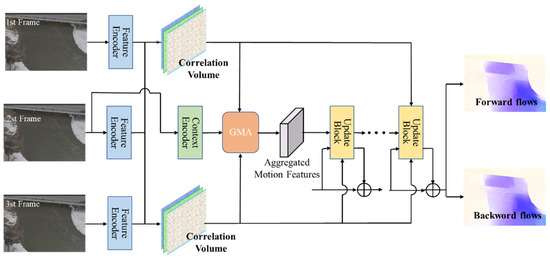
Figure 4.
Tri-frame optical flow framework of VideoFlow.
The process of bi-directional motion feature fusion in TROF. The essence of the TROF method lies in the effective integration of bidirectional motion information into the central frame within the temporal dimension. Following a methodology akin to the RAFT method, TROF initially employs a feature encoder based on Twin-SVT to convert the three input images into feature maps. These feature maps are subsequently utilized to compute bidirectional correlation volumes from the central frame to the previous and next frames i.e., and , quantifying pixel-wise visual similarities between pairs of images. Additionally, it guarantees that both flows emanate from a shared pixel location and form a cohesive trajectory in the temporal domain. TROF iteratively optimizes bidirectional flows by accessing multiscale correlation values associated with the current central flow. Specifically, in each iteration, based on the currently estimated bidirectional flows , , correlation values are retrieved from the dual correlation volumes and amalgamated into the central frame. The fused correlation features and flow features encode dual correlation values and displacements, respectively. These features are then further encoded to derive bidirectional motion features , encapsulating abundant motion and correlation information crucial for predicting the remaining bidirectional flows, as elaborated further below.
Updating of Bi-directional Recurrent Flow. During the bidirectional recurrent update process of TROF, a Super Kernel Block is utilized as the updater instead of Conv-GRU in RAFT. Nonetheless, it still maintains a hidden state or feature caching to refine the flow. Motion features, context features, and hidden state features are passed into the recurrent update module to update the hidden state. Context features are derived from the visual features of the central frame, and bidirectional residual flows are decoded from the hidden state.
The accumulated residual flows refined at each iteration constitute the final predicted optical flow.
2.3.2. Motion Propagation for Multi-Frame
To extend the network architecture to handle more than three frames, a motion propagation module is introduced in the recurrent update decoder. This module facilitates the propagation of bidirectional motion features along the anticipated “flow trajectories”. Specifically, to effectively propagate information between adjacent TROFs, an additional motion state feature is maintained within each TROF unit. By integrating the warped adjacent TROFs’ motion state features and into the current TROF unit, the motion information gradually propagates throughout the entire sequence over multiple iterative cycles.
In each iteration, temporal motion information is extracted from adjacent TROF units and concatenated with the current frame’s motion state feature to form the motion propagation feature . This feature enhances the coherence and flow attributes of the current frame by consolidating the motion features of the adjacent TROF units. Meanwhile, the motion feature state is also updated. Ultimately, through the MOP module, the hidden motion features of adjacent TROF units are gradually assimilated, allowing the temporal perception domain of the hidden motion features to expand with each iteration, thus enabling more effective handling and integration of additional TROF units, and extending the effective temporal span.
2.4. Video Acquisition and Data Processing
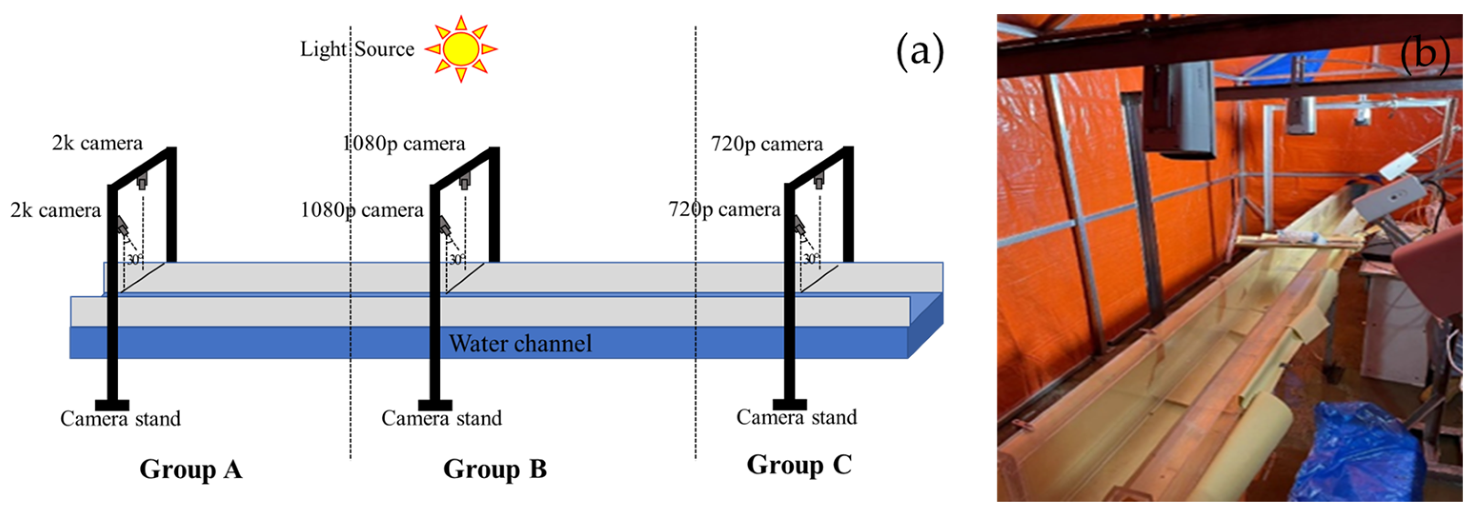
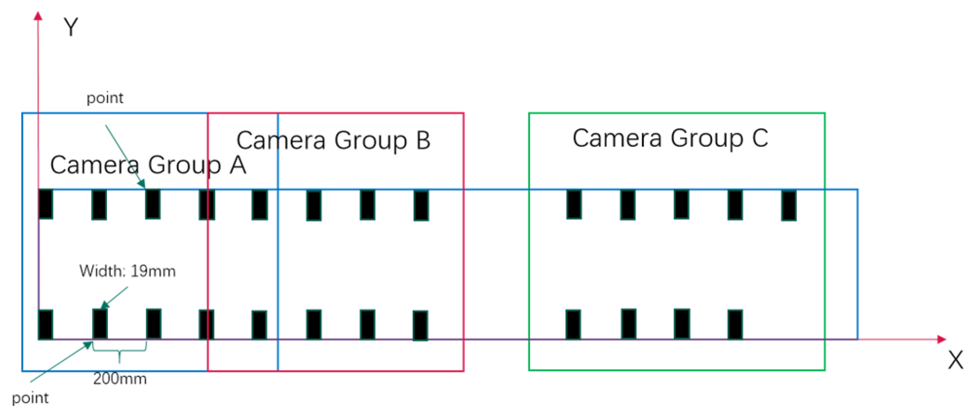
In the laboratory of Hohai University, we have established a multi-camera experimental platform aimed at simulating real river environments and capturing high-quality image data. The platform comprises a flume with dimensions of 4 m in length, 0.177 m in width, and 0.2 m in depth, in addition to six DS-2XA2646F-LZS cameras. These cameras are divided into three groups, each comprising two cameras. One camera in each group captures vertical images to obtain a top-down view of the riverway, while the other camera captures images at a 30-degree angle to acquire a side view of the river surface. The videos captured by each group of cameras have resolutions of 2 k, 1080 p, and 720 p. This layout is designed to acquire image data of multiple angles and resolutions to facilitate a comprehensive analysis of river hydrodynamics. The configuration of the experimental apparatus is depicted in Figure 5. Furthermore, to facilitate camera calibration and conversion of pixel coordinates to world coordinates in image processing, we affixed black tape along the edges of the flume as GCPs, with their layout depicted in Figure 6.
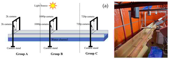
Figure 5.
Experimental setup. (a) Three sets of imaging devices with different resolutions, each consisting of one vertically oriented and one obliquely oriented camera; (b) On-site installation setup of the experimental apparatus.
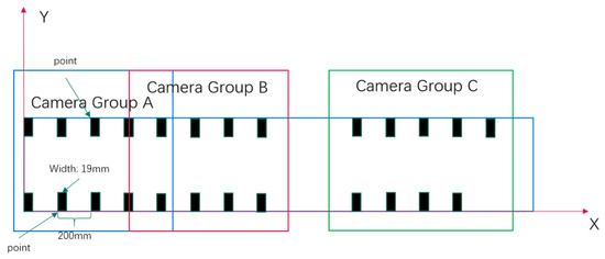
Figure 6.
Distribution of GCPs.
Considering the complexity of real river environments, characterized by varying parameters such as floating debris, water depth, and flow velocity, as well as the influence of different lighting conditions, we have employed multiple strategies to diversify the experimental scenarios. These strategies involve adjusting the density of tracer particles, the water level in the flume, the flow rate at the water interface per unit time, and the position and intensity of illumination sources. Such configurations are intended to provide targeted directions for further algorithm optimization, aiming to adapt to the diverse monitoring tasks of complex river environments in practical applications. The data collection scenarios are detailed in Table 1, with each scenario recorded using six cameras at a frame rate of 25 frames per second for a duration of 120 s. Meanwhile, we conducted instantaneous velocity measurements using a hand-held radar Doppler velocimeter (RDV) at the center and sides of the flume for comparison with image-based velocity estimation methods.

Table 1.
Datasets of various scenarios in the laboratory and their velocity measurement results.
3. Results
3.1. Model Training
In this study, we utilized an NVIDIA RTX 4090 GPU equipped with 24 GB of memory as the hardware platform for our experiments. The experimental environment was constructed based on Python 3.8, CUDA 12.5, and PyTorch 2.0.1. We based our work on previous FlowFormer studies [24], chose the first two stages of the ImageNet pre-trained Twins-SVT [25] model for image and context encoding, and performed parameter fine-tuning on them. Furthermore, following the SKFlow [26], we used SKBlocks instead of ConvGRU to enhance the model’s refinement capabilities.
To bolster the generalization ability of the data, we applied data augmentation techniques such as random cropping, scaling, rotation, and noise addition during the data preprocessing phase. Given the challenges of obtaining comprehensive annotated pixel displacement datasets in real river scenarios and the reliance of the VideoFlow model on dense ground truth, we opted for multiple open-source optical flow datasets to pre-train our model. Specifically, we first conducted pre-training for 125,000 iterations on the FlyingThings [27] dataset, followed by fine-tuning for an additional 25,000 iterations on a combined dataset comprising FlyingThings, Sintel [28], KITTI-2015 [29], and HD1K [30], which is abbreviated as ‘T+S+K+H’. More information about these datasets is provided in Table 2. During the model training process, we employed the AdamW optimizer and implemented a one-cycle learning rate schedule. The batch size was uniformly set to 4 across all training phases. For the FlyingThings dataset, we set the highest learning rate to , while for the other datasets, the highest learning rate was set to . Moreover, the number of updater iterations was established at 16 to ensure that the model learned as much as possible during training.
Table 2.
Details of the FlyingThings, Sintel, KITTI-2015, and HD1K optical flow datasets.
To comprehensively evaluate the effectiveness of our proposed method, we conducted experiments and visual validation using a tank dataset collected in the laboratory, an open-source dataset of the Freiberger Mulde River [31], the Castor River [11], the Hurunui River [32], and the synthetic River datasets created by G. Bodart et al. [33].
3.2. The Simulated River in Laboratory and Analysis of Experimental Results
For a comprehensive evaluation of the method’s robustness in challenging and dynamic scenarios, we applied the RivVideoFlow optical flow estimation algorithm to datasets of 720 p water flow velocity videos collected. The detailed results of velocity estimation are shown in Table 1. Here, RDV-Velocity represents the average velocity collected by RDV in the center of the flume. Mid-Velocity denotes the average velocity estimated by the RivVideoFlow algorithm within the corresponding region of interest (ROI) with values [60:660, 570:620]. Max-Velocity represents the maximum value estimated within the water flow area. According to the results in Table 1, the RivVideoFlow model performs well in river scenes with velocities below 2 m/s, with errors within 15%, even in scenarios where there are no tracers and shadows. However, when the actual velocity exceeds 2.5 m/s, and there are no tracers present on the river surface, the accuracy of velocity estimation decreases significantly. For the experimental groups with tracers, the estimated results are relatively close to the actual values but exhibit instability and a more dispersed velocity distribution. This may be due to foam or splashes formed by internal turbulence at high velocities, causing waves to obscure or reflect camera light, thereby blurring video images and affecting ripple edge detection and contour extraction. When the river velocity exceeds 3.5 m/s, even the estimated pixel-level maximum velocity is lower than the actual velocity, indicating that the proposed model is no longer applicable. A significant observation is that because of the small size of the flume and the camera’s close proximity to the water surface, each pixel in the captured images represents a relatively small actual distance. In other words, the displacement resolution of the images, measured in pixels per meter (ppm), is significantly higher than that of images captured under real river conditions. Typically, the ppm in real river environments is approximately several tens, whereas our laboratory data achieves a ppm of up to 1220. Consequently, the RivVideoFlow method can measure flow velocities much higher than 3.5 m/s in our laboratory setting, indicating its potential to measure even higher velocities in actual river environments. Additionally, we compared our method with the LSPIV velocity estimation method. Figure 7b shows the rendering results of velocity estimation using the well-known Fudda-LSPIV 1.7.3 velocity measurement software for the data highlighted with gray shading in Table 1 [34].
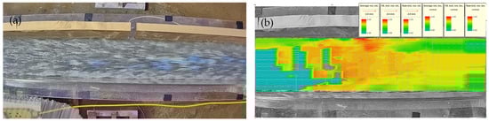
Figure 7.
(a) Aerial view of the water surface in the flume captured by the overhead camera; (b) Surface velocity distribution obtained using the Fudda-LSPIV 1.7.3 software.
3.3. Field River Measurements and Algorithm Validation
3.3.1. The Freiberger Mulde River in Field
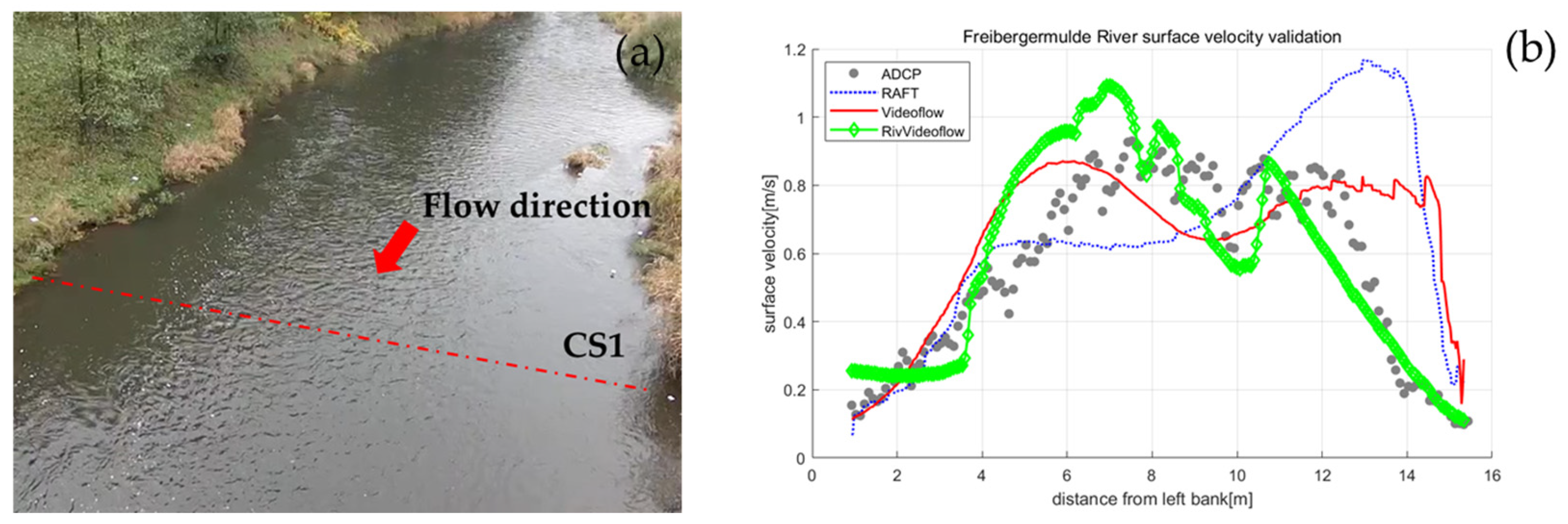
To investigate the application of the RivVideoFlow method for surface velocimetry in natural environments, field measurement data from the Freiberger Mulde River were utilized [31]. These data were captured by a drone hovering over the area of interest at an altitude of 30 m. During data collection, the average water depth was approximately 0.87 m, the average river discharge was 5.60 m3/s, and the average flow velocity was 0.57 m/s. The first 25 s of the recorded video, with a resolution of 640 × 480 pixels and a frame rate of 30 Hz, were used for analysis. Figure 8a displays a sample frame from the recorded video. This serves as an appropriate example for verifying the proposed method’s applicability under low-flow conditions with very clear water. Reference velocity data were collected using an ADCP along the CS1 transect, as shown in Figure 8a.
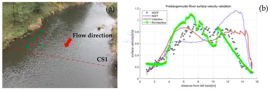
Figure 8.
(a) A sample frame of aerial video of the Freiberger Mulde River showing the ADCP surveyed transect CS1; (b) Surface velocity measurements along CS1 using ADCP and different optical flow methods.
Figure 8b presents the surface velocities measured and estimated at the cross-section CS1 using ADCP and four different optical flow-based surface velocimetry techniques. Figure 9 illustrates the average spatial surface velocity distribution and optical flow fields estimated by the VideoFlow architecture before and after orthorectification. Figure 8b demonstrates that the cross-sectional velocity distribution estimated by the RivVideoFlow method aligns more closely with the reference velocities than in the downstream section. This suggests that the optical flow architecture incorporating temporal cues achieves higher measurement accuracy.
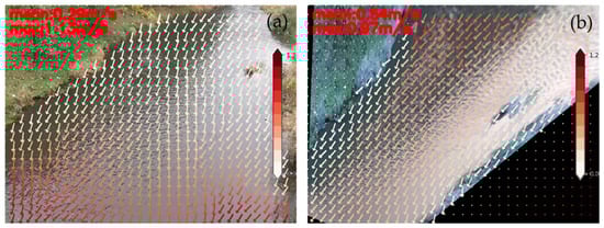
Figure 9.
Averaged surface velocity distribution vector map. (a) The map is estimated using VideoFlow; (b) The map is estimated using RivVideoFlow.
Because of the “near-to-far” effect in the camera’s field of view, one pixel in the upstream section of the Freiberger Mulde River represents a much larger actual distance compared to that in the downstream section. Consequently, the velocity distribution values rendered in the upper part of Figure 9a are relatively low. After orthorectification, the image is transformed from a side view to an overhead view (Figure 9b), resulting in each pixel representing a more consistent actual distance. Therefore, the velocity distribution in Figure 9b appears to be more uniform. In other words, the results depicted in Figure 8 and Figure 9 demonstrate that the RivVideoFlow estimation method, which integrates temporal information and has undergone orthorectification, exhibits superior performance, and produces more accurate and smoother results.
3.3.2. Comparative Analysis of WSV Measurement Techniques
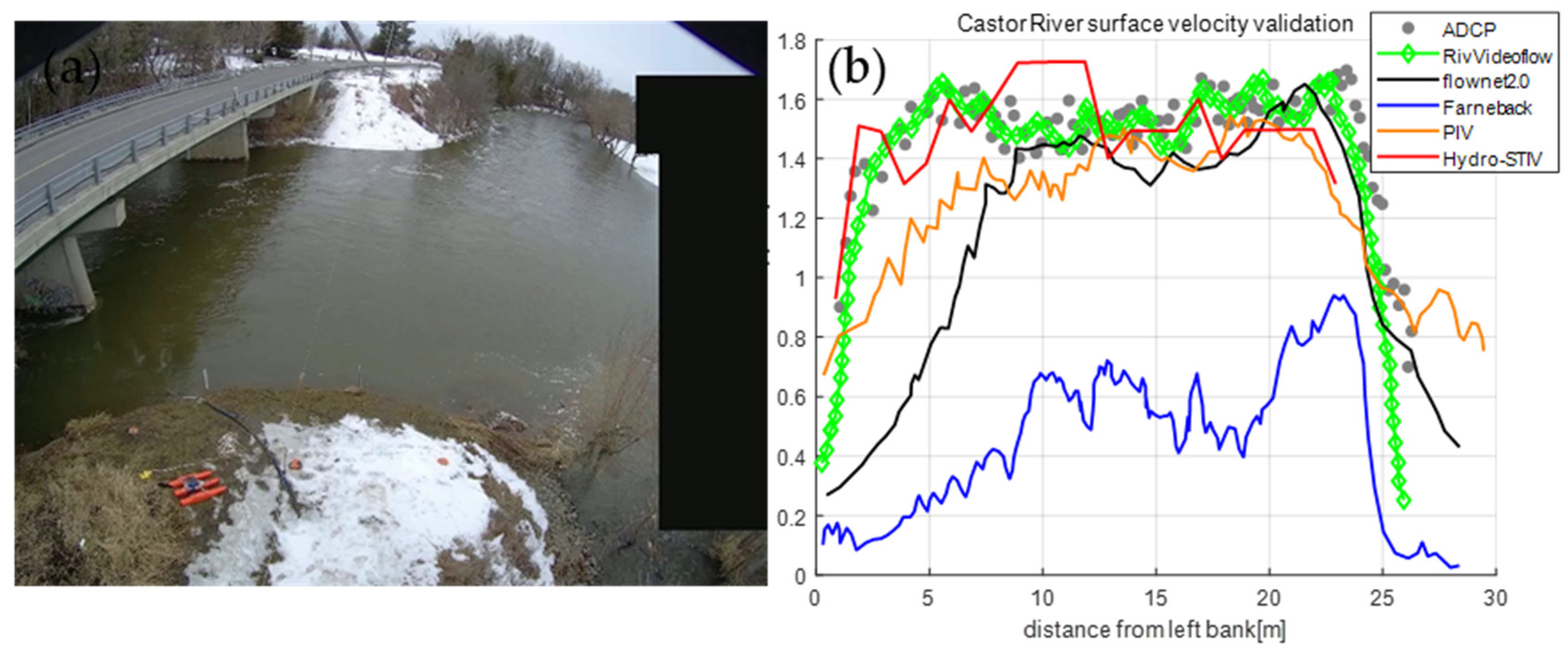
Data acquired from the Castor River on 4 April 2020 [11] underscores the efficacy of diverse image-based methods for assessing WSV. The video dataset, captured at 30 frames per second with a resolution of 2048 × 1536 from a camera positioned on the left bank, spans 29 s and is complemented by concurrent ADCP measurements for precise velocity assessment. On the survey day, the average values for river velocity, discharge, and depth were 1.19 m/s, 13.5 m3/s, and 3.6 m, respectively. The study conditions, marked by optimal diffuse lighting and discernible surface texture across the river’s breadth, presented an ideal scenario for image-based velocity analysis. Spatial calibration was facilitated by documenting twelve ground control points.
The comparative analysis, as depicted in Figure 10, juxtaposes the performance of various image-based velocity measurement techniques with the ADCP data. The traditional Frameback optical flow [35] method was found to be the least accurate, significantly underestimating the river’s surface velocity. Conversely, deep learning-based approaches generally yielded more uniform velocity distributions within the camera’s field of view, outperforming PIV [3] and STIV [36] methods. Notably, the RivVideoFlow technique provided velocity estimates closely aligning with ADCP measurements, highlighting its potential for accurate flow velocity assessment in riverine environments.
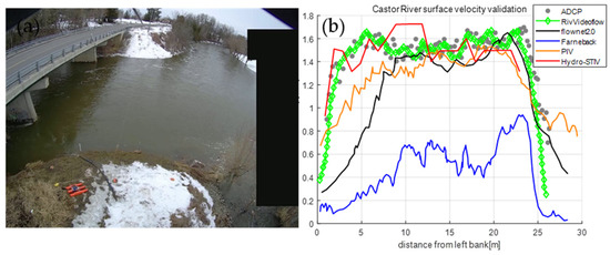
Figure 10.
Comparative Analysis of Cross-sectional Velocity Distributions from Image-Based Flow Velocity Measurement Techniques with ADCP Data at Castor River. (a) Sample frame from the stationary shore-based camera at Castor River. (b) Image-based flow velocity measurements include PIV [3], Hydro-STIV [36], traditional Frameback optical flow method [35], and deep learning network-based optical flow methods such as Flownet2.0 [12] and RivVideoFlow.
3.3.3. Analysis of RivVideoFlow Algorithm Applicable Velocity Range
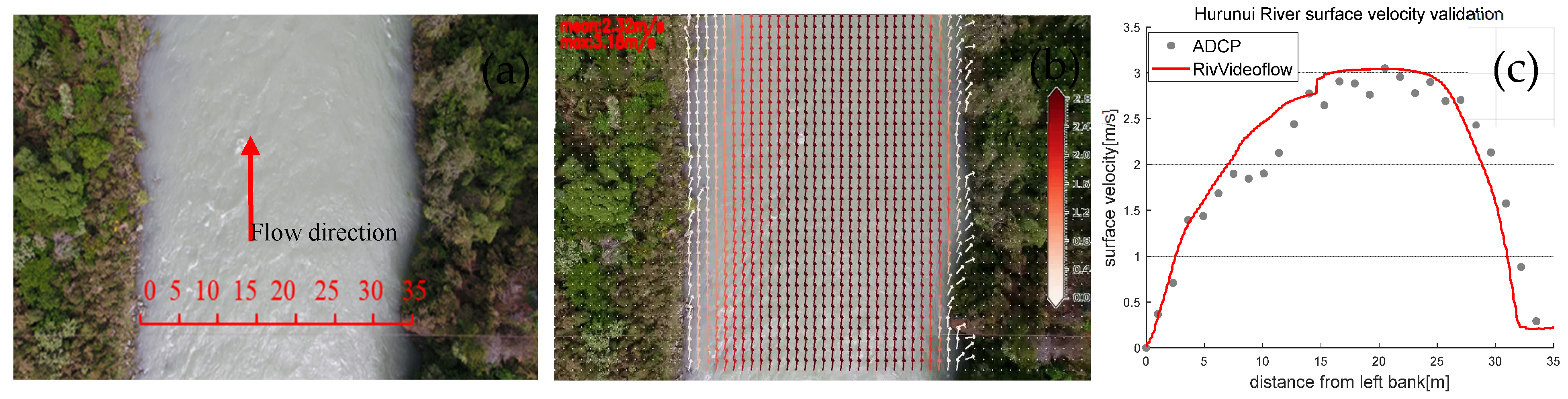
This study utilizes data from the Hurunui River [32] to further assess the RivVideoFlow algorithm’s performance under high-flow conditions. The video dataset of the Hurunui River was captured using a DJI M210 drone and recorded at a frame rate of 24 Hz with a resolution of 3840 × 2160 pixels for a duration of 59 s. Concurrently, actual velocity measurements were obtained through ADCP sampling. Characterized by low water clarity, high flow velocities, a flat riverbed, and a uniformly dense distribution of ripples, the Hurunui River provides a challenging environment for testing the RivVideoFlow algorithm. Analysis, as depicted in Figure 11, indicates that RivVideoFlow performs effectively in measuring high velocities. Moreover, the cross-sectional velocity measurement results presented in Figure 8, Figure 9, Figure 10 and Figure 11 demonstrate that while RivVideoFlow’s performance is somewhat diminished under low-flow conditions in shallow waters, it significantly enhances its performance in high-velocity assessments. Overall, the algorithm shows a relatively strong performance across rivers with varying flow velocities.
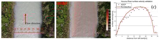
Figure 11.
RivVideoFlow Algorithm Performance under High Flow Conditions in the Hurunui River. (a) A sample frame from the aerial video of the Hurunui River. (b) Averaged surface velocity distribution vector map of the Hurunui River. (c) Surface velocity measurements of the Hurunui River obtained by the RivVideoFlow Algorithm.
3.4. Visualization and Analysis of Experiments on the Synthetic River Datasets
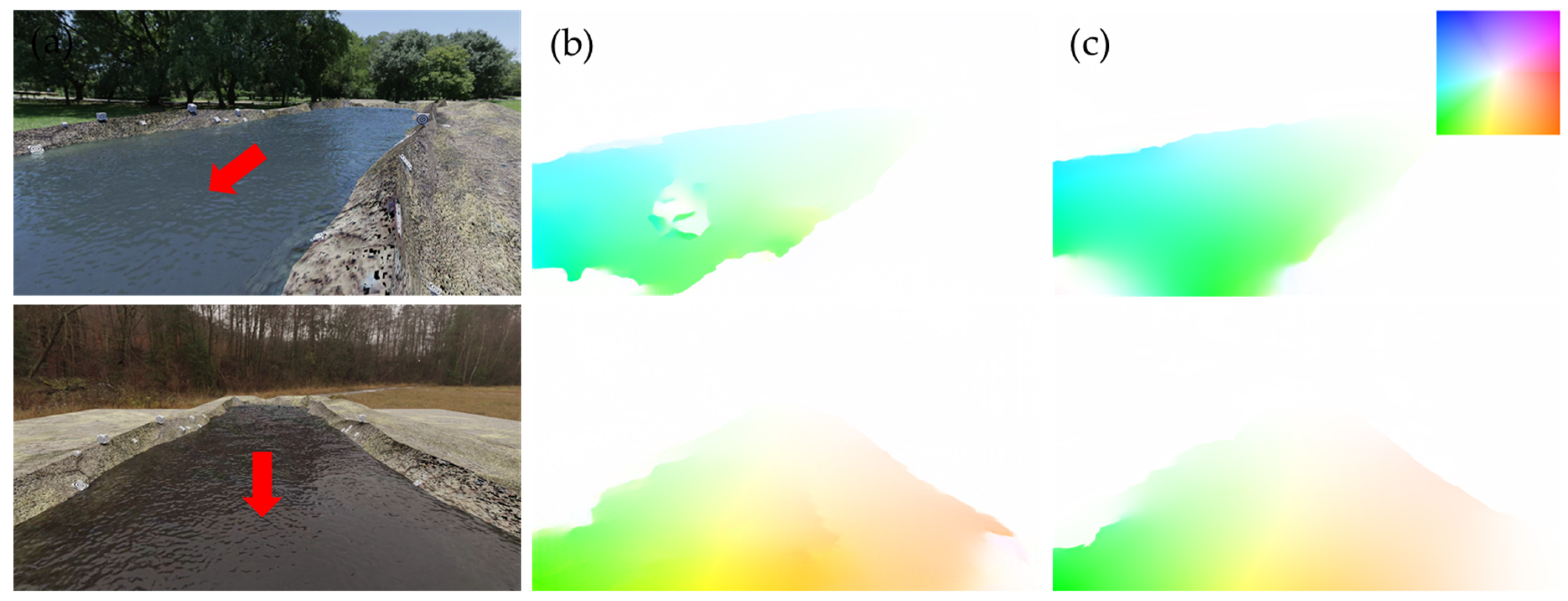
To visually validate the effectiveness and generalization capability of the model, we selected virtual river flow videos from various scenarios, including ideal conditions, sunny weather, cloudy weather, deep forest, and high-altitude drone footage for color-coded visualization of the flow field. Figure 12 illustrates the RSV estimation results for the two scenarios. Scenario one (first row of Figure 12) depicts a sunny day with the river flowing towards the lower left direction, while scenario two (second row of Figure 12) represents a scene captured on the bridge with the river flowing to the right. In scenario one, noticeable cavities are observed in the flow field visualization produced by the RAFT model Figure 12b in the lower left region, mainly attributed to the interference of light and shadows on the river surface in that area, making it challenging for the optical flow-based model to accurately track particle motion. However, in Figure 12c, produced by the RivVideoFlow, no cavities are present, indicating that multi-frame optical flow estimation leveraging temporal cues exhibits better robustness against light and shadow interference.
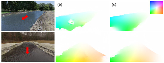
Figure 12.
Visualization of synthetic river flow videos. (a) synthetic river videos; (b) RAFT; (c) RivVideoFlow. The red arrow indicates the direction of river flow. The upper right corner of Figure 12c for Scene 1 is color-coded for the flow field, with the color type indicating the direction of the flow field and the shade indicating flow magnitude.
4. Discussion
This study introduces RivVideoFlow, an innovative video-based technique for quantifying WSV in rivers. This technique employs a homography matrix, denoted as , to orthorectify images, transforming perspectives from oblique angles to a plan-view orientation. This process aligns the visual coordinates of the images with their geographical counterparts in the real world. RivVideoFlow demonstrates high precision and robustness across various datasets, surpassing traditional two-frame RAFT models by effectively integrating temporal information. This integration enhances the method’s capacity to track the continuity of water flow, thereby improving the temporal reliability of WSV measurements.
Despite its reliable estimation of WSV across diverse environmental conditions and its validation against ADCP/RDV measurements, RivVideoFlow has inherent limitations. The performance of RivVideoFlow is reliant on the diversity and representativeness of the training data. The model, which is primarily evaluated under specific conditions, may not adapt seamlessly to the full spectrum of riverine environments. Additionally, while multi-frame optical flow estimation enhances spatiotemporal stability, the algorithm’s precision could be compromised during extreme flow events, such as flash floods or rapids. Furthermore, the presence of substantial river surface debris can degrade the image quality, impacting the accuracy of optical flow estimation. Lastly, RivVideoFlow primarily assesses surface velocities, which may not accurately reflect the average velocity profile across the river, particularly in deeper rivers where surface and sub-surface velocities can significantly differ.
Future research will address three primary objectives. First, we will develop a dataset with dense ground truth annotations for synthetic river videos to enhance model generalizability beyond the current constraints of limited training data diversity. Second, we will refine the optical flow estimation by incorporating physiologically informed constraints within the deep learning model’s loss function, aimed at more accurately capturing fluid dynamics on river surfaces. Lastly, we will investigate methodologies to translate surface velocity measurements into estimates of the average velocity across the river cross-section, which is crucial for a holistic understanding of river flow dynamics.
5. Conclusions
This study successfully developed RivVideoFlow, an innovative video-based method for measuring river surface velocities and monitoring river flow rates. The method integrates lens distortion correction, implicit camera calibration based on Ground Control Points (GCPs), two-dimensional and three-dimensional orthorectification techniques, and a deep learning-based multi-frame optical flow estimation algorithm. The algorithm was tested in various environments, including flood simulation laboratory platforms, outdoor settings, and synthetic river videos. Results indicate that RivVideoFlow can reliably estimate WSV across different flow rates and camera perspectives. Unlike widely used image-based velocity measurement methods such as LSPIV and STIV, RivVideoFlow does not require the deployment of tracers or the adjustment of specific scene parameters. It is a true end-to-end velocity measurement system that operates without manual intervention. We anticipate that RivVideoFlow will facilitate a broader user base, including non-experts, to engage in large-scale image-based velocity measurement applications.
Author Contributions
Conceptualization, G.A., T.D., J.H. and Y.Z.; methodology, G.A. and T.D.; software, G.A. and T.D.; validation, G.A., T.D., J.H. and Y.Z.; resources, G.A. and J.H.; data curation, G.A., T.D. and Y.Z.; writing—original draft preparation, G.A. and T.D.; writing—review and editing, G.A. and J.H.; visualization, T.D.; project administration, Y.Z.; funding acquisition, G.A. All authors have read and agreed to the published version of the manuscript.
Funding
This work was supported by the National Key R&D Program of China (Project Number: 2023YFC3006700; Topic Five Number: 2023YFC3006705).
Data Availability Statement
The data set accessed on 16 July 2024 for the Freiberger Mulde River can be found at https://opara.zih.tu-dresden.de/xmlui/handle/123456789/1405 (accessed on 16 July 2024). The laboratory data presented in this study are available upon request from the corresponding author.
Acknowledgments
Laboratory work was supported by Philippe Gourbesville. We would like to thank the professors in the laboratory of Hohai University for their help with the field campaigns and everyone who helped during the field trials.
Conflicts of Interest
Authors declare that the research was conducted in the absence of any commercial or financial relationships that could be construed as a potential conflict of interest.
References
- Fernández-Nóvoa, D.; González-Cao, J.; García-Feal, O. Enhancing Flood Risk Management: A Comprehensive Review on Flood Early Warning Systems with Emphasis on Numerical Modeling. Water 2024, 16, 1408. [Google Scholar] [CrossRef]
- Laible, J.; Dramais, G.; Le Coz, J.; Calmel, B.; Camenen, B.; Topping, D.J.; Santini, W.; Pierrefeu, G.; Lauters, F. River suspended-sand flux computation with uncertainty estimation, using water samples and high-resolution ADCP measurements. EGUsphere 2024, 2024, 1–32. [Google Scholar]
- Fujita, I.; Muste, M.; Kruger, A. Large-scale particle image velocimetry for flow analysis in hydraulic engineering applications. J. Hydraul. Res. 1998, 36, 397–414. [Google Scholar] [CrossRef]
- Lemos, B.L.H.D.; de Lima Amaral, R.; Bortolin, V.A.A.; Lemos, M.L.H.D.; de Moura, H.L.; de Castro, M.S.; de Castilho, G.J.; Meneghini, J.R. Dynamic mask generation based on peak to correlation energy ratio for light reflection and shadow in PIV images. Measurement 2024, 229, 114352. [Google Scholar] [CrossRef]
- Tauro, F.; Piscopia, R.; Grimaldi, S. Streamflow observations from cameras: Large-scale particle image velocimetry or particle tracking velocimetry? Water Resour. Res. 2017, 53, 10374–10394. [Google Scholar] [CrossRef]
- Gu, M.; Li, J.; Hossain, M.M.; Xu, C. High-resolution microscale velocity field measurement using light field particle image-tracking velocimetry. Phys. Fluids 2023, 35, 112006. [Google Scholar] [CrossRef]
- Tauro, F.; Noto, S.; Botter, G.; Grimaldi, S. Assessing the optimal stage-cam target for continuous water level monitoring in ephemeral streams: Experimental evidence. Remote Sens. 2022, 14, 6064. [Google Scholar] [CrossRef]
- Fujita, I.; Shibano, T.; Tani, K. Application of masked two-dimensional Fourier spectra for improving the accuracy of STIV-based river surface flow velocity measurements. Meas. Sci. Technol. 2020, 31, 094015. [Google Scholar] [CrossRef]
- Xu, H.; Wang, J.; Zhang, Y.; Zhang, G.; Xiong, Z. Subgrid variational optimized optical flow estimation algorithm for Image Velocimetry. Sensors. 2022, 23, 437. [Google Scholar] [CrossRef] [PubMed]
- Wang, J.; Zhu, R.; Zhang, G.; He, X.; Cai, R. Image flow measurement based on the combination of frame difference and fast and dense optical flow. Adv. Eng. Sci. 2022, 54, 195–207. [Google Scholar]
- Ansari, S.; Rennie, C.D.; Jamieson, E.C.; Seidou, O.; Clark, S.P. RivQNet: Deep learning based river discharge estimation using close-range water surface imagery. Water Resour. Res. 2023, 59, e2021WR031841. [Google Scholar] [CrossRef]
- Ilg, E.; Mayer, N.; Saikia, T.; Keuper, M.; Dosovitskiy, A.; Brox, T. Flownet 2.0: Evolution of optical flow estimation with deep networks. In Proceedings of the IEEE Conference on Computer Vision and Pattern Recognition, Honolulu, HI, USA, 21–26 July 2017; pp. 2462–2470. [Google Scholar]
- Shi, X.; Huang, Z.; Bian, W.; Li, D.; Zhang, M.; Cheung, K.C.; See, S.; Qin, H.; Dai, J.; Li, H. Videoflow: Exploiting temporal cues for multi-frame optical flow estimation. In Proceedings of the IEEE/CVF International Conference on Computer Vision, Paris, France, 1–6 October 2023. [Google Scholar]
- Le Coz, J.; Renard, B.; Vansuyt, V.; Jodeau, M.; Hauet, A. Estimating the uncertainty of video-based flow velocity and discharge measurements due to the conversion of field to image coordinates. Hydrol. Process. 2021, 35, e14169. [Google Scholar] [CrossRef]
- Gavin, H.P. The Levenberg-Marquardt Algorithm for Nonlinear Least Squares Curve-Fitting Problems; Department of Civil and Environmental Engineering Duke University: Durham, NC, USA, 2019; Volume 3. [Google Scholar]
- Wang, J.; Shi, F.; Zhang, J.; Liu, Y. A new calibration model of camera lens distortion. Pattern Recognit. 2008, 41, 607–615. [Google Scholar] [CrossRef]
- Patalano, A.; García, C.M.; Rodríguez, A. Rectification of image velocity results (river): A simple and user-friendly toolbox for large scale water surface particle image velocimetry (PIV) and particle tracking velocimetry (PTV). Comput. Geosci. 2017, 109, 323–330. [Google Scholar] [CrossRef]
- Vigoureux, S.; Liebard, L.L.; Chonoski, A.; Robert, E.; Torchet, L.; Poveda, V.; Leclerc, F.; Billant, J.; Dumasdelage, R.; Rousseau, G.; et al. Comparison of streamflow estimated by image analysis (LSPIV) and by hydrologic and hydraulic modelling on the French Riviera during November 2019 flood. In Advances in Hydroinformatics: Models for Complex and Global Water Issues—Practices and Expectations; Springer Nature: Singapore, 2022; pp. 255–273. [Google Scholar]
- Dosovitskiy, A.; Fischer, P.; Ilg, E.; Hausser, P.; Hazirbas, C.; Golkov, V.; Van Der Smagt, P.; Cremers, D.; Brox, T. FlowNet: Learning optical flow with convolutional networks. In Proceedings of the IEEE International Conference on Computer Vision, Santiago, Chile, 7–13 December 2015; IEEE Press: Piscataway, NJ, USA, 2015; pp. 2758–2766. [Google Scholar]
- Sun, D.; Yang, X.; Liu, M.-Y.; Kautz, J. Pwc-net: Cnns for optical flow using pyramid, warping, and cost volume. In Proceedings of the IEEE Conference on Computer Vision and Pattern Recognition, Salt Lake City, UT, USA, 18–22 June 2018; Volume 2, pp. 8934–8943. [Google Scholar]
- Hui, T.W.; Tang, X.; Loy, C.C. Liteflownet: A lightweight convolutional neural network for optical flow estimation. In Proceedings of the IEEE Conference on Computer Vision and Pattern Recognition, Salt Lake City, UT, USA, 18–22 June 2018; pp. 8981–8989. [Google Scholar]
- Teed, Z.; Deng, J. RAFT: Recurrent all-Pairs field transforms for optical flow. In Proceedings of the European Conference on Computer Vision, Glasgow, UK, 23–28 August 2020; Volume 16, pp. 402–419. [Google Scholar]
- Xu, H.; Zhang, J.; Cai, J.; Rezatofighi, H.; Tao, D. Gmflow: Learning optical flow via global matching. In Proceedings of the IEEE/CVF Conference on Computer Vision and Pattern Recognition, New Orleans, LA, USA, 18–24 June 2022; pp. 8121–8130. [Google Scholar]
- Huang, Z.; Shi, X.; Zhang, C.; Wang, Q.; Cheung, K.C.; Qin, H.; Dai, J.; Li, H. Flowformer: A transformer architecture for optical flow. In European Conference on Computer Vision; Springer Nature: Cham, Switzerland, 2022; pp. 668–685. [Google Scholar]
- Chu, X.; Tian, Z.; Wang, Y.; Zhang, B.; Ren, H.; Wei, X.; Xia, H.; Shen, C. Twins: Revisiting spatial attention design in vision transformers. arXiv 2021, arXiv:2104.13840. [Google Scholar]
- Sun, S.; Chen, Y.; Zhu, Y.; Guo, G.; Li, G. Skflow: Learning optical flow with super kernels. Adv. Neural Inf. Process. Syst. 2022, 35, 11313–11326. [Google Scholar]
- Mayer, N.; Ilg, E.; Hausser, P.; Fischer, P.; Cremers, D.; Dosovitskiy, A.; Brox, T. A large dataset to train convolutional networks for disparity, optical flow, and scene flow estimation. In Proceedings of the IEEE Conference on Computer Vision and Pattern Recognition, Las Vegas, NV, USA, 27–30 June 2016; pp. 4040–4048. [Google Scholar]
- Butler, D.J.; Wulff, J.; Stanley, G.B.; Black, M.J. A naturalistic open source movie for optical flow evaluation. In European Conference on Computer Vision; Springer: Cham, Switzerland, 2012; pp. 611–625. [Google Scholar]
- Geiger, A.; Lenz, P.; Stiller, C.; Urtasun, R. Vision meets robotics: The kitti dataset. Int. J. Robot. Res. 2013, 32, 1231–1237. [Google Scholar] [CrossRef]
- Kondermann, D.; Nair, R.; Honauer, K.; Krispin, K.; Andrulis, J.; Brock, A.; Gussefeld, B.; Rahimimoghaddam, M.; Hofmann, S.; Brenner, C.; et al. The hci benchmark suite: Stereo and flow ground truth with uncertainties for urban autonomous driving. In Proceedings of the IEEE Conference on Computer Vision and Pattern Recognition Workshops, Las Vegas, NV, USA, 27–30 June 2016; pp. 19–28. [Google Scholar]
- Bahmanpouri, F.; Eltner, A.; Barbetta, S.; Bertalan, L.; Moramarco, T. Estimating the average river cross-section velocity by observing only one surface velocity value and calibrating the entropic parameter. Water Resour. Res. 2022, 58, e2021WR031821. [Google Scholar] [CrossRef]
- Biggs, H. Drone Flow User Guide v1. 1-River Remote Sensing and Surface Velocimetry; National Institute of Water and Atmospheric Research (NIWA) Report; National Institute of Water and Atmospheric Research (NIWA): Auckland, New Zealand, 2022. [Google Scholar]
- Bodart, G.; Le Coz, J.; Jodeau, M.; Hauet, A. Synthetic river flow videos for evaluating image-based velocimetry methods. Water Resour. Res. 2022, 58, e2022WR032251. [Google Scholar] [CrossRef]
- Le Coz, J.; Jodeau, M.; Hauet, A.; Marchand, B.; Le Boursicaud, R. Image-based velocity and discharge measurements in field and laboratory river engineering studies using the free FUDAA-LSPIV software. In River Flow; CRC Press: Lausanne, Switzerland, 2014; Volume 2014, pp. 1961–1967. [Google Scholar]
- Farnebäck, G. Two-frame motion estimation based on polynomial expansion. In Image Analysis: 13th Scandinavian Conference, SCIA 2003 Halmstad, Sweden, June 29–July 2, 2003 Proceedings 13; Springer: Berlin/Heidelberg, Germany, 2003; pp. 363–370. [Google Scholar]
- Fujita, I.; Watanabe, H.; Tsubaki, R. Development of a non-intrusive and efficient flow monitoring technique: The space-time image velocimetry (STIV). Int. J. River Basin Manag. 2007, 5, 105–114. [Google Scholar] [CrossRef]


Disclaimer/Publisher’s Note: The statements, opinions and data contained in all publications are solely those of the individual author(s) and contributor(s) and not of MDPI and/or the editor(s). MDPI and/or the editor(s) disclaim responsibility for any injury to people or property resulting from any ideas, methods, instructions or products referred to in the content. |
© 2024 by the authors. Licensee MDPI, Basel, Switzerland. This article is an open access article distributed under the terms and conditions of the Creative Commons Attribution (CC BY) license (https://creativecommons.org/licenses/by/4.0/).