Performance of Ergun’s Equation in Simulations of Heterogeneous Porous Medium Flow with Smoothed-Particle Hydrodynamics

Abstract

The flow of water through a channel with a heterogeneous porous layer in its central core is simulated using the method of Smoothed-Particle Hydrodynamics (SPH). Three different porous substrates are considered that differ in the geometry of their grain arrays. The heterogeneity is modeled by dividing the porous substrate into four zones that each have a different porosity. The pressure loss and the flow across the channel are simulated at two different scales, the pore scale and the Representative Elementary Volume (REV) scale, based on use of the Ergun equation. Since the computational cost at the REV scale is much lower than at the pore scale, it is therefore important to assess how accurately the REV-scale calculation reproduces the pore-scale results. The REV-scale simulation predicts cross-sectional mainstream velocity profiles and head losses through the channel that differ from the pore-scale results by root-mean-square errors of about 0.01% and 0.3%, respectively.

1. Introduction

Heterogeneous porous media are characterized by significant variations in porosity and permeability in their structure. They represent a common scenario in numerous natural and artificial systems. From underground aquifers to oil reservoirs, the presence of heterogeneities in the porous structure has an important effect on the fluid flow and related transport processes [1]. Understanding the processes governing this phenomenon is crucial for optimizing production, designing efficient filtration systems, and predicting the behavior of geophysical systems. In particular, the presence of heterogeneities in porous media has significant implications in many applications. For example, in the oil industry, the existence of layers with different porosities and permeabilities significantly affects the efficiency of hydrocarbon extraction and, therefore, the fluid flow distribution and oil recovery [2]. On the other hand, in the management of underground aquifers, heterogeneities can influence water distribution and quality, as well as the migration of contaminants [3].

The study of fluid flow in heterogeneous porous media is an important research area in engineering and geophysical sciences. Since these media exhibit spatial variability in their physical properties, such as porosity, permeability, and pore distribution, the flow behavior is generally highly complex and nonlinear. In the simplest cases where only one physical property varies from one point to another, the degree of apparent heterogeneity depends on three different factors, namely the nature of property variation (frequency distribution), its arrangement (spatial distribution), and the inherent stability of the mechanism being studied [1]. Heterogeneity can arise from various sources, such as variability in material composition, sedimentary deposition, differential compaction, and diagenesis processes. For example, the presence of permeability variations within reservoirs has always been recognized, although their magnitude and relevance have been the subject of debates [1]. Variations in vertical permeability have traditionally been accepted because they can be explained by the nature of deposition processes. However, lateral variations have mostly been overlooked, even though sedimentation is non-uniform over considerable distances within most reservoirs.

Today, numerical methods represent a fundamental tool for the simulation of fluid flow in porous media. However, simulating flow in heterogeneous media represents a unique challenge due to the need to accurately capture the distribution and correlation of heterogeneity across the domain of interest [4]. Due to the intricate porous structure, the interaction between the fluid and the solid matrix is highly complex. In order to address this complexity, two approaches have been employed, namely the pore scale and the Representative Elementary Volume (REV) scale.

The pore scale deals with a detailed description of the fluid–matrix interactions in the micro-structure of the porous medium. Although this approach provides a deep understanding of the underlying physical processes, it is computationally expensive and limited in terms of representativeness at larger scales. In an attempt to address these limitations, models using Machine Learning (ML) have been developed to predict the permeability based on the porosity distribution and other parameters of the porous medium, using techniques such as neural networks, deep learning, and regression methods [4]. In particular, Kamrava et al. [5] proposed an ML approach that incorporates fluid dynamic equations in the learning process. In spite of the fact that their algorithm was trained using a limited dataset corresponding to solutions of the equations over a specific time interval, their approach was seen to yield accurate predictions. Moreover, Ko et al. [4] reported an ML approach that produces an accurate pore-scale description of the flow through synthetic and real reticulated foams.

In contrast, knowledge of the porous medium structure is not required in REV-scale calculations since it is accounted for by simply adding a resistance source term into the momentum equation [6,7,8,9]. A REV is employed to represent the porous matrix, within which the macroscopic properties and flow behavior are assumed to be homogeneous and statistically representative of the medium as a whole [8]. This procedure allows simulations to be carried out on larger scales with a much lower computational cost. In this approach, the Ergun equation is used to calculate the pressure losses caused by viscous dissipation and kinetic energy losses [10]. Ergun’s equation has been used to assess the accuracy of the REV-scale approach in homogeneous porous media [11,12]. It has been also modified to predict pressure losses in randomly packed trickle bed reactors filled with trilobular particles [13]. In addition, Lai et al. [12] proposed a resistance correction coefficient, which takes values between 0 and 1, to improve flow predictions in cases where the structured porous medium of open cells exhibits high porosity. However, there is little work in the literature dealing with applications of the REV-scale approach to the description of fluid flow through heterogeneous porous media. For example, Li et al. [14], with the purpose of understanding packed beds composed of heterogeneous granularity in alternate layers (HAL), developed a coupled LES-LBM-IMB-DEM model to evaluate the interface characteristics of a fluid–solid system, velocity and pore distribution, resistance loss mechanism at the interface, and specific pressure drop relationship between the interface region and the bulk layer section. Also, Li et al. [15] studied the effects of different packing configurations on permeability using CFD tools coupled with the discrete element method (CFD-DEM). In a recent paper, Turkyilmazoglu and Siddiqui [16] studied, by means of a linear stability analysis, how the natural convection inside an impermeable porous channel with imposed isoflux boundary conditions is influenced by the Brinkman–Darcy–Bénard convection model.

In this paper, we investigate the flow of water through a heterogeneous porous layer using Smoothed-Particle Hydrodynamics (SPH) methods. Although microscopic fluid flow characteristics are accurately described at the pore scale, it involves not only a higher computational cost but also inherent difficulty in modeling large-scale systems, since their detailed porous structure is usually not known. Therefore, it is necessary to explore how well the REV-scale approach can reproduce the results at the pore scale with comparable accuracy in the case of water flow through a heterogeneous porous matrix. Most SPH applications to the study of porous media flows are based on the pore-scale approach. For example, Jiang et al. [17] employed SPH techniques to simulate fluid flow in isotropic porous media. In their case, the porous structure was modeled at a mesoscopic level. On the other hand, Tartakovsky et al. [18] studied the effects of pore-scale heterogeneity and anisotropy on flow by means of SPH simulations. Multiphase flows in porous media have also been modeled at the pore scale using SPH methods [19,20,21]. Moreover, SPH models of fluid flow through deformable porous media have also been reported in the literature [22,23]. In these latter simulations, the deformable porous matrix was modeled as an elasto-plastic material and the fluid as incompressible. SPH flow simulations through fractured porous media were also recently reported by Shigorina et al. [24] and Bui and Nguyen [25].

The performance of REV-scale simulations is measured by direct comparison with the results obtained for identical models at the pore scale, using as a benchmark test the flow through a rectangular channel with a heterogeneous porous layer at its center [12]. It is found that the flow dynamics at the REV scale reproduces the pore-scale predictions with fairly good accuracy. The structure of this paper is as follows. Section 2 describes the governing equations and provides details of the numerical methods, while the test model and boundary conditions are given in Section 3. The validation and convergence tests are described in Section 4. The results are discussed in Section 5, and the relevant conclusions are given in Section 6.

2. Basic Equations and SPH Solver

2.1. Governing Fluid Flow Equations

In the absence of thermal effects, the laminar flow of water through a porous layer at the REV scale is completely described by the laws of mass and momentum conservation [26,27],

$${\displaystyle \frac{\partial \rho }{\partial t}}+\nabla ·\left(\rho \mathbf{v}\right)=0,$$

(1)

and

$${\displaystyle \frac{\partial \left(\rho \mathbf{v}\right)}{\partial t}}+\nabla ·\left({\displaystyle \frac{\rho \mathbf{v}\mathbf{v}}{\varphi }}\right)=-\nabla p+\nabla ·\left[\rho \nu \left(\nabla \mathbf{v}+\nabla {\mathbf{v}}^t\right)\right]+\mathbf{F},$$

(2)

respectively. Here $\rho$ denotes the fluid density; $\mathbf{v}$ the fluid velocity vector; p the pressure; $\nu$ the kinematic viscosity; $\varphi$ the porosity of the medium, defined as the ratio between the void volume and the total volume of the porous matrix; and $\mathbf{F}$ the Ergun resistance force to be described in Section 2.2. The superscript t on the right-hand side of Equation (2) means transposition.

Under the assumption that $\nabla \varphi =0$, the above equations can be written in Lagrangian coordinates for smoothed-particle discretization as

$$\begin{array}{ccc}\hfill {\displaystyle \frac{d\rho }{dt}}& =& -\rho \nabla ·\mathbf{v},\hfill \\ \hfill {\displaystyle \frac{d\mathbf{v}}{dt}}& =& -{\displaystyle \frac{1-\varphi }{\varphi }}\left[\mathbf{v}\nabla ·\mathbf{v}+\mathbf{v}·\nabla \mathbf{v}+{\displaystyle \frac{1}{\rho }}\mathbf{v}\mathbf{v}·\nabla \rho \right]-{\displaystyle \frac{1}{\rho }}\nabla p\hfill \end{array}$$

(3)

$$\begin{array}{ccc}& +& {\displaystyle \frac{1}{\rho }}\nabla ·\left[\rho \nu \left(\nabla \mathbf{v}+\nabla {\mathbf{v}}^t\right)\right]+{\displaystyle \frac{1}{\rho }}\mathbf{F},\hfill \end{array}$$

(4)

where $d/dt=\partial /\partial t+\mathbf{v}·\nabla$. The pressure–density relation is given by the Murnaghan–Tait equation of state [28]:

$$p=p_0\left[{\left({\displaystyle \frac{\rho }{{\rho }_0}}\right)}^{\gamma }-1\right],$$

(5)

where $p_0=c_0^2{\rho }_0/\gamma$, ${\rho }_0$ is a reference density, and $c_0$ is a numerically calculated sound speed. It is customary to set $\gamma =7$ for water. Weak compressibility is ensured by allowing density fluctuations $|\rho -{\rho }_0|/{\rho }_0\lesssim 0.01$ and the sound speed $c_0$ to be at least 10 times the maximum fluid velocity across the channel [28].

2.2. The Ergun Equation

The flow resistance force, $\mathbf{F}$, on the right-hand side of Equations (2) and (4) is here modeled using the classical Ergun equation [10]

$$\mathbf{F}=-{\displaystyle \frac{\varphi \nu }{K}}\mathbf{v}-{\displaystyle \frac{\varphi F_{\varphi }}{\sqrt{K}}}\left|\mathbf{v}\right|\mathbf{v}.$$

(6)

In the above expression, K denotes the permeability of the porous medium, defined according to

$$K={\displaystyle \frac{{\varphi }^3{d}_p^2}{150{(1-\varphi )}^2}},$$

(7)

where $d_p$ is the mean diameter of the grains forming the structure of the packed bed, defined as

$$d_p={\displaystyle \frac{2D(1-\varphi )}{S}},$$

(8)

where $D=2$ in two-space dimensions and S is the quotient between the surface area and the volume of rock grains [29], while $F_{\varphi }$ is the so-called geometric function, given by

$$F_{\varphi }={\displaystyle \frac{1.75}{\sqrt{150{\varphi }^3}}}.$$

(9)

Equation (6) resembles the Darcy–Forchheimer equation, also known as the Hazen–Dupuit–Darcy equation [30]. Here $S=1.35\langle P_s\rangle$ [31], where $\langle P_s\rangle$ is, in general, calculated as the mean ratio of the perimeter over the area of the rock grains in the two-dimensional images. Since the rock grains are assumed to be perfect spheres, $S=3\langle P_s\rangle /2$, where the values of $\langle P_s\rangle$ are calculated using the algorithm described by Rabbani et al. [31]. The first term on the right-hand side of Equation (6) holds for laminar flow across packed beds and is of the form of Darcy’s law. The second term is quadratic in the velocity and accommodates the nonlinear dependence of the pressure gradient on the velocity, as described by the Darcy–Forchheimer model [32,33]. The porosity $\varphi$ varies between 0 and 1. In the limit $\varphi \to 0$, the solid matrix has no void spaces, while $\varphi =1$ implies that there is no porous medium. In the latter case, the resistance force in Equations (2) and (4) vanishes.

2.3. LES Filtering and SPH Solver

The time-dependent Equations (3) and (4) are LES-filtered in order to separate scales of motion that can be resolved from those that are smaller than the allowed spatial resolution. To do so, the fluid velocity is written as the sum of two velocities, namely $\mathbf{v}=\tilde{\mathbf{v}}+{\mathbf{v}}^{\prime }$, where $\tilde{\mathbf{v}}$ is the mean velocity component, defined by density-weighted Favre filtering:

$$\tilde{\mathbf{v}}={\displaystyle \frac{1}{\overline{\rho }}}{\displaystyle \frac{1}{T}}{\int }_t^{t+T}\rho (\mathbf{x},t)\mathbf{v}(\mathbf{x},t)dt,$$

(10)

where T is some time interval and $\overline{\rho }$ is the Reynolds-averaged density, and ${\mathbf{v}}^{\prime }$ is the fluctuating velocity component, also referred to a the sub-particle-scale velocity. In LES-filtered form, Equations (3) and (4) become

$$\begin{array}{ccc}\hfill {\displaystyle \frac{d\overline{\rho }}{dt}}& =& -\overline{\rho }\nabla ·\tilde{\mathbf{v}},\hfill \\ \hfill {\displaystyle \frac{d\tilde{\mathbf{v}}}{dt}}& =& -{\displaystyle \frac{1-\varphi }{\varphi }}\left[\tilde{\mathbf{v}}\nabla ·\tilde{\mathbf{v}}+\tilde{\mathbf{v}}·\nabla \tilde{\mathbf{v}}+{\displaystyle \frac{1}{\overline{\rho }}}\tilde{\mathbf{v}}\tilde{\mathbf{v}}·\nabla \overline{\rho }\right]-{\displaystyle \frac{1}{\overline{\rho }}}\nabla \overline{p}\hfill \end{array}$$

(11)

$$\begin{array}{ccc}& +& {\displaystyle \frac{\nu }{\overline{\rho }}}\left[\nabla ·\left(\overline{\rho }\nabla \right)\right]\tilde{\mathbf{v}}+{\displaystyle \frac{\nu }{\overline{\rho }}}\nabla ·\tilde{\mathbf{T}}+{\displaystyle \frac{1}{\overline{\rho }}}\tilde{\mathbf{F}},\hfill \end{array}$$

(12)

where $\tilde{\mathbf{F}}$ also obeys Equation (6) with $\mathbf{v}\to \tilde{\mathbf{v}}$, and $\tilde{\mathbf{T}}$ is the sub-particle stress tensor, which, in index notation, can be written as

$${\tilde{T}}_{ij}=\overline{\rho }{\nu }_t\left(2{\tilde{S}}_{ij}-{\displaystyle \frac{2}{3}}{\tilde{S}}_{kk}{\delta }_{ij}\right)-{\displaystyle \frac{2}{3}}\overline{\rho }{C}_I{\nabla }^2{\delta }_{ij}{\left|\tilde{S}\right|}^2,$$

(13)

where ${\tilde{S}}_{ij}$ is the Favre-filtered strain tensor given by

$${\tilde{S}}_{ij}={\displaystyle \frac{1}{2}}\left({\displaystyle \frac{\partial {\tilde{v}}_i}{\partial x_j}}+{\displaystyle \frac{\partial {\tilde{v}}_j}{\partial x_i}}\right),$$

(14)

$C_I=0.00066$, ${\nu }_t={(0.12\nabla )}^2\left|\tilde{S}\right|$ is the Smagorinsky eddy viscosity, $\left|\tilde{S}\right|={\left(2{\tilde{S}}_{ij}{\tilde{S}}_{ij}\right)}^{1/2}$ is the local strain rate, ${\delta }_{ij}$ is the Kronecker delta, and $\Delta$ is a measure of the finite particle size and, therefore, it is set equal to the smoothing length h.

Discretization of these equations is performed in two dimensions and solved with the aid of the latest version (v5.2) of the open-source code DualSPHysics [34]. In DualSPHysics the SPH representation of Equation (11) is given by

$${\displaystyle \frac{d{\rho }_a}{dt}}=-{\rho }_a\sum _{b=1}^n{\displaystyle \frac{m_b}{{\rho }_b}}\left({\mathbf{v}}_a-{\mathbf{v}}_b\right)·{\nabla }_a{W}_{ab},$$

(15)

where for simplicity, the tilde and bar operators over the ensemble average velocity vector and mean density, respectively, are dropped. In SPH form, Equation (12) admits the discrete representation

$$\begin{array}{ccc}\hfill {\displaystyle \frac{d{\mathbf{v}}_a}{dt}}=& -& {\displaystyle \frac{1-\varphi }{\varphi }}\sum _{b=1}^n{\displaystyle \frac{m_b}{{\rho }_b}}\left[{\mathbf{v}}_a\left({\mathbf{v}}_b-{\mathbf{v}}_a\right)·{\nabla }_a{W}_{ab}+{\mathbf{v}}_a·\left({\mathbf{v}}_b-{\mathbf{v}}_a\right){\nabla }_a{W}_{ab}\right]\hfill \\ & -& {\displaystyle \frac{1-\varphi }{\varphi }}\sum _{b=1}^n{\displaystyle \frac{m_b}{{\rho }_a{\rho }_b}}\left({\rho }_b-{\rho }_a\right){\mathbf{v}}_a{\mathbf{v}}_a·{\nabla }_a{W}_{ab}\hfill \\ & -& {\displaystyle \frac{1}{{\rho }_a}}\sum _{b=1}^n{\displaystyle \frac{m_b}{{\rho }_b}}\left(p_a+p_b\right){\nabla }_a{W}_{ab}+4\nu \sum _{b=1}^n{m}_b{\displaystyle \frac{{\mathbf{v}}_a-{\mathbf{v}}_b}{{\rho }_a+{\rho }_b}}{\displaystyle \frac{({\mathbf{x}}_a-{\mathbf{x}}_b)·{\nabla }_a{W}_{ab}}{|{\mathbf{x}}_a-{\mathbf{x}}_b{|}^2+{ϵ}^2}}\hfill \\ & +& \sum _{b=1}^n{m}_b\left({\displaystyle \frac{{\mathbf{T}}_a}{{\rho }_a^2}}+{\displaystyle \frac{{\mathbf{T}}_b}{{\rho }_b^2}}\right)·{\nabla }_a{W}_{ab}+{\mathbf{F}}_a,\hfill \end{array}$$

(16)

where $ϵ=0.1h$ to avoid singularities when two particles get close enough to each other. An evaluation of the pressure gradient acceleration is performed using the symmetric SPH replacement suggested by Colagrossi and Landrini [35] on the basis that it is variationally consistent with the particle representation (15) [36]. Moreover, the SPH approximations proposed by Lo and Shao [37] were used to estimate the laminar viscous and the sub-particle stress terms on the right-hand side of Equation (16). Moreover, the growth of numerical errors due to emerging anisotropies in the distribution of particles is prevented by moving the SPH particles according to

$${\displaystyle \frac{d{\mathbf{x}}_a}{dt}}={\mathbf{v}}_a+{\displaystyle \frac{\beta x_0{v}_{max}}{M}}\sum _{b=1}^N{m}_b{\displaystyle \frac{{\mathbf{x}}_a-{\mathbf{x}}_b}{|{\mathbf{x}}_a-{\mathbf{x}}_b{|}^3}},$$

(17)

where $\beta =0.04$, $v_{max}$ is the maximum calculated fluid velocity, M is the total fluid mass, and

$$x_0={\displaystyle \frac{1}{N}}\sum _{b=1}^N|{\mathbf{x}}_a-{\mathbf{x}}_b|,$$

(18)

where now, the summations in Equations (17) and (18) are taken over all particles in the computational domain. To improve convergence, a Wendland C² function [38]

$$W(q,h)={\alpha }_D{\left(1-{\displaystyle \frac{q}{2}}\right)}^4(2q+1)for0\le q\le 2,$$

(19)

is used, where ${\alpha }_D=7/\left(4\pi h^2\right)$ in two-space dimensions and $q=|\mathbf{x}-{\mathbf{x}}^{\prime }|/h$. The time integration of Equations (15)–(17) is performed using the symplectic algorithm provided by DualSPHysics, which is second-order accurate and guarantees good numerical coupling of the SPH equations in the course of the simulations.

2.4. Variable Timestep Calculation

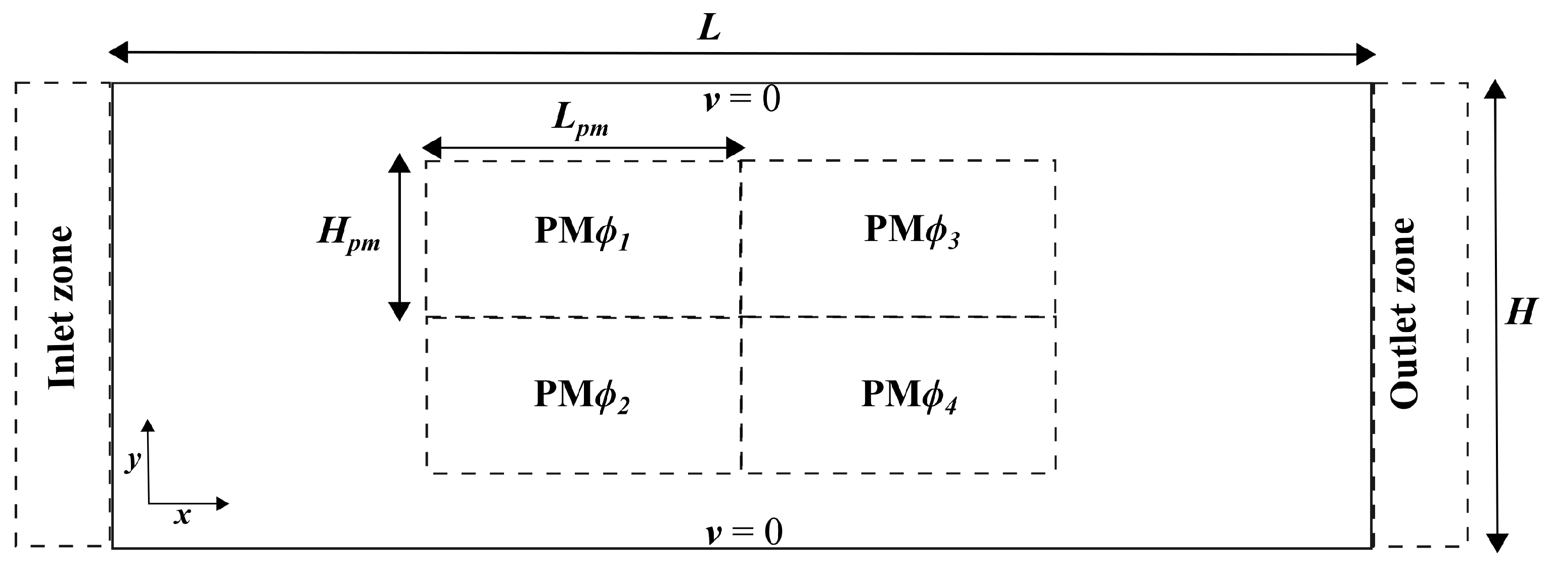
In order to maintain numerical stability, the timestep must be limited by the following partial timesteps:

$$\begin{array}{ccc}\hfill \Delta t_f& =& \underset{a}{min}\left(\sqrt{h\Vert d{\mathbf{v}}_a{/dt\Vert }^{-1}}\right),\hfill \end{array}$$

(20)

$$\begin{array}{ccc}\hfill \Delta t_{cv}& =& \underset{a}{min}{\displaystyle \frac{h}{c_{max}+{max}_b\frac{h\Vert {\mathbf{v}}_a·{\mathbf{x}}_a\Vert }{\Vert {\mathbf{x}}_a-{\mathbf{x}}_b{\Vert }^2+{ϵ}^2}}},\hfill \end{array}$$

(21)

$$\begin{array}{ccc}\hfill \Delta t_{visc}& =& 0.125{\displaystyle \frac{{\rho }_a{h}^2}{{\eta }_a}},\hfill \end{array}$$

(22)

where $\Vert d{\mathbf{v}}_a/dt\Vert$ is the magnitude of the fluid acceleration, $\eta =\rho \nu$ is the dynamic viscosity coefficient, and $c_{max}=c_0$ is the maximum artificial sound speed which enters in Equation (5). The final CFL timestep is calculated as the minimum of the above partial timesteps, i.e.,

$$\Delta t_{\mathrm{CFL}}=C_{q}min\left({\Delta }_f,\Delta t_{cv},\Delta t_{visc}\right),$$

(23)

where $C_q=0.1$.

3. Test Model

The test model consists of a truncated channel of length $L=0.2$ m and width $H=0.075$ m through which water is made to flow. As displayed in Figure 1, a heterogeneous porous layer of length $2L_{\mathrm{pm}}=0.1$ m and width $2H_{\mathrm{pm}}=0.05$ m is placed in the central core of the channel so that two clear zones are left on both sides of the substrate. At the inlet of the channel, the flow of water is assumed to be fully developed with a prescribed parabolic velocity profile. This applies to laminar flow converging to the porous layer and coming from a sufficiently long channel. In all simulations, the flowing water is assumed to be at room temperature with a density, $\rho$, and maximum inlet velocity, $v_0$, as shown in

Table 1. Physical properties of test model.

Density of Water	Inlet Velocity	Reynolds Number	Porosities
$\mathit{\rho }$	${\mathit{v}}_{\mathbf{0}}$	Re	${\mathit{\varphi }}_{\mathbf{1}}$	${\mathit{\varphi }}_{\mathbf{2}}$	${\mathit{\varphi }}_{\mathbf{3}}$	${\mathit{\varphi }}_{\mathbf{4}}$
(kg m−3)	(m s−1)
1000	$6.25\times {10}^{-3}$	46.875	0.77	0.55	0.44	0.30

. This corresponds to Reynolds number $\mathrm{Re}=46.875$. This model is an extension of previous numerical simulations for the case of a homogeneous porous substrate [11]. The heterogeneous porous layer is modeled by dividing it into four zones of different porosity (see Table 1). The same model and parameters are used for both the REV- and pore-scale calculations. For the pore-scale calculations, three different types of porous geometries are considered, consisting of regular non-staggered square (ReNoSt), regular staggered square (ReSt), and random (Ran) arrays of circular grains.

No-slip boundary conditions ($\mathbf{v}=\mathbf{0}$) are applied to the walls of the channel using the method of dynamic boundary particles, implemented in DualSPHysics [34]. This is accomplished by covering the walls of the channel with a layer of regularly spaced particles, which are used to solve for the deficiency of fluid particles near the walls. On each side of the channel, the first layer of particles is used to represent the solid wall. The boundary particles are not allowed to move, and their properties are updated by solving Equations (15) and (16) in the same way as for the fluid particles. In this way, the walls are modeled by means of a repulsive force, which is calculated by evaluating the source of Equation (16). This force is applied to the fluid particles only when they get closer than a distance of $2h$ from the walls. Across the walls, an external particle is assigned a mass, a density, and a pressure equal to the corresponding values of the wall particles, say, $m_w$, ${\rho }_w$, and $p_w$, respectively. An inlet zone is defined in front of the inlet plane by six columns of uniformly distributed particles at rest. The inlet particles carry the density of water at room temperature and velocities corresponding to a prescribed Poiseuille flow. The boundary conditions at the exit of the channel are non-reflective so that anisotropic flow can be conveyed across the outlet plane [39]. To do so, an outlet zone of particles is defined just behind the outlet plane, where the velocity vector of particles entering the outlet zone is calculated by solving the outgoing wave equation

$${\displaystyle \frac{\partial \mathbf{v}}{\partial t}}+v_x{\displaystyle \frac{\partial \mathbf{v}}{\partial x}}-\nu {\displaystyle \frac{{\partial }^2\mathbf{v}}{\partial y^2}}=\mathbf{0},$$

(24)

where $\mathbf{v}=(v_x,v_y)$ and $v_x$ is the mainstream velocity component along the channel. For particles in the outflow zone, denoted by subscript o, Equation (24) can be written in SPH form as

$${\displaystyle \frac{d{\mathbf{v}}_o}{dt}}=-v_{x,o}\sum _{b=1}^n{\displaystyle \frac{m_b}{{\overline{\rho }}_{ob}}}({\mathbf{v}}_b-{\mathbf{v}}_o){\displaystyle \frac{\partial W_{ob}}{\partial x_o}}+2\nu \sum _{b=1}^n{\displaystyle \frac{m_b}{{\rho }_b}}{\displaystyle \frac{y_{ob}({\mathbf{v}}_b-{\mathbf{v}}_o)}{\Vert {\mathbf{x}}_{ob}{\Vert }^2+{ϵ}^2}}{\displaystyle \frac{\partial W_{ob}}{\partial y_o}},$$

(25)

where ${\mathbf{x}}_{ob}={\mathbf{x}}_o-{\mathbf{x}}_b$, $y_{ob}=y_o-y_b$, and ${\overline{\rho }}_{ob}=({\rho }_o+{\rho }_b)/2$. Since outflow particles that are initially close to the outlet plane can have neighbors belonging to the fluid domain, the fluid information is advected into the outflow zone with no noise reflection back into the fluid domain. Particles within the outflow zone are moved according to the equation

$${\displaystyle \frac{d{\mathbf{x}}_o}{dt}}={\mathbf{v}}_o,$$

(26)

which must be integrated simultaneously with Equations (15)–(17) and (25).

4. Validation and Convergence Study

The SPH solver was previously tested for unsteady plane Poiseuille flow in a truncated channel (see Figure 2 of Ref. [11]). For this test, cyclic boundary conditions were employed at the entrance and exit of the channel, which favors the temporal growth of errors in the course of the calculation. In spite of this, the numerical solution was found to reproduce the exact one, with a root-mean-square error (RMSE) of less than about $5.0\times {10}^{-6}$%.

The flow of water across the channel, with a homogeneous porous layer consisting of a non-staggered array of grains with $\varphi =0.3$, is used as a convergence test. Convergence is measured by observing at which spatial resolution the REV-scale mainstream velocity profile at the exit of the channel matches the pore-scale result. In order to choose the appropriate resolution for the pore-scale simulations, the minimum spacing between grains must be known in advance in order to fill the voids with fluid particles and allow for an adequate description of the fluid flow (see Figure 2). The particles are uniformly spaced with the same inter-particle separation in the x- and y-directions (i.e., $\Delta =\Delta x=\Delta y$), and the value of h is set equal to $2\Delta$ for all runs. The channel has a width equal to $0.653H$ and a total length of $0.75L$. A homogeneous porous layer with a ReNoSt array of grains, a size of $H_{\mathrm{pm}}\times L_{\mathrm{pm}}$, and porosity of $\varphi =0.3$ is placed in the center of the channel (see Figure 3a). A value of $\varphi =0.3$ is below the range of values ($0.4\le \varphi \le 0.6$) for which the Ergun equation is applied in REV-scale simulations of fluid flow through packed beds and spherical granular materials [40].

A convergence test was performed at the pore scale by increasing the number of SPH particles from $N=\mathrm{335,532}$ to $N=\mathrm{2,998,387}$.

Table 2. The SPH parameters used for the convergence test.

Number of Particles	Inter-Particle Distance	Smoothing Length
$\mathit{N}$	$\Delta =\Delta \mathit{x}=\Delta \mathit{y}$	$\mathit{h}$
	(m)	(m)
335,532	0.00015	0.00030
751,894	0.00010	0.00020
1,530,090	0.00007	0.00014
2,998,387	0.00005	0.00010

lists the corresponding values of $\Delta$ and h. Values of h larger than $2\Delta$ resulted in more numerical diffusion and increased computational cost. The results of the runs are displayed in Figure 3b, where the velocity profiles for all three resolutions are shown at the exit of the channel. Only half of the channel width is depicted. Figure 3c is an amplification of the same profiles around the region where the velocities are higher. It is clear from this figure that asymptotic convergence is achieved when the number of SPH particles is increased from N = 751,894 to N = 1,530,090. In terms of the RMSE, the actual deviation between both curves is about $5.7\times {10}^{-6}$ m s⁻¹. The RMSE decreases further to about $3.8\times {10}^{-6}$ when the curves for N = 1,530,090 and N = 2,998,387 are compared. Based on these results, the REV- and pore-scale simulations for a heterogeneous porous medium are performed using N = 751,894 fluid particles.

5. Results

The accuracy of the REV-scale simulations to reproduce the pore-scale results for water flow through a heterogeneous porous substrate is analyzed by comparing the cross-sectional velocity profiles near the exit plane of the channel and the pressure difference across the permeable substrate.

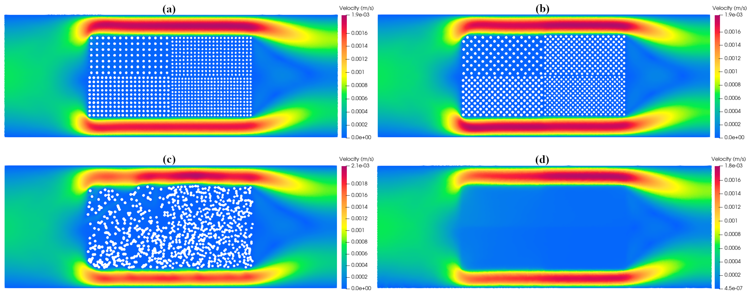
5.1. Flow Structure and Outlet Velocity Profiles

The velocity field through the channel at the pore scale for three different heterogeneous porous substrates as compared with a similar simulation at the REV scale is displayed in Figure 4. The heterogeneity of the porous substrate is constructed by joining four matrix blocks with different grain geometry and porosity. The flow structure appears to be qualitatively similar in all cases and essentially independent of the details of the porous layer (see Figure 4a–c), while the same is true when comparing the REV-scale flow field with any of the pore-scale simulations. However, there are some quantitative differences. For example, the maximum velocity along the clear zones on both sides of the porous substrate is larger in Figure 4c for random arrays of grains ($v_{max}=2.1\times {10}^{-3}$ m s⁻¹) compared to Figure 4a,b for uniformly arranged grains, where $v_{max}=1.9\times {10}^{-3}$ m s⁻¹. In contrast, at the REV scale, the maximum velocity along the clear zones is somewhat smaller (see Figure 4d), where $v_{max}=1.8\times {10}^{-3}$ m s⁻¹.

The cross-sectional velocity profiles at different stations close to the exit of the channel are displayed in Figure 5 for the same pore- and REV-scale simulation results shown in Figure 4. In particular, Figure 5a–c show the profiles at $x=0.155$ m, $x=0.18$ m, and $x=0.19$ m from the inlet plane, respectively. The heterogeneity of the porous layer affects the wave-like form of the velocity profile, which looks quite asymmetric compared to the almost symmetric form obtained for flow across a homogeneous substrate [11]. This difference in the peak velocities along the dim yellow and green streams between the right border of the substrate and the exit plane of the channel is a signature of the dependence of the flow on the non-uniform porosity and geometry of the substrate. However, in spite of differences in porosity when the grains are distributed in regular staggered arrays, the velocity profiles look much more symmetric compared to the other two geometries. Evidently, the geometric arrangement of grains in the heterogeneous porous medium influences the flow behavior through the channel. Moreover, Figure 5d displays the RMSEs between the pore- and REV-scale velocity profiles. In general, the errors are smaller than $1.0\times {10}^{-4}$ m s⁻¹, with a tendency to be even smaller when compared with the velocity profile resulting from the fluid passage through a heterogeneous porous substrate with a random distribution of grains. Lai et al. [12] performed Lattice Boltzmann calculations for the flow of water across a channel with a homogeneous porous layer in its central core, finding that for relative heights of the porous medium $2H_{pm}/H\le 0.4$, the difference in the mean mainstream velocity between the REV and pore scales is actually insignificant because most of the water flows through the clean zones adjacent to the porous layer and, therefore, the resistance of the porous substrate on the flow is negligible. However, when $2H_{pm}/H>0.4$, the difference between both scales becomes larger as $2H_{pm}/H$ increases. In particular, they found that the maximum deviations can be as large as ∼27% when $2H_{pm}/H=0.8$. In the present model, $2H_{pm}/H\approx 0.67$, and the differences in mean velocity along the channel between the REV and the pore scale are always less than about 0.01% for the three cases reported. This error is, however, similar to the one encountered when comparing the velocity profiles close to the channel exit (see Figure 5).

5.2. Pressure Losses

The pressure drop along the full channel length in the center and clear zones is displayed in Figure 6 for all three grain arrangements of the heterogeneous porous medium. A direct comparison with the pressure drop as obtained at the REV scale is provided.

Table 3. The RMSEs between the pressure drop predicted by the REV- and the pore-scale simulations. Bottom and Top refer to lines along the clear zones, while Center refers to the channel centerline.

Geometry of Grains	Position along Channel	RMSE
ReNoSt	Bottom	$1.79\times {10}^{-3}$
ReNoSt	Center	$2.87\times {10}^{-3}$
ReNoSt	Top	$1.05\times {10}^{-3}$
ReSt	Bottom	$1.45\times {10}^{-3}$
ReSt	Center	$2.29\times {10}^{-3}$
ReSt	Top	$2.72\times {10}^{-4}$
Ran	Bottom	$1.15\times {10}^{-3}$
Ran	Center	$1.64\times {10}^{-3}$
Ran	Top	$6.04\times {10}^{-4}$

lists the RMSEs between the REV- and pore-scale simulations in the center and clear zones of the channel. The deviations are always less than $2.8\times {10}^{-3}$ Pa, implying that the REV-scale simulation reproduces the pore-scale results with fairly good accuracy. In general, the pressure drop follows a qualitatively similar trend in all four cases.

An inspection of Figure 6a shows that the pressure drop predicted by the REV-scale simulation exhibits maximum deviations from any of the three pore-scale predictions in the region within the porous substrate. This is due to the very nature of the REV method, which does not aim to detail the internal phenomenology of the porous medium, but rather, models the effect of a porous medium as a homogeneous medium. In contrast, the pressure losses along the clear zones (Figure 6b,c) show little differences between the REV- and pore-scales results. Also, from Figure 6a, it follows that the pressure decay within the porous medium is not smooth due to its heterogeneity. This is a big difference with the REV-scale, where the porous matrix is assumed to be homogeneous. In spite of these small quantitative differences, these results show that the REV scale captures, with a fairly good accuracy, the trends of the pressure losses within a heterogeneous porous medium, with RMSEs that are less than about 0.3% in Pa.

6. Conclusions

The flow of water through a channel with a heterogeneous porous layer in its central core is simulated numerically using the method of Smoothed-Particle Hydrodynamics (SPH) to assess how well the flow field modeled at the Representative Elementary Volume (REV) scale with the aid of the Ergun resistance force can effectively reproduce the results at the pore scale. Since the pore-scale approach involves a much higher computational cost, it is a worthwhile task to investigate the ability of the REV scale to reproduce the flow structure and the pressure losses predicted at the pore scale. The heterogeneity of the porous medium was modeled by dividing the porous matrix into four regions that differed in the value of the porosity and distribution of their solid grains. The simulations were all performed with the aid of the latest version of the DualSPHysics hydrodynamic code [34].

The accuracy of the REV-scale simulation in reproducing the pore-scale results was measured by comparing the flow structure along the channel, the cross-sectional mainstream velocity profiles close to the exit plane of the channel, and the pressure drop through the porous substrate. It was found that the shape of the cross-sectional velocity profile after passage across the porous substrate is sensitive to both the geometric arrangement of the solid grains and the heterogeneity of the porous matrix. The REV-scale simulation was able to reproduce the mainstream velocity profiles at the pore scale to better than 0.01% using the root-mean-square error (RMSE) as a metric. Moreover, in the present simulations, the height of the porous medium relative to that of the channel was $2H_{pm}/H\approx 0.67$. For this relative height, the simulations predicted mean velocities along the channel at the REV scale that deviated from the pore-scale calculations by RMSEs of less than about 0,01%. These errors are similar to those encountered when comparing the velocity profiles close to the channel exit. In general, the pressure losses at the REV scale were also found to follow the trends predicted by the pore-scale simulations, with RMSEs of less than 0.3% in units of Pa. Since the methods and model setup employed for the REV- and pore-scale simulations are identical, they share the same level of truncation error. Therefore, by comparing the distance between the results of both models in terms of velocity and pressure losses using the RMSE as a metric, we provide a measure of the ability of the REV-scale model to reproduce the pore-scale results, implying that the SPH method can describe the flow dynamics through heterogeneous porous media at the REV scale with fairly good accuracy. This is particularly important in larger media, where high computational loads may impose serious obstacles to pore-scale simulations. Although Ergun’s model describes how the pressure losses depend upon the size of the packing, the length of bed, and the properties of the fluid, its major drawback lies in the fact that it has been formulated to particularly effectively predict head losses over packed beds of spherical grains.

References

1. Warren, J.E.; Price, H.S. Flow in heterogeneous porous media. Soc. Pet. Eng. J. 1961, 1, 153–169. [Google Scholar] [CrossRef]
2. Li, T.; Li, M.; Jing, X.; Xiao, W.; Cui, Q. Influence mechanism of pore-scale anisotropy and pore distribution heterogeneity on permeability of porous media. Pet. Explor. Dev. 2019, 46, 594–604. [Google Scholar] [CrossRef]
3. Kueper, B.H.; Abbott, W.; Farquhar, G. Experimental observations of multiphase flow in heterogeneous porous media. J. Contam. Hydrol. 1989, 5, 83–95. [Google Scholar] [CrossRef]
4. Ko, D.D.; Ji, H.; Ju, Y.S. Prediction of pore-scale flow in heterogeneous porous media from periodic structures using deep learning. AIP Adv. 2023, 13, 045324. [Google Scholar] [CrossRef]
5. Kamrava, S.; Sahimi, M.; Tahmasebi, P. Simulating fluid flow in complex porous materials by integrating the governing equations with deep-layered machines. npj Comput. Mater. 2021, 7, 127. [Google Scholar] [CrossRef]
6. Bear, J. Dynamics of Fluids in Porous Media; American Elesevier: New York, NY, USA, 1972. [Google Scholar]
7. Koekemoer, A.; Luckos, A. Effect of material type and particle size distribution on pressure drop in packed beds of large particles: Extending the Ergun equation. Fuel 2015, 158, 232–238. [Google Scholar] [CrossRef]
8. Mathias, S.A. Hydraulics, Hydrology and Environmental Engineering; Springer: Berlin, Germany, 2023. [Google Scholar]
9. Seta, T.; Takegoshi, E.; Kitano, K.; Okui, K. Thermal lattice Boltzmann model for incompressible flows through porous media. J. Therm. Sci. Technol. 2006, 1, 90–100. [Google Scholar] [CrossRef]
10. Ergun, S. Fluid flow through packed columns. Chem. Prog. 1952, 48, 89–94. [Google Scholar]
11. Alvarado-Rodríguez, C.E.; Díaz-Damacillo, L.; Plaza, E.; Sigalotti, L.D.G. Smoothed particle hydrodynamics simulations of porous medium flow using Ergun’s fixed-bed equation. Water 2023, 15, 2358. [Google Scholar] [CrossRef]
12. Lai, T.; Liu, X.; Xue, S.; Xu, J.; He, M.; Zhang, Y. Extension of Ergun equation for the calculation of the flow resistance in porous media with higher porosity and open celled-structure. Appl. Therm. Eng. 2020, 173, 115262. [Google Scholar] [CrossRef]
13. Bazmi, M.; Hashemabadi, S.H.; Bayat, M. Modification of Ergun equation for application in trickle bed reactors randomly packed with trilobe particles using computational fluid dynamics techniques. Korean J. Chem. Eng. 2011, 28, 1340–1346. [Google Scholar] [CrossRef]
14. Li, Q.; Tang, R.; Wang, S.; Zou, Z. A coupled LES-LBM-IMB-DEM modeling for evaluating pressure drop of a heterogeneous alternating-layer packed bed. Chem. Eng. J. 2022, 433, 133529. [Google Scholar] [CrossRef]
15. Li, Q.; Guo, S.; Wang, S.; Zou, Z. CFD-DEM investigation on pressure drops of heterogeneous alternative-layer particle beds for low-carbon operating blast furnaces. Metals 2022, 12, 1507. [Google Scholar] [CrossRef]
16. Turkyilmazoglu, M.; Siddiqui, A.A. The instability onset of generalized isoflux mean flow using Brinkman-Darcy-Bénard model in a fluid saturated porous channel. Int. J. Therm. Sci. 2023, 188, 108249. [Google Scholar] [CrossRef]
17. Jiang, F.; Oliveira, M.S.A.; Sousa, A.C.M. Mesoscale SPH modeling of fluid flow in isotropic porous media. Comput. Phys. Commun. 2007, 176, 471–480. [Google Scholar] [CrossRef]
18. Tartakovsky, A.M.; Ward, A.L.; Meakin, P. Pore-scale simulations of drainage of heterogeneous and anisotropic porous media. Phys. Fluids 2007, 19, 103301. [Google Scholar] [CrossRef]
19. Kunz, P.; Zarikos, I.M.; Karadimitriou, N.K.; Huber, M.; Nieken, U.; Hassanizadeh, S.M. Study of multi-phase flow in porous media: Comparison of SPH simulations with micro-model experiments. Transp. Porous Media 2016, 114, 581–600. [Google Scholar] [CrossRef]
20. Peng, C.; Xu, G.; Wu, W.; Yu, H.; Wang, C. Multiphase SPH modeling of free surface flow in porous media with variable porosity. Comput. Geotech. 2017, 81, 239–248. [Google Scholar] [CrossRef]
21. Tartakovsky, A.M.; Trask, N.; Pan, K.; Jones, B.; Pan, W.; Williams, J.R. Smoothed particle hydrodynamics and its applications for multiphase flow and reactive transport in porous media. Comput. Geosci. 2016, 20, 807–834. [Google Scholar] [CrossRef]
22. Bui, H.H.; Nguyen, G.D. A coupled fluid-solid SPH approach to modelling flow through deformable porous media. Int. J. Solids Struct. 2017, 125, 244–264. [Google Scholar] [CrossRef]
23. Lenaerts, T.; Adams, B.; Dutré, P. Porous flow in particle-based fluid simulations. ACM Trans. Graph. 2008, 27, 1–8. [Google Scholar] [CrossRef]
24. Shigorina, E.; Rüdiger, F.; Tartakovsky, A.M.; Sauter, M.; Kordilla, J. Multiscale smoothed particle hydrodynamics model development for simulating preferential flow dynamics in fractured porous media. Water Resour. Res. 2021, 57, e2020WR027323. [Google Scholar] [CrossRef]
25. Bui, H.H.; Nguyen, G.D. Smoothed particle hydrodynamics (SPH) and its applications in geomechanics: From solid fracture to granular behaviour and multiphase flows in porous media. Comput. Geotech. 2021, 138, 104315. [Google Scholar] [CrossRef]
26. Nithiarasu, P.; Seetharamu, K.N.; Sundararajan, T. Natural convective heat transfer in a fluid saturated variable porosity medium. Int. J. Heat Mass Transf. 1997, 40, 3955–3967. [Google Scholar] [CrossRef]
27. Nithiarasu, P.; Seetharamu, K.N.; Sundararajan, T. Effect of porosity on natural convective heat transfer in a fluid saturated porous medium. Int. J. Heat Fluid Flow 1998, 19, 56–58. [Google Scholar] [CrossRef]
28. Becker, M.; Teschner, M. Weakly compressible SPH for free surfaces. In Proceedings of the 2007 ACM SIGGRAPH/Europhysics Symposium on Computer Animation, San Diego, CA, USA, 2–4 August 2007; Metaxas, D., Popoovic, J., Eds.; pp. 32–58. [Google Scholar]
29. McCabe, W.L. Unit Operations of Chemical Engineering. Chemical Engineering Series; McGraw-Hill: New York, NY, USA, 2005. [Google Scholar]
30. Dukhan, N. Forced convection of nanofluids in metal foam: An essential review. Int. J. Therm. Sci. 2023, 187, 108156. [Google Scholar] [CrossRef]
31. Rabbani, A.; Jamshidi, S.; Salehi, S. Determination of specific surface of rock grains by 2D imaging. J. Geophys. Res. 2014, 2014, 945387. [Google Scholar] [CrossRef]
32. Montillet, A. Flow through a finite packed bed of spheres: A note on the limit of applicability of the Forchheimer-type equation. J. Fluids Eng. 2004, 126, 139–143. [Google Scholar] [CrossRef]
33. Venkataraman, P.; Rao, P.R.M. Validation of Forchheimer’s law for flow through porous media with converging boundaries. J. Hydraul. Eng. 2000, 126, 63–71. [Google Scholar] [CrossRef]
34. Domínguez, J.M.; Fourtakas, G.; Altomare, C.; Canelas, R.B.; Tafuni, A.; García-Feal, O.; Martínez-Estévez, I.; Mokos, A.; Vacondio, R.; Crespo, A.J.C.; et al. DualSPHysics: From fluid dynamics to multiphysics problems. Comput. Part. Mech. 2022, 9, 867–895. [Google Scholar] [CrossRef]
35. Colagrossi, A.; Landrini, M. Numerical simulation of interfacial flows by smoothed particle hydrodynamics. J. Comput. 2003, 191, 448–475. [Google Scholar] [CrossRef]
36. Bonet, J.; Lok, T.S.L. Variational and momentum preservation aspects of smoothed particle hydrodynamics formulations. Comput. Appl. Mech. Eng. 1999, 180, 97–115. [Google Scholar] [CrossRef]
37. Lo, E.Y.M.; Shao, S. Simulation of near-shore solitary wave mechanics by an incompressible SPH method. Appl. Ocean Res. 2002, 24, 275–286. [Google Scholar] [CrossRef]
38. Dehnen, W.; Aly, H. Improving convergence in smoothed particle hydrodynamics simulations without pairing instability. Mon. R. Astron. Soc. 2012, 425, 1068–1082. [Google Scholar] [CrossRef]
39. Alvarado-Rodríguez, C.E.; Klapp, J.; Sigalotti, L.D.G.; Domínguez, J.M.; de la Cruz Sánchez, E. Non-reflective outlet boundary conditions for incompressible flows using SPH. Comput. Fluids 2017, 159, 177–188. [Google Scholar] [CrossRef]
40. Zhao, C.Y. Review on thermal transport in high porosity cellular metal foams with open cells. Int. J. Heat Mass Transf. 2012, 55, 3618–3632. [Google Scholar] [CrossRef]
Figure 1. A schematic diagram of the problem.
Water 16 02801 g001
Figure 2. The uniform distribution of SPH particles inside the porous medium (filled dots) for three different numerical resolutions: (a) N = 335,532, (b) N = 751,894, and (c) N = 2,998,387. The empty circular zones represent the grains of the substrate.
Water 16 02801 g002
Figure 3. (a) The geometry of the rectangular channel with a central homogeneous porous layer used for the convergence test. (b) The cross-sectional velocity profiles for all three resolutions tried at the exit plane of the channel and (c) amplification of the same profiles around the region of maximum velocity.
Water 16 02801 g003
Figure 4. The fluid velocity field though the channel at the pore scale when the heterogeneous porous substrate is made up of (a) four ReNoSt arrays, (b) four ReSt arrays, and (c) four random arrays of circular rock grains as compared to (d) the velocity field at the REV scale.
Water 16 02801 g004
Figure 5. The cross-sectional velocity profiles near the exit of the channel at the REV and pore scales for three different geometries of the heterogeneous porous layer. Details of the flow at three different stations after passage across the porous substrate are shown (a) at x = 0.155 m, (b) at x = 0.18 m, and (c) at x = 0.19 m from the channel inlet. (d) The RMSEs as functions of the x-position between the REV- and pore-scale velocity profiles.
Water 16 02801 g005
Figure 6. The pressure losses along the full length of the channel as predicted by the REV- and pore-scale simulations when in the latter case, the porous layer consist of grains distributed in the ReNoSt, ReSt, and Ran arrays. The pressure drops are shown along (a) the centerline of the channel, (b) the top, and (c) the bottom clear zones on both sides of the heterogeneous porous layer.
Water 16 02801 g006