Abstract
Predicting the key plume evolution features of groundwater contamination are crucial for assessing uncertainty in contamination control and remediation, while implementing detailed complex numerical models for a large number of scenario simulations is time-consuming and sometimes even impossible. This work develops surrogate models with an effective and practicable pathway for predicting the key plume evolution features, such as the distance of maximum plume spreading, of groundwater contamination with natural attenuation. The representative various scenarios of the input parameter combinations were effectively generated by the orthogonal experiment method and the corresponding numerical simulations were performed by the reliable Groundwater Modeling System. The PSO-SVM surrogate models were first developed, and the accuracy was gradually enhanced from 0.5 to 0.9 under a multi-objective condition by effectively increasing the sample data size from 54 sets to 78 sets and decreasing the input variables from 25 of all the considered parameters to a smaller number of the key controlling factors. The statistical surrogate models were also constructed with the fitting degree all above 0.85. The achieved findings provide effective generic surrogate models along with a scientific basis and investigation approach reference for the environmental risk management and remediation of groundwater contamination, particularly with limited data.
1. Introduction
In recent years, the intensification of national industrial evolution and urban expansion has markedly exacerbated groundwater contamination, which may include various anthropogenic sources such as mining, smelting, and industrial activities [1,2]. Organic contaminants seep through various channels [3,4,5]. Particularly, some Southeast Asian countries are affected by the deterioration of their water environment [6,7]. Risk assessment studies has been widely applied to water environments [8]. However, the assessment of groundwater contamination risk necessitates a thorough evaluation of contributing factors to control the risk within tolerable limits, thereby facilitating the achievement of site decontamination objectives [9,10]. Natural attenuation plays a vital role in environmental restoration by leveraging processes like the convective dispersion of contaminants in groundwater and the adsorptive and degradative capacities of chemical and biological agents, thus diminishing contaminant levels [11]. Distinguished by its cost-effectiveness and minimal environmental impact, monitored natural attenuation (MNA) emerges as the foremost strategy in contemporary groundwater contamination risk management [12,13]. Accordingly, the research into predicting the plume evolution features of organic contaminants in groundwater is crucial for assessing contamination levels, refining control measures, and fostering the sustainable use of groundwater resources.
Early investigations into the natural attenuation of groundwater at contaminated sites concentrated on understanding the processes and mechanisms affecting individual contaminants. Recent studies, however, have shifted towards a quantitative analysis and predictive modeling of natural attenuation processes. Groundwater Modeling System (GMS), an advanced three-dimensional numerical modeling tool for groundwater analysis, has gained widespread and long-period adoption for assessments and predictive studies in groundwater research, providing correct simulation results with reasonable parameter settings [14,15]. Valivand and Katibrh employed GMS to develop a 3D predictive model for nitrate contamination in the groundwater of the Uruguay Plain, enhancing the precision of numerical groundwater simulations and offering a reference for further research on inorganic salt solutes in aquatic environments [16]. Similarly, Tong Xiaoxia et al. utilized GMS to identify key contaminants from a landfill site to evaluate their impact on the surrounding soil and groundwater. Their findings, derived from numerical simulations, offered crucial data and a scientific framework for mitigating water and soil pollution in landfill settings [17]. Gao Qifeng et al. applied GMS to create a model for water flow and solute transport within an industrial park, assessing the potential effects of contaminants from sewage treatment facilities on the groundwater under abnormal conditions [18]. Notably, current research often focuses on simulating the transport and fate of specific contaminants without assessing the comprehensive contamination scenarios and their future tendency. This study leverages GMS 10.4 version software simulations to statistically analyze the evolution of contamination plumes under natural attenuation conditions, and three types of data can be obtained from every simulation experiment, the distance of maximum plume spreading (DMPS), time to reach the DMPS (T-DMPS), and the mean concentration within the DMPS (MC-DMPS), which are selected to be the key features to represent every simulation scenario. These critical features are pivotal for understanding the natural attenuation process, offering vital theoretical insights and scientific contributions to the decision-making process in managing groundwater contamination risks at contaminated sites.
Surrogate models summarize uncertain or complex input–output relations through reasonable and accurate simple functions, which make an effort to reduce computational load for various large-scale complicated system research studies [19,20]. In the last few years, the continuous progression in computer technology and statistical methodologies has led to the widespread application of various statistical methods and intelligent algorithms, including multiple regression, support vector machines (SVMs), and particle swarm optimization (PSO), in environmental modeling [21,22,23,24]. For instance, Aradhi et al. incorporated a range of influential factors such as industrial activities, land use, and meteorological conditions, employing a multiple linear regression model to forecast pollution levels in the groundwater of an industrial area [25]. Muhammad et al. utilized several SVM methods for the classification and recycling application in automatic systems, elucidating the types of dry waste on solid waste and showcasing the proficiency of SVMs in complex classification challenges [26], while the optimization of kernel functions and their accompanying parameters for the SVM algorithm were not given in detail. Gai Rongli, Pang Xi, and Xu Genqi et al., by analyzing the characteristics of environmental sample data and the shortcomings of existing optimization methods, proposed the PSO-SVM algorithm to conduct research on water quality assessments by calculating the weight coefficient to determine the four main parameters with 100 sets of training data and 20 sets of testing data, air quality classification with 150 sets of training data and 215 sets of testing data after normalization processes under only one dimension, and debris flow disaster prediction with six primary inputs and 1000 sets of monitoring data. The reliability and effectiveness of the PSO-SVM model in environmental research studies with a certain number of sample data with multi-dimensional features were investigated [27,28,29]. However, there is still a lack of relevant further research on PSO-SVM modelling in groundwater environments. Wang Bilian et al. applied GMS for simulating the transport and fate from a constant pollution source within an aquifer, subsequently establishing a quantitative relationship between the characteristic variables and the related controlling factors through multiple regression analysis [30]. Nevertheless, their research did not sufficiently account for the potential influence of contamination source degradability and the characteristics of the aquitard and the confined aquifers on the plume evolution of the contaminated aquifer. Consequently, this study therefore adopts the PSO-SVM approach, takes organic contaminants as its pollution sources, and selects a more comprehensive set of factors potentially influencing the natural attenuation of groundwater contamination as input variables to conduct a further investigation. The DMPS, T-DMPS, and MC-DMPS at this juncture are employed as output variables. This methodology endeavors to develop a surrogate model for predicting the key features of the organic contamination plume evolution in groundwater environments with natural attenuation, incorporating a wider array of factors to enhance the understanding of the contaminant transport and fate dynamics.
Since the surrogate models to be developed are aimed to apply to typical groundwater systems, this paper comprehensively considers a wide range of hydrogeological and geochemical parameters that may affect the natural attenuation of the contaminant plumes. In addition, the representative various scenarios of groundwater contamination plume evolution are effectively generated by the orthogonal experiment method, and the corresponding numerical simulations are performed by the reliable Groundwater Modeling System in order to achieve the reliable basic datasets for the establishment of the surrogate models. The PSO-SVM surrogate models are first developed, and the statistical surrogate models are also constructed by multiple regression based on the same dataset used for the PSO-SVM model. Furthermore, this research endeavors to investigate model precision by enlarging the sample size and changing the input factors. A comparative evaluation between PSO-SVM models and statistical regression models is performed to offer an observation on the difference between the two types of surrogate models as to prediction accuracy performance.
2. Materials and Methods
2.1. Conceptual and Baseline Models for Constructing Different Representative Simulation Scenarios
The conceptual model for constructing different simulation scenarios was established based on a typical contaminated area which is a chemical industrial cluster in the Shandong Yellow River alluvial plain. The average annual rainfall is approximately 700 mm, and the average annual evaporation is around 1650 mm. The groundwater flows from west to east, the overall topography is flat, and the annual groundwater level change does not exceed 2 m. The region has a wide distribution and diverse types of contaminants, the concentration of part of which exceeds the corresponding water quality standards, mainly dominated by organic contaminants such as benzene and toluene.
By taking the site conditions as references, the conceptual model for this investigation was established as showed in Figure 1. The groundwater system basically consisted of, from top to bottom, the phreatic aquifer, aquitard, confined aquifer, and impermeable bottom layer. The modeling area was 7000 m × 8000 m and had a thickness of 50 m, and the corresponding grading was taken with meeting sufficient numerical computation accuracy. The hydraulic property of the groundwater system was assumed to be homogeneous and isotropous for each layer, with the fixed head boundaries on east and west sides and the specific head differences between the boundaries. In addition, groundwater contamination plume developed with a degraded contamination source in the phreatic aquifer. Furthermore, the contaminant was an easily degraded and dissolved organic compound represented by the benzene series. The contaminant transport and fate processes included advection, hydrodynamic dispersion, adsorption, and degradation. The permeability coefficient and other parameters in the baseline model were set based on the actual groundwater system, parameters, and empirical values in the investigated area, as shown in Table 1.
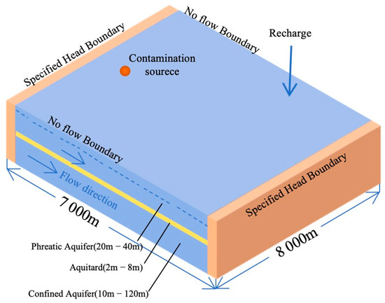
Figure 1.
Conceptual model diagram.

Table 1.
Baseline model parameters of GMS numerical simulations from the investigated site.
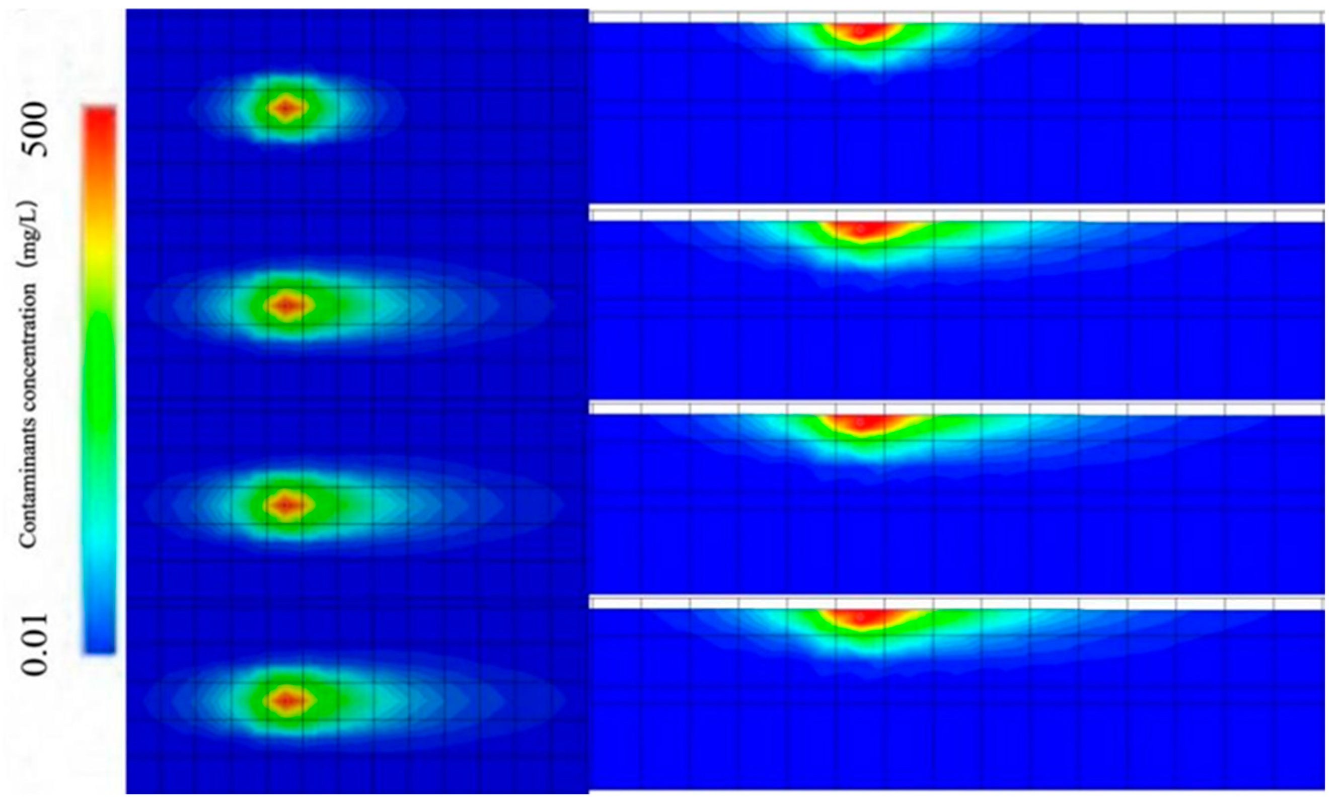
A baseline model was first established based on the investigated area for constructing the different representative simulation scenarios used for the development of the surrogate models. For the preliminary examination, typical numerical simulation results were obtained from the baseline model, shown in Figure 2. The total simulation period was set to be 40 years with a set of outputs every 180 days. In Figure 2, taking benzene as the contaminant of interest, the concentration cut-off value was set for the plume frontier as 0.01 mg/L [31].

Figure 2.
Natural attenuation of contamination plumes at 360 d, 3600 d, 7380 d, and 14,600 d of the investigated site.
2.2. Orthogonal Experiment
The orthogonal experiment, as a statistical method, is frequently used to address experimental design issues with multiple factors and levels. Its main idea is to analyze a portion of representative experimental results in order to understand the overall experimental situations [32]. By utilizing a regular orthogonal array design, representative level combinations are selected for all factors and level combinations to feature high efficiency, high speed, and economy [33].
A total of 25 parameters that impact the natural attenuation of groundwater contamination plume were selected, including the potential degradation coefficient of the contaminant source itself. Due to a multitude of parameters, an L54 (21, 324) orthogonal array was adopted to design the experimental plans according to the design rules for orthogonal experiments, with each parameter set to three levels beside the porosity of aquitard with two levels. Values for each parameter were assigned sequentially from low to high based on their possible ranges. The range of the degradation and adsorption coefficients referred to the BIOSCREEN user manual for contamination plume simulation software [34], with the maximum source concentration set above the maximum solubility of benzene contaminants (Toluene 25 °C–542 mg/L). The DMPS was calculated by counting the number of grid points with concentrations more than 0.01 mg/L in the phreatic aquifer when the contamination plume reached the farthest distance. The T-DMPS was based on the time required for the DMPS. The MC-DMPS represented the contaminant quantity per unit volume of water within the contaminated range in the phreatic aquifer. The different value levels of the 25 parameters are presented in Table 2.
Table 2.
Different value levels of each parameter set.
2.3. Support Vector Machine (SVM)
The SVM approach was established based on the VC (Vapnil Chervonenkis) dimension theory of statistical learning and the principle of minimizing structural risk. It seeks optimal results between the complexity of the model and its learning ability using limited sample information [35]. Initially introduced with the goal of finding the optimal hyperplane in the sample space, maximizing the distance between samples and the hyperplane to enhance model generalization, SVM has evolved into a prediction method employed in various classification models [36].
The SVM algorithm determines the hyperplane for classifying data points from different categories, and this hyperplane serves as a decision boundary. According to the binary classification mechanism of SVM, data points are divided into two classes defined as 0 and 1 [37]. Thus, when classifying new data points, their category can be determined based on their position relative to the hyperplane, achieving effective predictive outcomes.
For a training set, , where the sample size is l, and . Assuming , there will be errors in the prediction results inevitably represented by , and taking as the error insensitive function, then the SVM can be represented as follows:
where C and are both positive real numbers, representing the penalty factors and fitting accuracy of the control parameters respectively.
When dealing with linearly inseparable data, it is common to use kernel functions to map the features of data samples into high-dimensional space. Choosing the correct and appropriate kernel function can avoid directly computing complex calculations in high-dimensional space, thereby reflecting the results of the classification computed in low-dimensional space onto high-dimensional space. The selection of kernel functions in SVM significantly affects the predictive outcomes. Currently, commonly used kernel functions include the Sigmoid kernel function, the radial basis function (RBF), the polynomial kernel function, and the linear kernel function. Research has shown that the RBF kernel function possesses strong learning capabilities and is widely applied. Therefore, this paper selects the following RBF kernel function:
where g is the kernel parameter.
By employing the Lagrangian method, the optimization problem is transformed into its dual form:
where is the lagrange multiplier, representing the importance of each support vector.
Finally, the decision function is obtained [19].
And, the optimal solution is transformed by the following:
2.4. Optimization of SVM Parameters
SVM needs to set two parameters manually before running, penalty factor C and the kernel parameter gamma [28]. C represents the tolerance for errors, and a higher C indicates a smaller tolerance for errors, easily overfit, while a smaller C may lead to underfitting. On the other hand, the kernel parameter gamma determines the distribution of data mapped to a new feature space. The larger the gamma result, the fewer the support vectors. Therefore, the value of gamma influences the performance of training and prediction by affecting the number of support vectors.
Under the conditions of large-scale and multi-dimensional spatial data, to mitigate the impact of the penalty factor C and kernel parameter gamma on SVM, particle swarm optimization (PSO) is employed. Compared to other commonly used optimization algorithm, PSO has strong parallel processing capabilities in parameter optimization, a fast convergence speed, and global convergence advantages, and the best parameter combination of C and gamma can be searched globally [28].
The basic concept of PSO is to search for the optimal solution through cooperation and information sharing among individuals in a swarm. Each particle has only two properties, velocity and position, and each particle searches for the optimal solution in the search space individually, recording it as its personal best. By sharing individual extrema with other particles in the entire particle swarm, the optimal individual extremum is found as the current global optimal solution of the total particle swarm. All particles will change their motion speed and current position continuously based on their position relationship with the optimal particle [23]. The velocity update formula for each particle in the swarm is given by the following:
where c1 and c2 are learning factors, is the inertia factor, represents the velocity of the i-th particle, rand1 and rand2 are random numbers uniformly distributed in the interval [0,1], denotes the position of the i-th particle, and t indicates the iteration number.
The update position formula for each particle in the swarm is as follows:
The main algorithmic flow of PSO-SVM is illustrated in Figure 3.
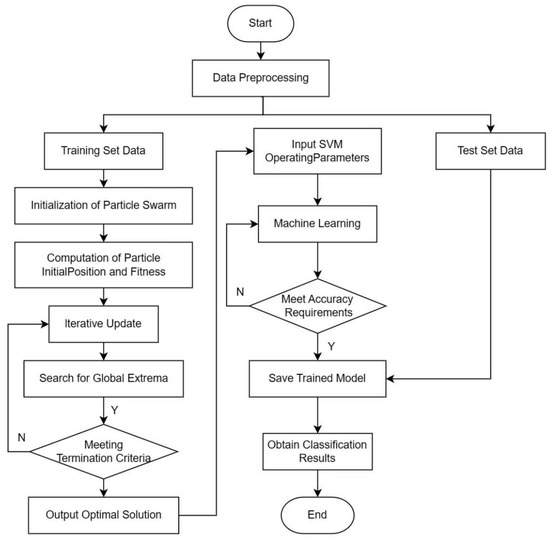
Figure 3.
PSO-SVM algorithm flowchart.
3. Results and Discussion
3.1. GMS Numerical Simulation Results of Orthogonal Experiment Scenarios
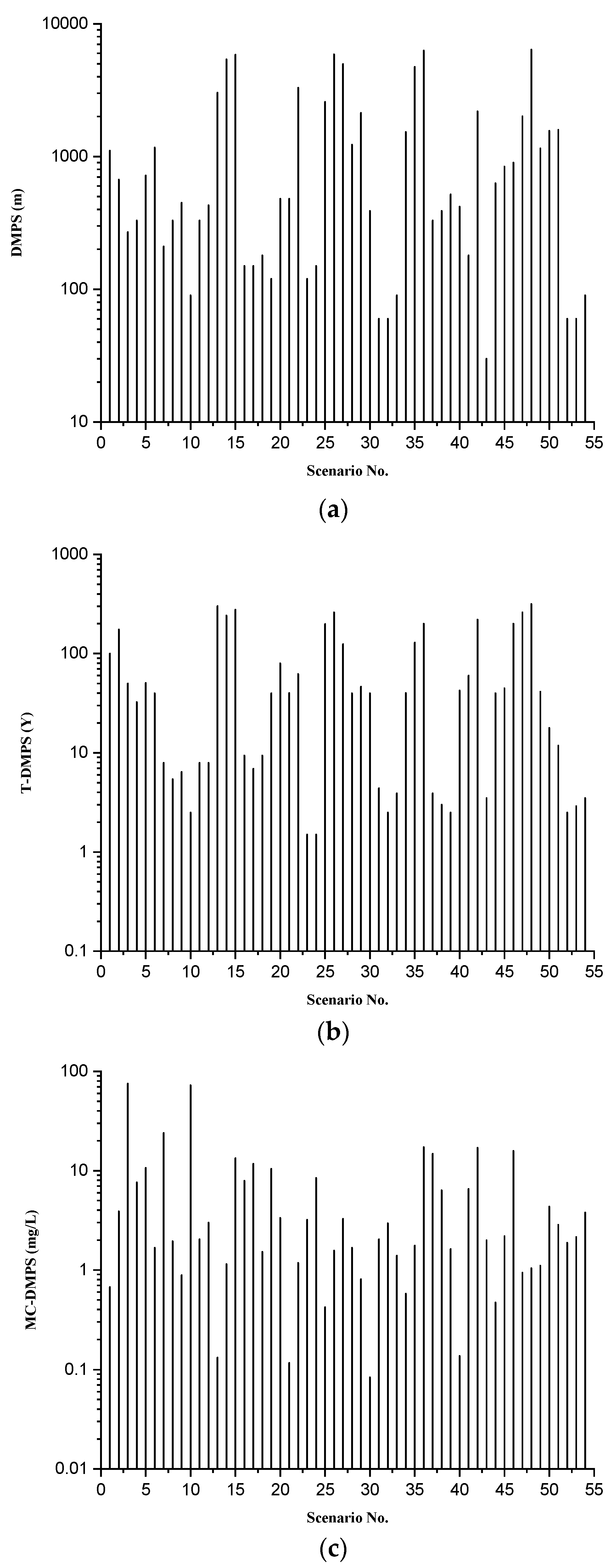
The natural attenuation process of organic contaminants in groundwater was stimulated with the investigation site, and numerous parameters were involved. Therefore, this paper employed a scenario analysis approach to explore these parameters, altering their assigned values with each set of values consistent with a specific scenario in order to generalize the prediction model of groundwater contamination plume evolution features. According to the orthogonal experiment, 54 scenarios with natural attenuation were simulated, with the simulation results represented by the key features of contaminant plume, which included the DMPS, T-DMPS, and MC-DMPS of each scenario. The experiment results of 54 sets of scenario simulation are shown in Figure 4.
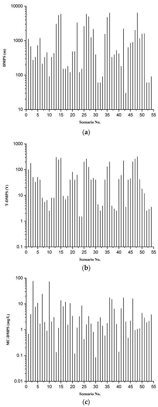
Figure 4.
The numerical simulation results from 54 representative scenarios based on the orthogonal experiment design. (a) Simulated DMPS values for 54 representative scenarios; (b) simulated T-DMPS values for 54 representative scenarios; (c) simulated MC-DMPS values for 54 representative scenarios.
3.2. Identification of Key Controlling Factors
Analysis of variance (ANOVA), a widely utilized statistical technique, is often applied to assess the differences in mean values across two or more groups, assuming the homogeneity of variance. This method divides the total variance observed within an experiment into contributions from factor effects and experimental errors, thereby offering a quantitative evaluation of the relative significance of each factor variability on the overall variation. Through F-tests conducted within the SPSS, it is possible to examine the aggregate variance attributable to the factors versus random errors, determining the factor significance on the outcomes via p-values [38]. The results show that the data meet the Bonferroni standard deviation confidence interval of 0.95 and the homogeneity of variance test, proving that all data were normally independent and with the same variance. The ANOVA findings related to the factors affecting the DMPS, T-DMPS, and MC-DMPS are presented in Table 3. Additionally, the data were performed by logarithmic transformation.
Table 3.
The total parameter analysis of variance for three different plume key features based on their individual numerical simulation results.
The ANOVA results revealed that, under the criterion of p < 0.01, there are six factors significantly associated with the T-DMPS according to the simulation outcomes: the phreatic aquifer’s effective porosity, its permeability coefficient, its adsorption coefficient, and its degradation coefficient, and the effective porosity and the adsorption coefficient of the aquitard. Regarding the DMPS, eight factors exhibit significant correlations: the head difference between the upstream and downstream boundaries, the phreatic aquifer’s permeability coefficient, its degradation coefficient, the adsorption coefficient and degradation coefficient of the aquitard, the thickness and permeability coefficient of the confined aquifer, and the concentration of the contamination source. Moreover, nine factors significantly influence the MC-DMPS: the head difference between the upstream and downstream boundaries, the phreatic aquifer’s effective porosity, its degradation coefficient, the aquitard thickness, the confined aquifer’s effective porosity, its dispersivity, the contamination source concentration, its area, and the proportion of the contamination source thickness relative to the phreatic aquifer’s thickness. With a p-value threshold set below 0.05, the count of factors significantly associated with the DMPS, T-DMPS, and MC-DMPS of the contamination plume increases to ten, nine, and fifteen, respectively.
The analysis of variance of all factors indicates that in the dynamics of groundwater contaminant natural attenuation, which encompasses the transportation, dispersion, and natural degradation of contaminants within the phreatic aquifer, there is a significant interrelation with the hydrogeological attributes of both the aquitard and the confined aquifer. This approach addresses and ameliorates the limitations observed in both domestic and international groundwater contamination studies, which often focus solely on the hydrogeological or hydrochemical parameters of phreatic aquifers.
3.3. PSO-SVM Surrogate Model
3.3.1. Model Development Based on the Dataset from Orthogonal Experiment Scenarios
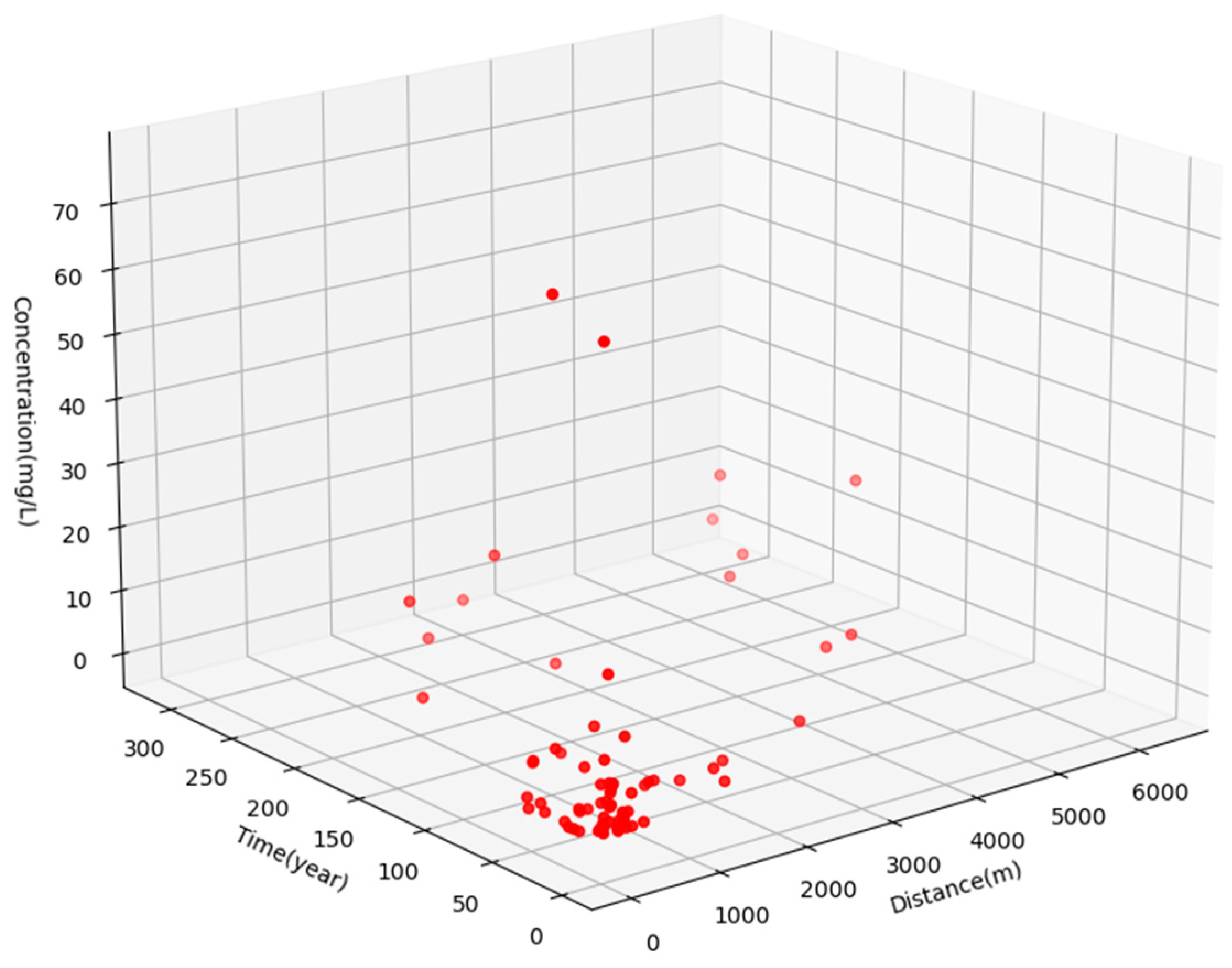
In the study on groundwater contamination plume evolution, with the natural attenuation capabilities of organic contaminants, the surrogate prediction models were developed by employing the PSO-SVM approach. Those models incorporated twenty-five variables influencing natural attenuation as input parameters, with the DMPS, T-DMPS, and MC-DMPS as their output metrics. By utilizing the classification potential of SVM, the model facilitates both single- and multi-objective predicting processes. For scenarios with a single output metric, the classification of the output data was conducted, with values above a predefined threshold marked as 0 and those below as 1, creating three distinct classification models. In addressing challenges with two output metrics, the data were paired and classified, generating three predictive models for the feature variables including the following: the DMPS, T-DMPS, and MC-DMPS. For dual-output scenarios, a two-dimensional coordinate system was employed, exemplified by the DMPS and MC-DMPS model, where the X-axis represented the MC-DMPS data and the Y-axis represented the DMPS data. This approach generated a two-dimensional dataset, marking a point as 1 when both concentration and area criteria are met and 0 otherwise, effectively converting two disparate output metrics into a binary classification challenge suitable for SVM. In cases involving three outputs for multi-objective decision making, a trio of dependent variables from simulated scenarios was plotted in a three-dimensional space, creating a dataset where the points meeting all three criteria are labeled as 1 and all others as 0. The mapping of the GMS simulation outcomes is depicted in Figure 5.

Figure 5.
The three-dimensional spatial distribution of simulation data. Each point represents a piece of data. X-axis represents T-DMPS, Y-axis represents DMPS, and Z-axis represents MS-DMPS, which means every point is a three-dimension datum under SVM calculation mechanism.
In terms of machine learning, subsequent to the data processing steps described, along with utilizing the classification mechanism inherent in support vector machines, it becomes feasible to segregate data points within two-dimensional or three-dimensional spaces by distinctly defining classification thresholds for each output parameter. For example, by establishing criteria such that the time must be less than 20 years, the distance less than 20,000 m, and the concentration less than 5 mg/L for a data point to be concurrently satisfied, such points were categorized as ‘1’, which meant class ‘1’, indicating that the plume feature performance met the specific criteria. The other plume feature performances not meeting these criteria were assigned as class ‘0’. The classification could have been changed by actual remediation targets. However, at that stage, the accuracy of the surrogate model hovered around 0.5. Consequently, efforts to improve the accuracy of the PSO-SVM model were directed towards augmenting the volume of sample data and minimizing the count of input variables.
3.3.2. Model Enhancement Based on the Additional Sample Data
The further investigation incorporated more sample data, emphasizing the scenarios primarily accounting for key controlling factors with more importance. As a result, several specific parameters associated with the source of contamination, the degradation rate Cs, initial concentration C0, and source area A were assigned two levels each. By employing a complete permutation and combination approach, eight distinct combinations were derived. These combinations, when integrated with the other parameters set at three levels within the simulation framework for the natural attenuation of groundwater contamination, culminated in a total of 24 unique scenarios. The training results are shown in Figure 6.
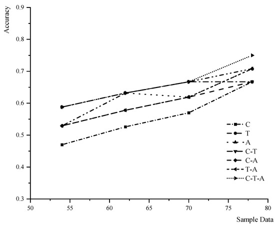
Figure 6.
The model training with sample data added.
3.3.3. Model Reliability Increasing by Dimension Deduction
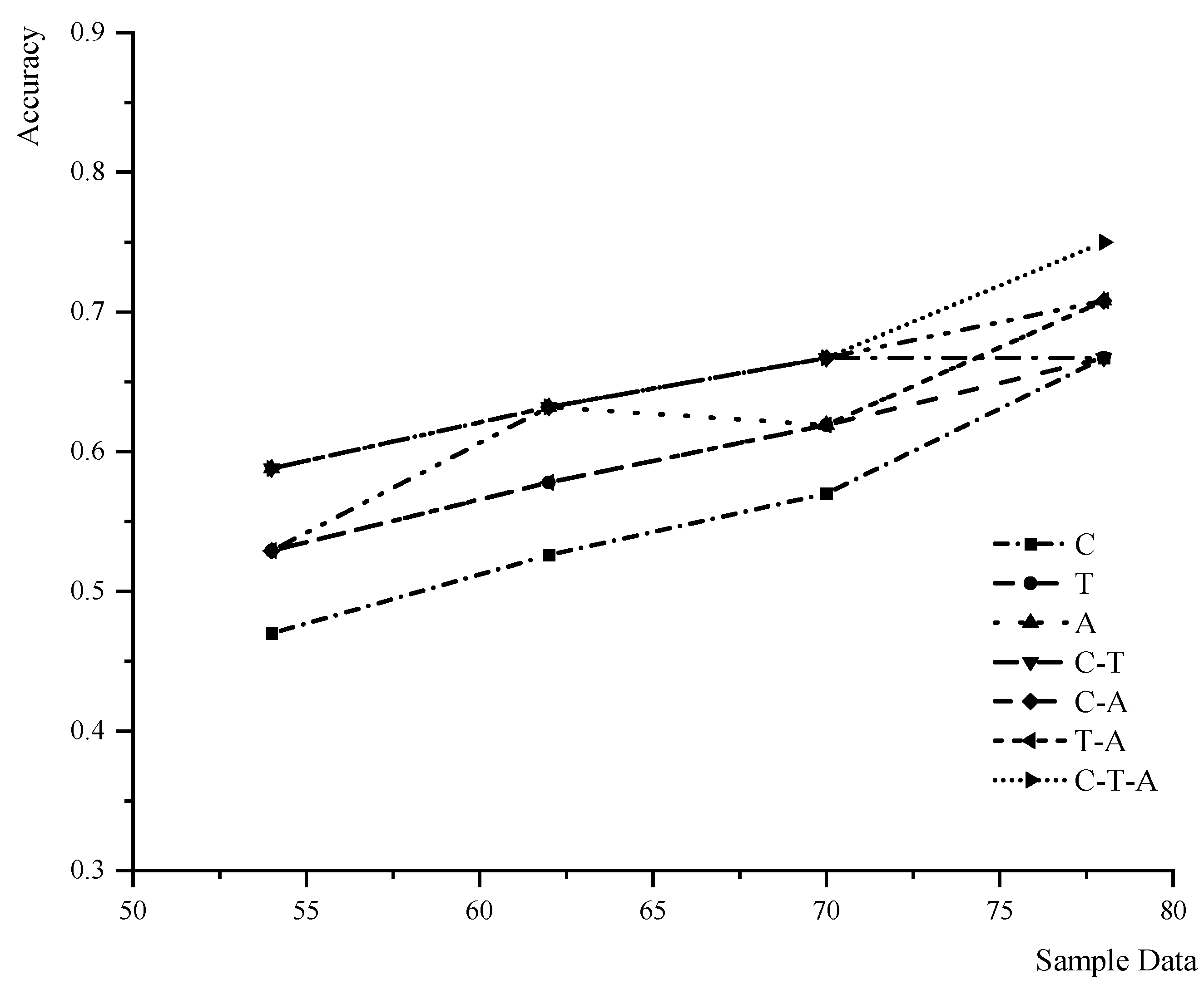
By leveraging the ANOVA results to streamline the input factors of the PSO-SVM models, the accuracy of various models was enhanced from approximately 0.5 to over 0.7. Utilizing the ANOVA results, concurrently increasing the sample size and decreasing the number of input factors, the prediction outcomes of each PSO-SVM model are detailed in the subsequent Table 4.
Table 4.
The comparison of training results from each PSO-SVM model with different outputs.
From the standpoint of model training outcomes, the implementation of critical factor selection through the application of significance values derived from the variance analysis markedly improves model accuracy. Furthermore, in the prediction model of contamination plume evolution features with multiple target outputs—namely, the DMPS, T-DMPS, and MC-DMPS—the model accuracy surpasses 0.9. Comparing with other SVM prediction or classification models, the accuracy of this surrogate model can be improved to 0.9 only with 54 sets of training data, while similar levels of accuracy were achieved by generally applying more than 100 training datasets in other reported SVM models [27,28,29].
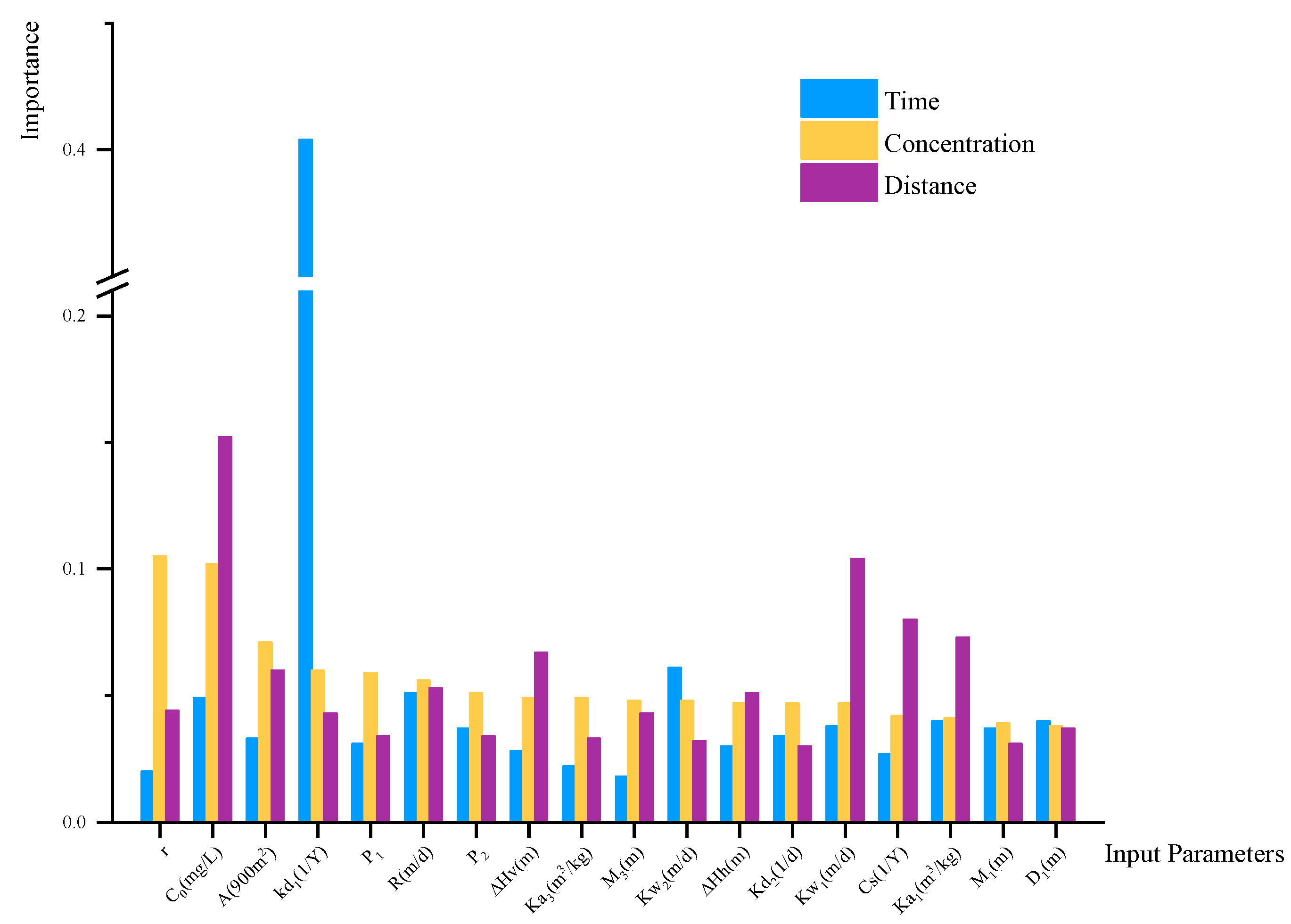
Taking the T-D-C multi-objective PSO-SVM model as an example, when analyzing the 24 test scenarios from 78 simulation scenarios, the maximum iteration step was 100. The input parameters of the three-objective model were combined with the key factors of each signal feature, so there were 20 input parameters totally. After a number of iteration steps, the particle swarm found the global optimal fitness value, indicating that the particle swarms were moving towards the optimal position after every iteration step. The importance of the input factors are presented in Figure 7. The result showed that class ‘1’ scenarios appeared 6 times, and class ‘0’ scenarios appeared 18 times. There were 22 samples of correct decisions and 2 samples of incorrect decisions, and the model accuracy was 0.917. This demonstrates the high feasibility of employing the PSO-SVM model in the research of groundwater contamination plume evolution feature prediction.
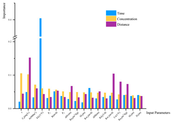
Figure 7.
The importance of input parameters.
3.4. Multiple Regression Statistical Surrogate Model
Multivariate statistical regression models are pivotal in statistical analysis, facilitating not just the exploration of the effects of several independent variables on dependent variables but also the discernment of data patterns through the examination of positive and negative correlations and the relative importance of regression coefficients among variables [39]. Additionally, these models enable the estimation and prediction of future values for dependent variables using data from existing independent variables. In this research, employing 78 simulated experimental datasets, three evolution features were considered as dependent variables (Y). A multivariate regression analysis was executed using SPSS to develop predictive statistical surrogate models for the DMPS, T-DMPS, and MC-DMPS. These models were utilized to forecast the natural attenuation of groundwater organic contamination, with the importance and significance of parameters confirmed through standard regression coefficients. The developed multivariate regression predictive model for the natural attenuation of the contaminant plume demonstrates significant predictive capability [25]. The general form of the multiple regression prediction models for the natural attenuation of contamination plumes presents as follows:
Then, the multiple regression prediction models can be transformed as follow:
where Y stands for the plume evolution features of groundwater contamination, including the DMPS, T-DMPS, and MC-DMPS.
The regression formulas for the DMPS are transformed and obtained as follows:
The regression formulas for the T-DMPS are achieved as follows:
The regression formulas for the MC-DMPS are established as follows:
Incorporating the outcomes from variance analysis, the comprehensive full-factor regression model, and the multivariate regression models with p-values above 0.05 and p-values above 0.01, the R2 values reach more than 0.85. This indicates a strong correlation between the plume evolution feature variables under natural attenuation conditions and various impact factors. The Durbin–Watson test values for the regression models are all below 2, signifying the absence of significant autocorrelation within the data and affirming the statistical significance of the models.
3.5. Discussion
3.5.1. Comparisons between the Two Types of the Developed Surrogate Models
By using an area–time–concentration multi-objective output model as an example case, selecting the same test dataset, and taking the same classification criteria as the PSO-SVM surrogate model, a comparison was performed for the model prediction accuracy between the PSO-SVM and statistical regression models. The comparison results are shown in Table 5.
Table 5.
Comparison of prediction accuracy between two types of models.
Specifically, as to the plume evolution features, the DMPS, T-DMPS, and MC-DMPS, a study case was established using the same test data and classification criteria as those applied in both PSO-SVM and statistical regression models, followed by an accuracy comparison. The comparison findings indicated that with contamination plume thresholds defined as a DMPS under 2000 m, T-DMPS below 20 years, and MC-DMPS less than 5 mg/L, the accuracy of the regression model for multiple outputs stood at 0.75. Nonetheless, the accuracy of the regression surrogate models experienced a notable decline with the identified key controlling factors, rendering the performance generally inferior to or at best comparable to that of the PSO-SVM surrogate model. This stressed the superior performance of the PSO-SVM model when operating with a limited number of key controlling factors. By taking the data volume into consideration, the PSO-SVM surrogate model also offered a good performance based on a limited dataset, which meant this surrogate mode took a wider application in situations where the data were laborious to obtain. In addition, it was indicated that the PSO-SVM model could achieve more accurate results under conditions of limited parameter availability compared to the conventional statistical approaches, while other published research studies were less focused on the comparison between different types of prediction models based on the same test data [17,18,19]. Overall, the PSO-SVM surrogate model demonstrated greater reliability of application for predicting plume evolution features concerning groundwater contamination, particularly regarding the natural attenuation of organic contaminants with a limited data size, than the traditional regression models.
3.5.2. Further Elucidation about the Validation on the Built Surrogate Models
The statistical surrogate models and PSO-SVM surrogate models were both built up based on the datasets from the numerical simulation results, obtained through the reliable Groundwater Modeling System, of many representative modeling scenarios. This means that the numerical simulation data used in this investigation can be treated as the “real accurate data” for establishing those surrogate models. As a result, we should firstly validate our surrogate models using additional numerical simulation data from the representative modeling scenarios which were not included and utilized for building the surrogate models. In fact, in this investigation, we conducted validation tests, by using an additional 24 datasets, on both the statistical surrogate models and PSO-SVM surrogate models. In this sense, we would say that our surrogate models have been tested in respect to the real prediction of experimental results. Certainly, it is reasonable and valuable to perform further examinations and confirmations on those established surrogate models using the specific site field data in future practical applications.
3.5.3. Practicability and Advantage of Prediction Uncertainty Assessment
Upon considering the uncertainty in obtaining the factor parameter values, there are different degrees of uncertainty regarding the predicted results of plume evolution feature variables. The uncertainty analyses by Monte Carlo simulations can evaluate the possible range of variation for the prediction results obtained from the established surrogate models. Therefore, giving the parameter error range of related impact factor variables and their distribution types, a large number of possible different parameter combination scenarios (such as 500 scenarios) can be generated. By using the surrogate models, the prediction results of corresponding plume feature variables for all the scenarios can be efficiently calculated, and the relative frequency distribution histogram of the predicted results can be rapidly obtained. Based on the relative frequency distribution histogram, under a given confidence probability, the possible variation range of the plume feature variables can be offered quickly, providing a quantitative basis for the upper and lower boundaries of plume feature variables in contamination control and risk management decision making. Comparably, it is time-consuming, even impossible, to implement detailed complex numerical models since a large number of simulations of scenarios are required.
4. Conclusions
This work developed surrogate models with an effective and practicable pathway for predicting the key plume features, including the DMPS, T-DMPS, and MC-DMPS, of groundwater contamination with natural attenuation. The developed models were aimed to apply to typical groundwater systems, and a wide range of the hydrogeological and geochemical parameters were comprehensively considered that may affect the natural attenuation of the contaminant plumes. The main conclusions drawn from this investigation are given as follows:
- (1)
- According to the numerical simulations and variance analysis, the key controlling factors affecting the DMPS, T-DMPS and MC-DMPS of contaminant plumes are different. It is indicated that the transport and fate of contaminants in the aquifer are significantly correlated not only with hydrological parameters but also with certain parameters of the aquitard and confined aquifer. The degradation coefficient of the phreatic aquifer is a crucial factor determining the natural attenuation of the contaminants.
- (2)
- The PSO-SVM model prediction accuracy can be gradually enhanced by implementing the measures of effectively increasing the sample data sizes and replacing all of considered input variables with the identified key controlling factors. It is interesting to note that the final developed PSO-SVM models still can present good reliability with the utilization of the limited sample data.
- (3)
- The statistical surrogate models are also constructed by multiple regression based on the same dataset used for the PSO-SVM model. The statistical regression surrogate models also exhibit pretty good fitting accuracy, while in comparison, the PSO-SVM models offer generally higher prediction accuracy than the statistical regression models, particularly by taking the key controlling factors as input variables.
- (4)
- The findings of this study offer effective generic surrogate models along with a scientific basis and investigation approach reference for environmental risk management and remediation pertaining to the commonly existing groundwater contamination.
Author Contributions
Conceptualization, Y.W. and M.W.; methodology Y.W. and M.W.; software, Y.W. and R.L.; formal analysis, Y.W. and M.W.; writing—original draft preparation, Y.W.; writing—review and editing, M.W.; supervision, M.W.; project administration, M.W.; funding acquisition, M.W. All authors have read and agreed to the published version of the manuscript.
Funding
This research was supported by the National Key Research and Development Program of China (2020YFC1807102, 2020YFC1807100).
Data Availability Statement
Data are contained within the article.
Conflicts of Interest
The authors declare no conflicts of interest.
References
- Demirak, A.; Yilmaz, F.; Tuna, A.L.; Ozdemir, N. Heavy metals in water, sediment and tissues of Leuciscus cephalus from a stream in southwestern Turkey. Chemosphere 2006, 63, 1451–1458. [Google Scholar] [CrossRef] [PubMed]
- Muhammad, S.; Shah, M.T.; Khan, S. Arsenic health risk assessment in drinking water and source apportionment using multivariate statistical techniques in Kohistan region, northern Pakistan. Food Chem. Toxicol. 2010, 48, 2855–2864. [Google Scholar] [CrossRef]
- Wang, W.; Jia, J.; Zhang, B.; Xiao, B.; Yang, H.; Zhang, S.; Gao, X.; Han, Y.; Zhang, S.; Liu, Z.; et al. A review of Sustained release materials for remediation of organically contaminated groundwater: Material preparation, applications and prospects for practical application. J. Hazard. Mater. Adv. 2024, 13, 100393. [Google Scholar] [CrossRef]
- Cundy, A.; Bardos, R.; Church, A.; Puschenreiter, M.; Friesl-Hanl, W.; Müller, I.; Neu, S.; Mench, M.; Witters, N.; Vangronsveld, J. Developing principles of sustainability and stakeholder engagement for “gentle” remediation approaches: The European context. J. Environ. Manag. 2013, 129, 283–291. [Google Scholar] [CrossRef] [PubMed]
- Ravindiran, G.; Rajamanickam, S.; Sivarethinamohan, S.; Sathaiah, B.K.; Ravindran, G.; Muniasamy, S.K.; Hayder, G. A Review of the Status, Effects, Prevention, and Remediation of Groundwater Contamination for Sustainable Environment. Water 2023, 15, 3662. [Google Scholar] [CrossRef]
- Hossain, M.; Bhattacharya, P.; Jacks, G.; von Brömssen, M.; Ahmed, K.M.; Hasan, M.A.; Frape, S.K. Sustainable Arsenic Mitigation–from Field Trials to Implementation for Control of Arsenic in Drinking Water Supplies in Bangladesh. Best Practice Guide on the Control of Arsenic in Drinking Water; Metals and Related Substances in Drinking Water Series; IWA Publishing: London, UK, 2017; pp. 99–116. [Google Scholar]
- Lone, S.A.; Jeelani, G.; Mukherjee, A.; Coomar, P. Arsenic fate in upper Indusr iver basin (UIRB) aquifers: Controls of hydrochemical processes, provenances and water-aquifer matrix interaction. Sci. Total Environ. 2021, 795, 148734. [Google Scholar] [CrossRef]
- Qaiser, F.U.; Zhang, F.; Pant, R.R.; Zeng, C.; Khan, N.G.; Wang, G. Characterization and health risk assessment of arsenic in natural waters of the Indus River Basin, Pakistan. Sci. Total Environ. 2023, 857, 159408. [Google Scholar] [CrossRef]
- Liu, G.; Niu, J.; Zhang, C.; Guo, G. Characterization and assessment of contaminated soil and groundwater at an organic chemical plant site in Chongqing, Southwest China. Environ. Geochem. Health 2016, 38, 607–618. [Google Scholar] [CrossRef]
- Bardos, R.P.; Bone, B.D.; Boyle, R.; Evans, F.; Harries, N.D.; Howard, T.; Smith, J.W. The rationale for simple approaches for sustainability assessment and management in contaminated land practice-ScienceDirect. Sci. Total Environ. 2016, 563, 755–768. [Google Scholar] [CrossRef]
- Li, Y.; Wang, S.; Zhang, M.; He, Z.; Zhang, W. Research progress of monitored natural attenuation remediation technology for soil and groundwater pollution. Zhongguo Huanjing Kexue/China Environ. Sci. 2018, 38, 1185–1193. [Google Scholar]
- U.S. Environmental Protection Agency. Use of Monitored Natural Attenuation at Superfund, RCRA, Corrective Action and UST Sites EPA’s Office of Solid Waste and Emergency Response (OSWER) Directive 9200.4-17; U.S. Environmental Protection Agency: Washington, DC, USA, 1999.
- Rügner, H.; Finkel, M.; Kaschl, A.; Bittens, M. Application of monitored natural attenuation in contaminated land management—A review and recommended approach for Europe. Environ. Sci. Policy 2006, 9, 568–576. [Google Scholar] [CrossRef]
- Amiri, S.; Rajabi, A.; Shabanlou, S.; Yosefvand, F.; Izadbakhsh, M.A. Prediction of groundwater level variations using deep learning methods and GMS numerical model. Earth Sci. Inform. 2023, 16, 3227–3241. [Google Scholar] [CrossRef]
- Valivand, F.; Katibeh, H. Simulation and Prediction of Groundwater Pollution Based on GMS: A Case Study in Beijing, China. IOP Conf. Ser. Earth Environ. Sci. 2021, 826, 012014. [Google Scholar]
- Valivand, F.; Katibeh, H. Prediction of nitrate distribution process in the groundwater via 3D modeling. Environ. Model. Assess. 2020, 25, 187–201. [Google Scholar] [CrossRef]
- Tong, X.X.; Ning, L.B.; Dong, S.G. GMS model for assessment and prediction of groundwater pollution of a garbage dumpling site in Luoyang. Miner. Explor. 2012, 35, 197–201. [Google Scholar]
- Gao, Q.F.; Jiao, J.N.; Zhang, Y.Z.; Du, J.X. Application of numerical simulation in groundwater environmental impact assessment based on GMS: A case study of an industrial park. Miner. Explor. 2023, 14, 1236–1243. [Google Scholar]
- Zou, Y.; Yousaf, M.S.; Yang, F.; Deng, H.; He, Y. Surrogate-Based Uncertainty Analysis for Groundwater Contaminant Transport in a Chromium Residue Site Located in Southern China. Water 2024, 16, 638. [Google Scholar] [CrossRef]
- Davis, S.E. Efficient Surrogate Model Development: Impact of Sample Size and Underlying Model Dimensions. Comput. Aided Chem. Eng. 2018, 44, 979–984. [Google Scholar]
- Kanu, O.P.; Ugwoha, E.; Udeh, N.U.; Amah, V. Modelling Groundwater Quality of Aba in Abia State Using Principal Component Analysis and Multiple Linear Regression. J. Eng. Res. Rep. 2023, 25, 39–54. [Google Scholar] [CrossRef]
- Alshahri, A.H.; Elbisy, M.S. Assessment of Using Artificial Neural Network and Support Vector Machine Techniques for Predicting Wave-Overtopping Discharges at Coastal Structures. J. Mar. Sci. Eng. 2023, 11, 539. [Google Scholar] [CrossRef]
- Guneshwor, L.; Eldho, T.I.; Kumar, A.V. Identification of Groundwater Contamination Sources Using Meshfree RPCM Simulation and Particle Swarm Optimization. Water Resour. Manag. 2018, 32, 1517–1538. [Google Scholar] [CrossRef]
- Gad, M.; Gaagai, A.; Eid, M.H.; Szűcs, P.; Hussein, H.; Elsherbiny, O.; Elsayed, S.; Khalifa, M.M.; Moghanm, F.S.; Moustapha, M.E.; et al. Groundwater Quality and Health Risk Assessment Using Indexing Approaches, Multivariate Statistical Analysis, Artificial Neural Networks, and GIS Techniques in El Kharga Oasis, Egypt. Water 2023, 15, 1216. [Google Scholar] [CrossRef]
- Krishna, A.K.; Satyanarayanan, M.; Govil, P.K. Assessment of heavy metal pollution in water using multivariate statistical techniques in an industrial area: A case study from Patancheru, Medak District, Andhra Pradesh, India. J. Hazard. Mater. 2009, 167, 366–373. [Google Scholar] [CrossRef] [PubMed]
- Nuzul, N.B.M.; Hassan, M.K.; Norrima, M.; Amirul, W.M.W.; Heshalini, R.; Tarmizi, A.; Jafferi, J. Automatic dry waste classification for recycling purpose. Int. Conf. Artif. Life Robot. 2022, 3, 1003–1010. [Google Scholar]
- Gai, R.; Guo, Z. A water quality assessment method based on an improved grey relational analysis and particle swarm optimization multi-classification support vector machine. Front. Plant Sci. 2023, 14, 1099668. [Google Scholar] [CrossRef]
- Pang, X.; Hu, H.R.; Zhao, C.; Bai, N.B. Research on air quality classification based on PSO-SVM algorithm. Environ. Sci. Surv. 2023, 42, 63–67. [Google Scholar]
- Xu, G.; Yan, X.-E.; Cao, N.; Ma, J.; Xie, G.; Li, L. Debris Flow Prediction Based on the Fast Multiple Principal Component Extraction and Optimized Broad Learning. Water 2022, 14, 3374. [Google Scholar] [CrossRef]
- Wang, B.L.; Wang, M.Y.; Pang, Y.T. Primary controlling Factors and statistical modeling of plum stability for BTEX in Typical phreatic aquifers. Earth Sci. 2023, 48, 3454–3465. [Google Scholar]
- GBT 14848-2017; Quality Standard for Groundwater. Standardization Administration of the People’s Republic of China: Beijing, China, 2017.
- Vapnik, V. The Natural of Statistical Learning Theory; Springer Science & Business Media: Berlin/Heidelberg, Germany, 1995. [Google Scholar]
- Samandi, V.; Mukhopadhyay, D. Workflow scheduling in cloud computing environment with classification ordinal optimisation using SVM. Int. J. Comput. Sci. Eng. 2021, 24, 563–571. [Google Scholar] [CrossRef]
- Fan, Z.; Chen, W.G.; Zou, J.X.; Yang, D.K.; Shi, H.Y. Quantitative Analysis of Furfural Dissolved in Transformer Oil Based on Raman Spectroscopy. J. Light Scatt. 2018, 30, 46–50. [Google Scholar]
- Li, M.Z.; Zhai, Y.Z.; Zuo, R. Sensitivity Analysis of Parameters in Numerical Simulation of Solute Transport in Groundwater. S.-N. Water Transf. Water Sci. Technol. 2014, 3, 133–137. [Google Scholar]
- Zhang, S.; Liu, Z.; Sun, R.; Liu, W.; Chen, Y. Orthogonal Experimental Study on Remediation of Ethylbenzene Contaminated Soil by SVE. Sustainability 2023, 15, 1168. [Google Scholar] [CrossRef]
- Newell, C.J.; Mcleod, R.K.; Gonzales, J.R. BIOSCREEN: Natural Attenuation Decision Support System. User’s Manual Version 1.3; U.S. Environmental Protectin Protection Agency, Office of Research and Development: Washington DC, USA, 1996.
- Ni, H.; Liu, Y.R.; Long, Z.G. Application of orthogonal design to sensitivity analysis of landslide. Chin. J. Rock Mech. Eng. 2002, 21, 989–992. [Google Scholar]
- Li, L. Quantifying TiO2 Abundance of Lunar Soils: Partial Least Squares and Stepwise Multiple Regression Analysis for Determining Causal Effect. J. Earth Sci. 2011, 22, 549–565. [Google Scholar] [CrossRef]


Disclaimer/Publisher’s Note: The statements, opinions and data contained in all publications are solely those of the individual author(s) and contributor(s) and not of MDPI and/or the editor(s). MDPI and/or the editor(s) disclaim responsibility for any injury to people or property resulting from any ideas, methods, instructions or products referred to in the content. |
© 2024 by the authors. Licensee MDPI, Basel, Switzerland. This article is an open access article distributed under the terms and conditions of the Creative Commons Attribution (CC BY) license (https://creativecommons.org/licenses/by/4.0/).