

Temperature and Precipitation Change Assessment in the North of Iraq Using LARS-WG and CMIP6 Models


Abstract
:1. Introduction
- To apply the LARS-WG (8) technique to project climatic factors (i.e., rainfall and temperature) over the period (2021–2040) covering fifteen meteorological locations in the north of Iraq.
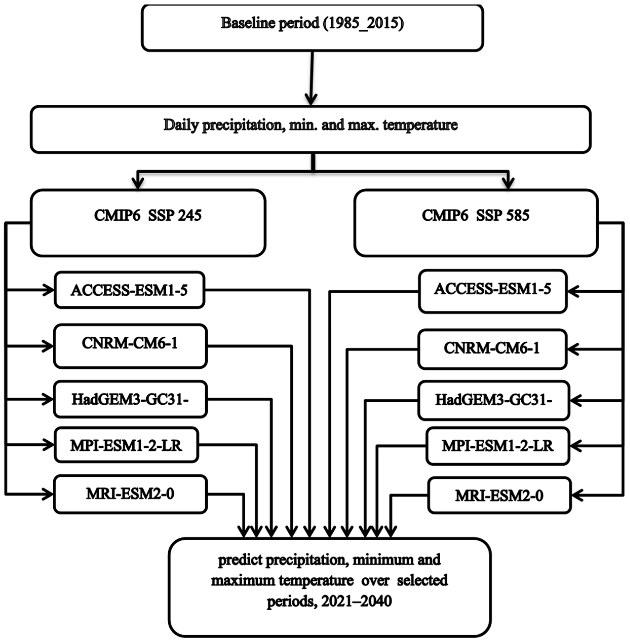
- To assess the impact of two climate scenarios (i.e., SSP245 and SSP585) by integrating CMIP6 predictions from five GCMs to capture a wide variety of possible results and to lessen the uncertainty surrounding future predictions.
- To examine the projected and historical spatial-temporal seasonal variability of rainfall and mean temperature to discover the potential effects of future SSP245 and SSP585 scenarios.
- To contribute essential information for environmental planning at the local level, focusing on the management of water resources and the reduction of hazards associated with extreme hydrological occurrences in the near to medium term (2021–2040).
2. Materials and Methods
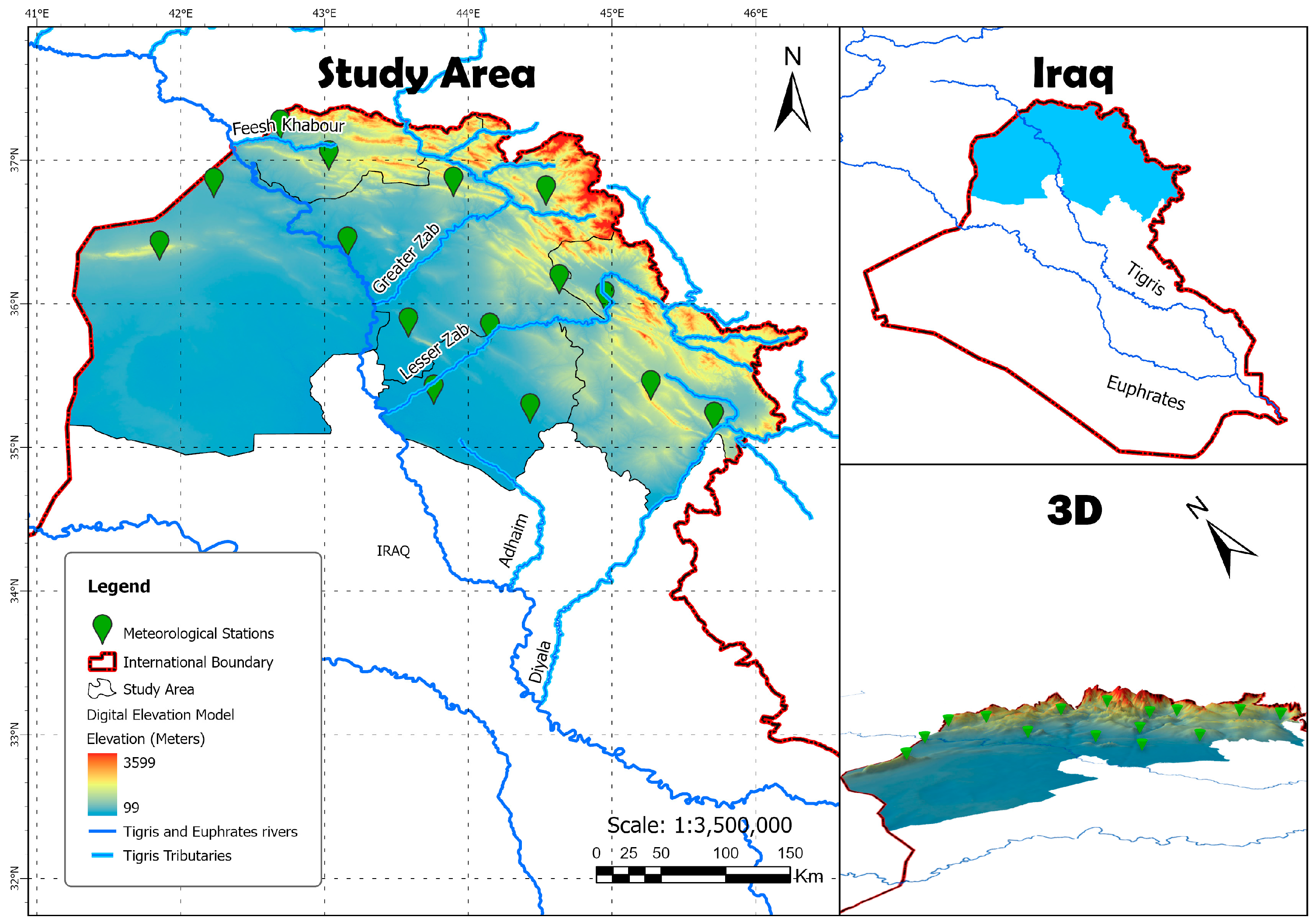
2.1. Area of the Study and the Data Set
2.2. Downscaling Using LARS-WG
3. Results
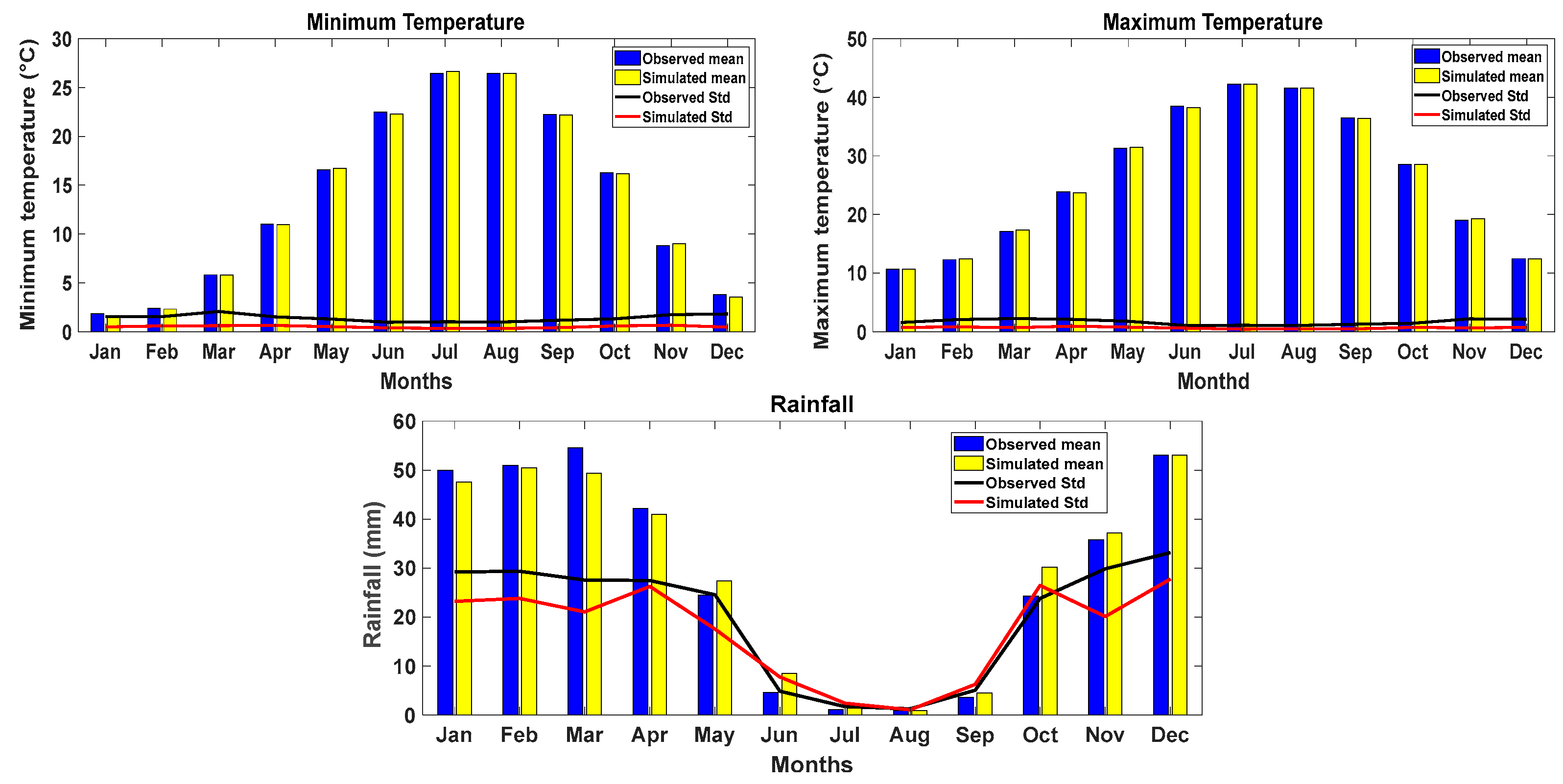
3.1. Calibration and Validation of the Model
3.2. Projection Results
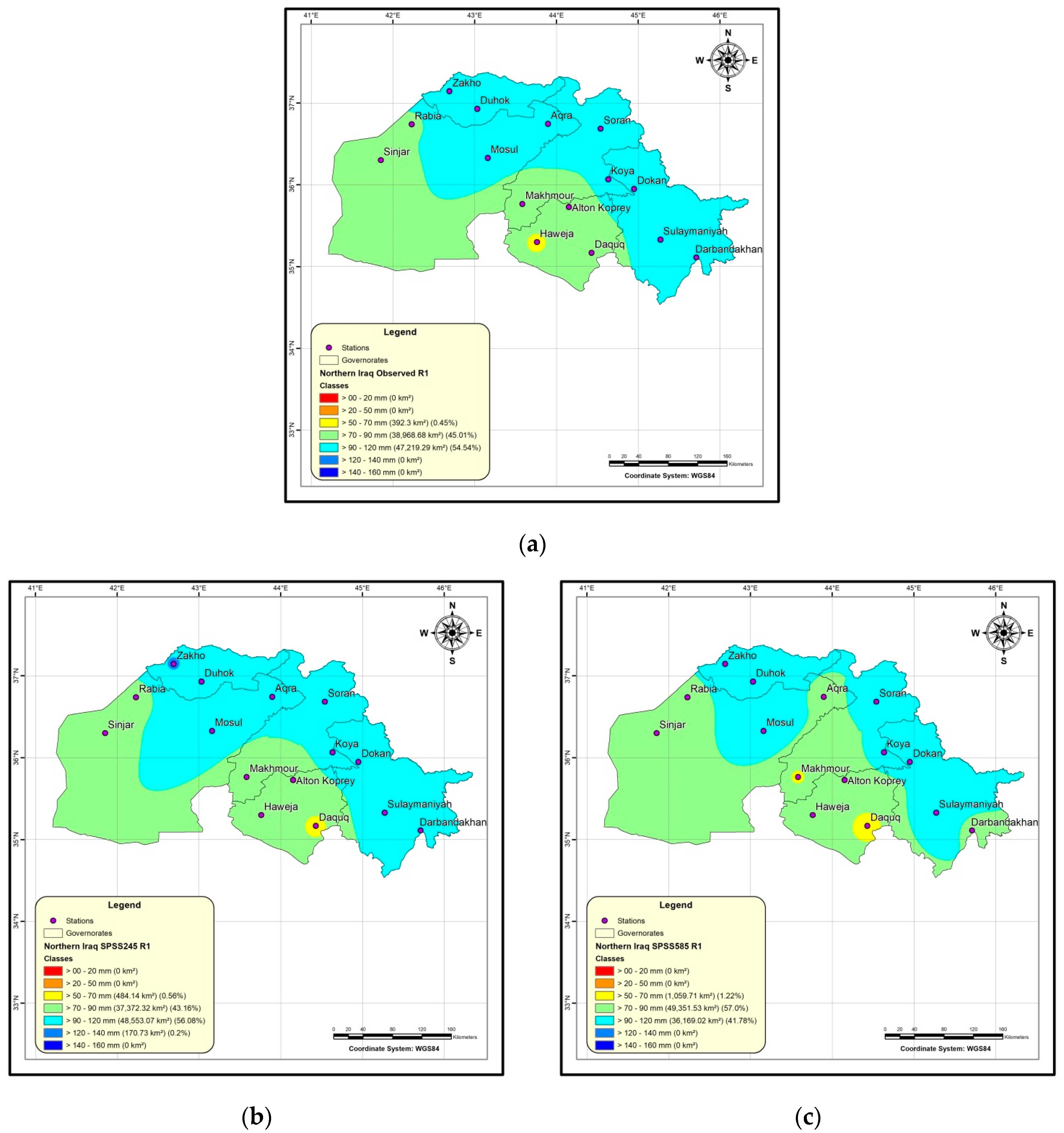
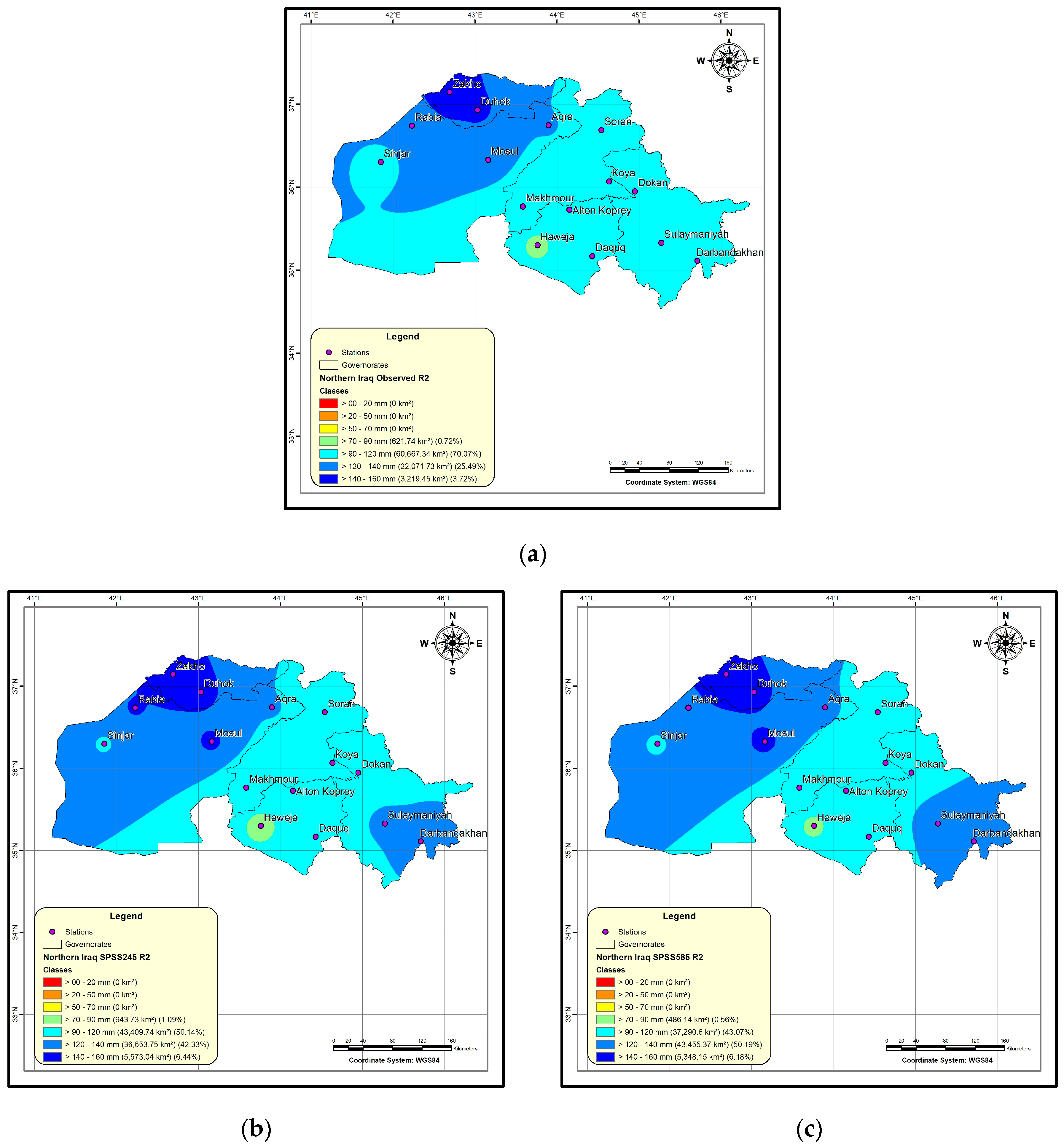
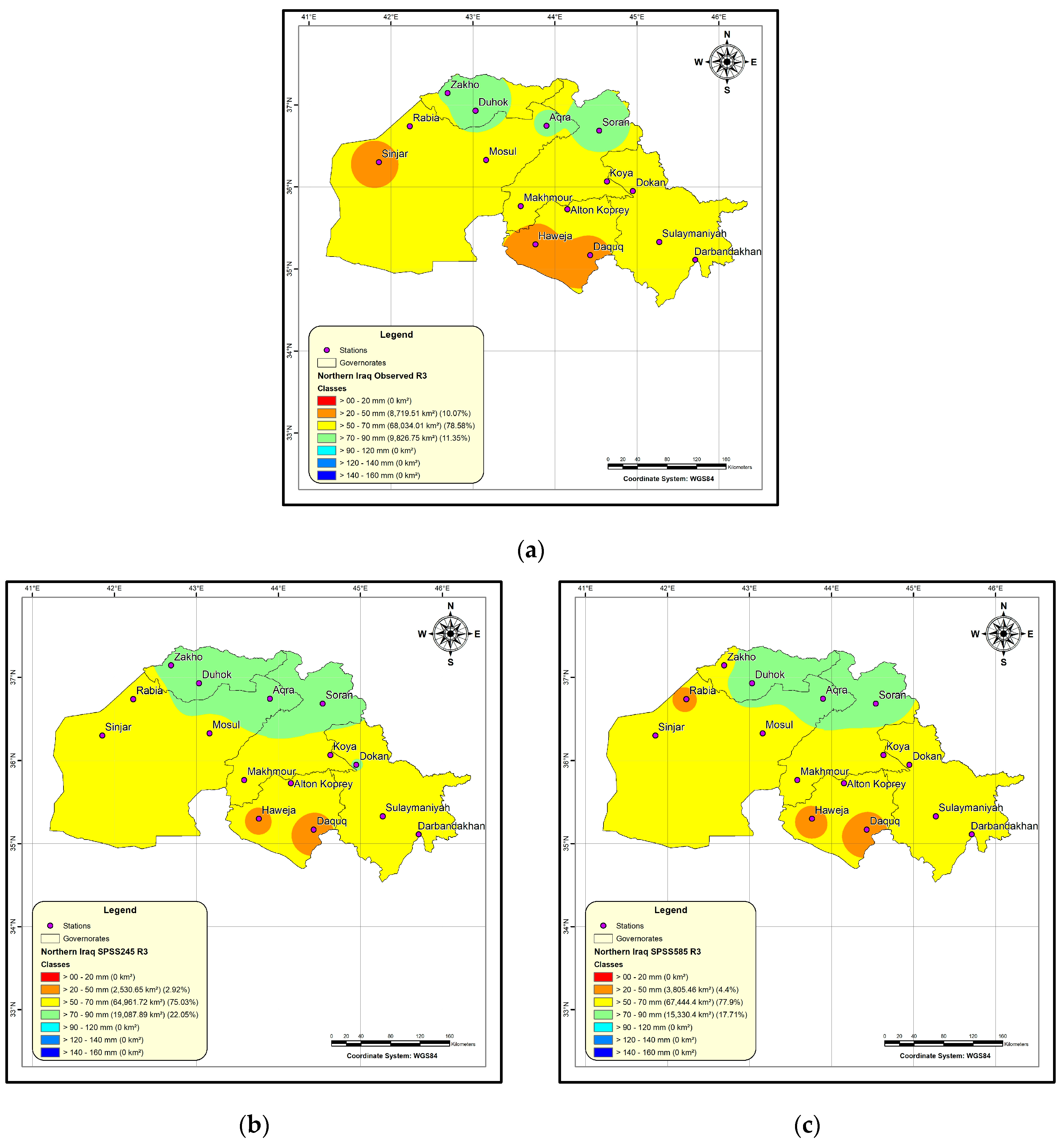
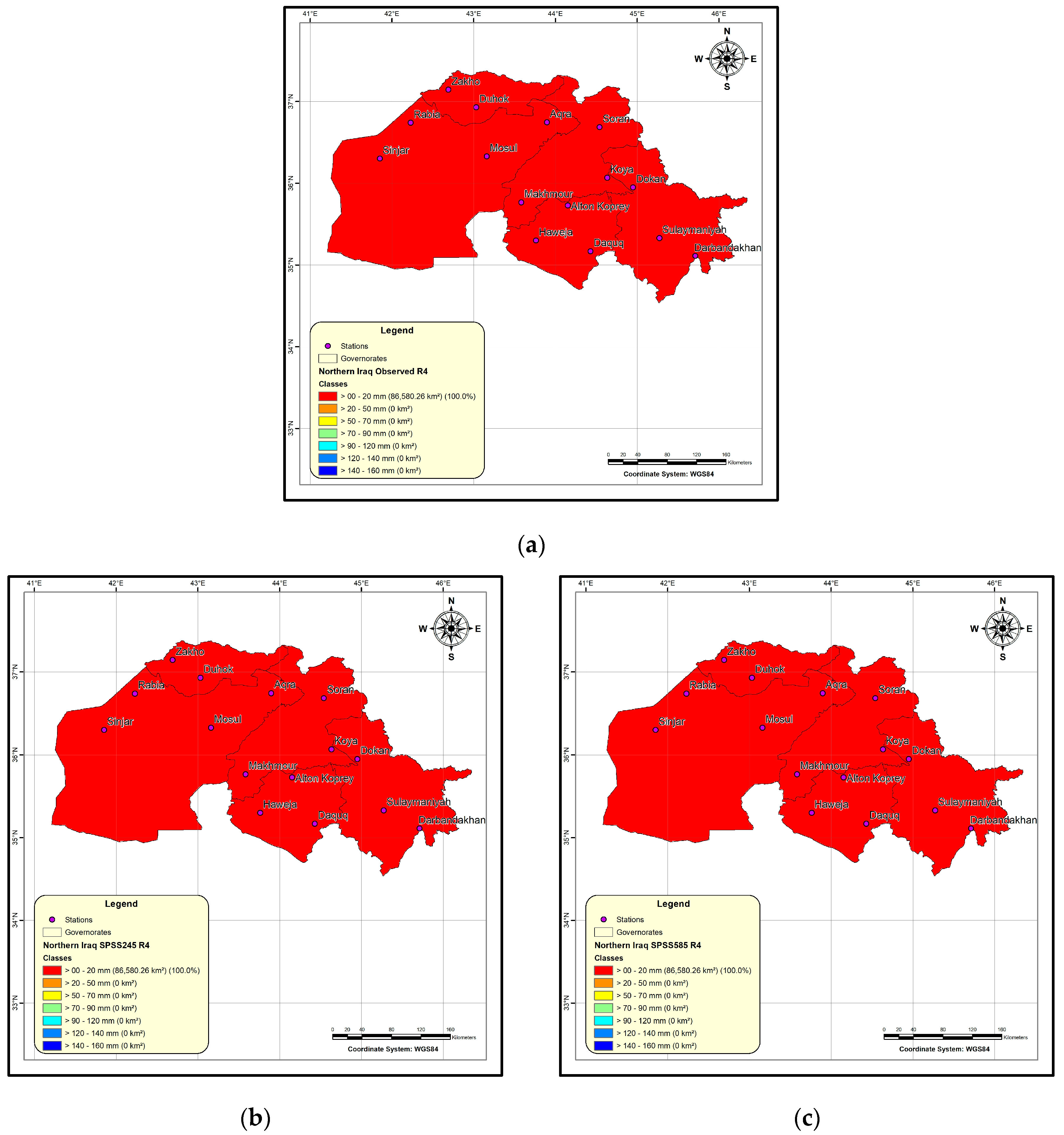
3.2.1. Projection of Precipitation
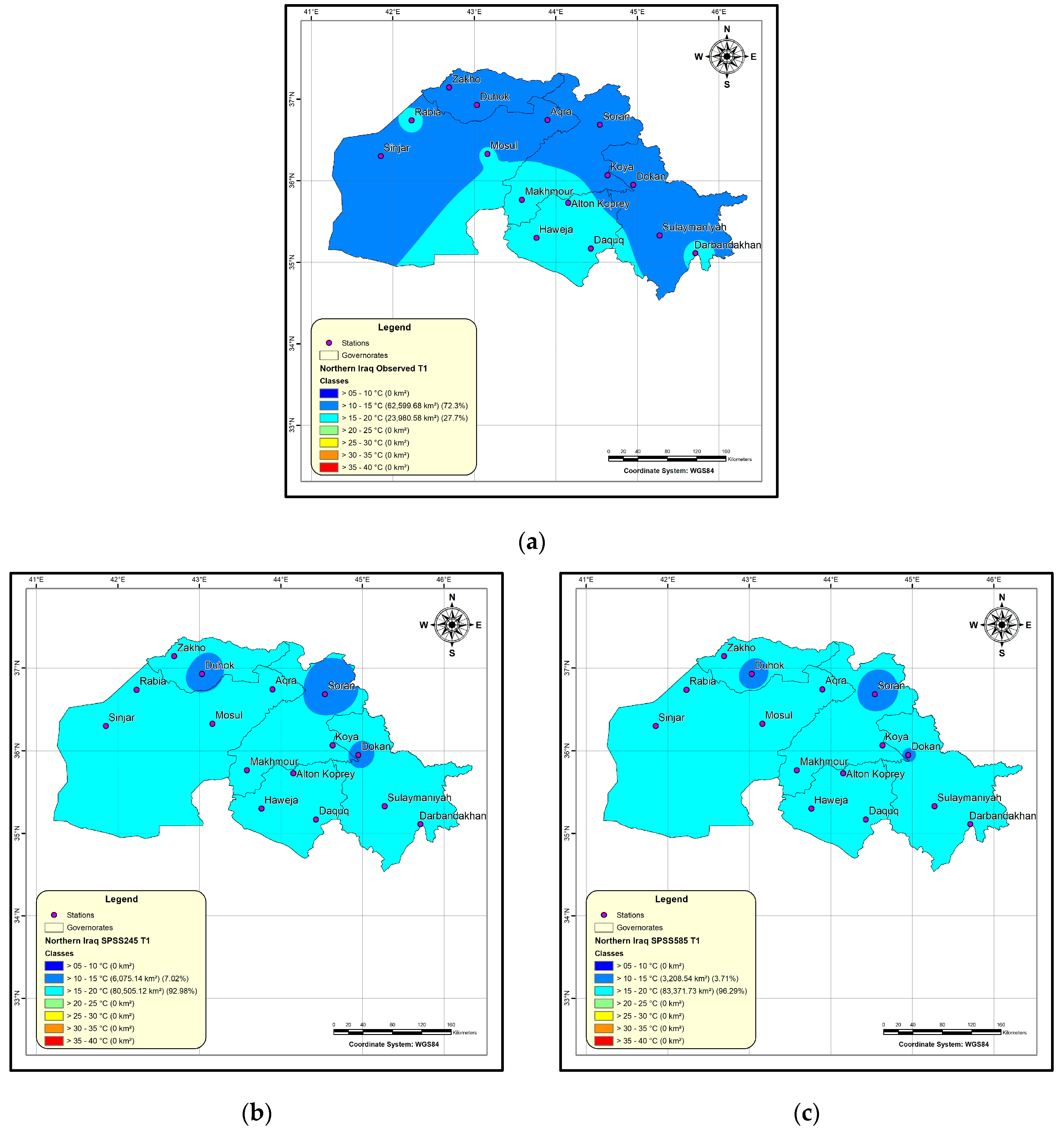
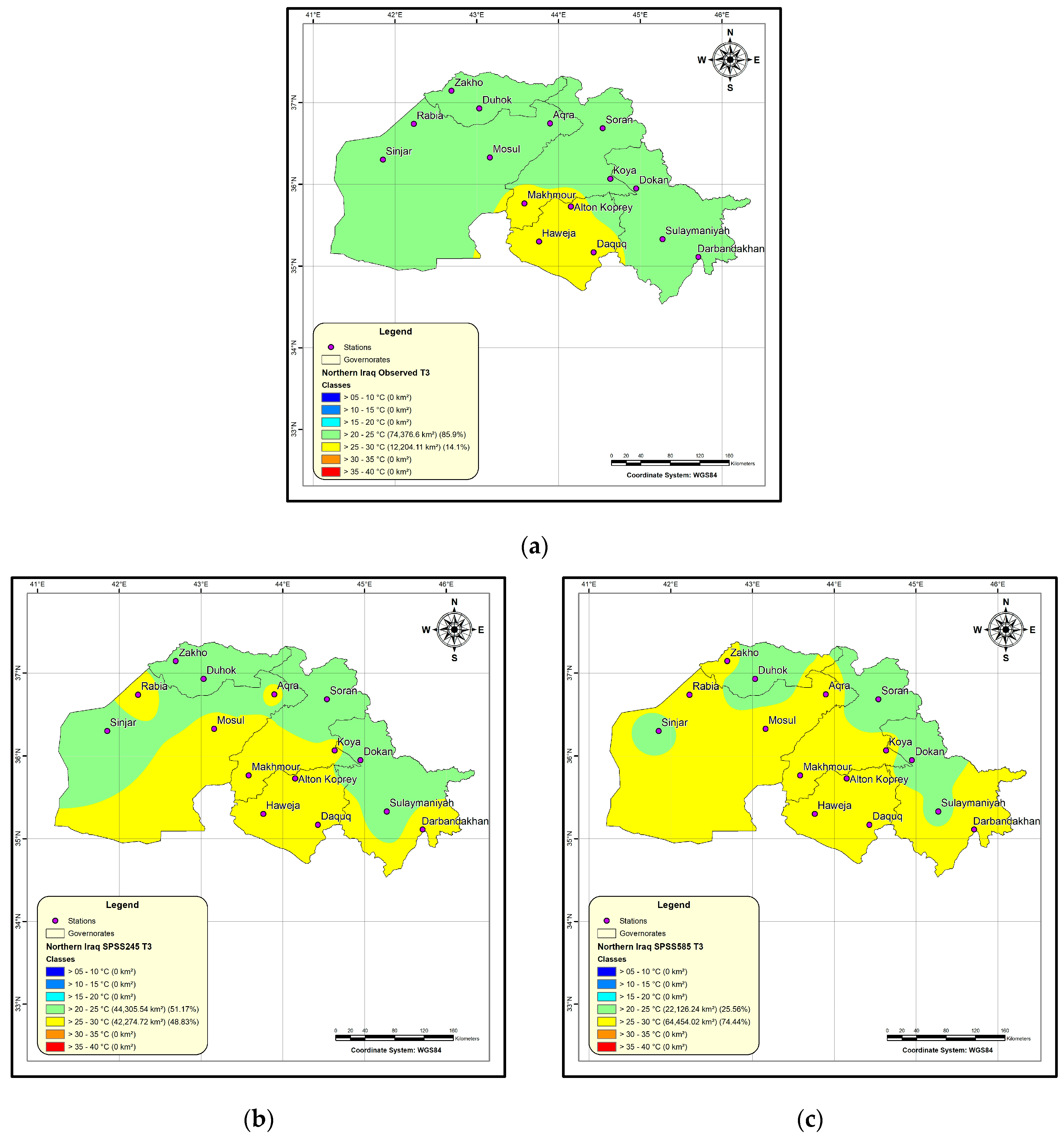
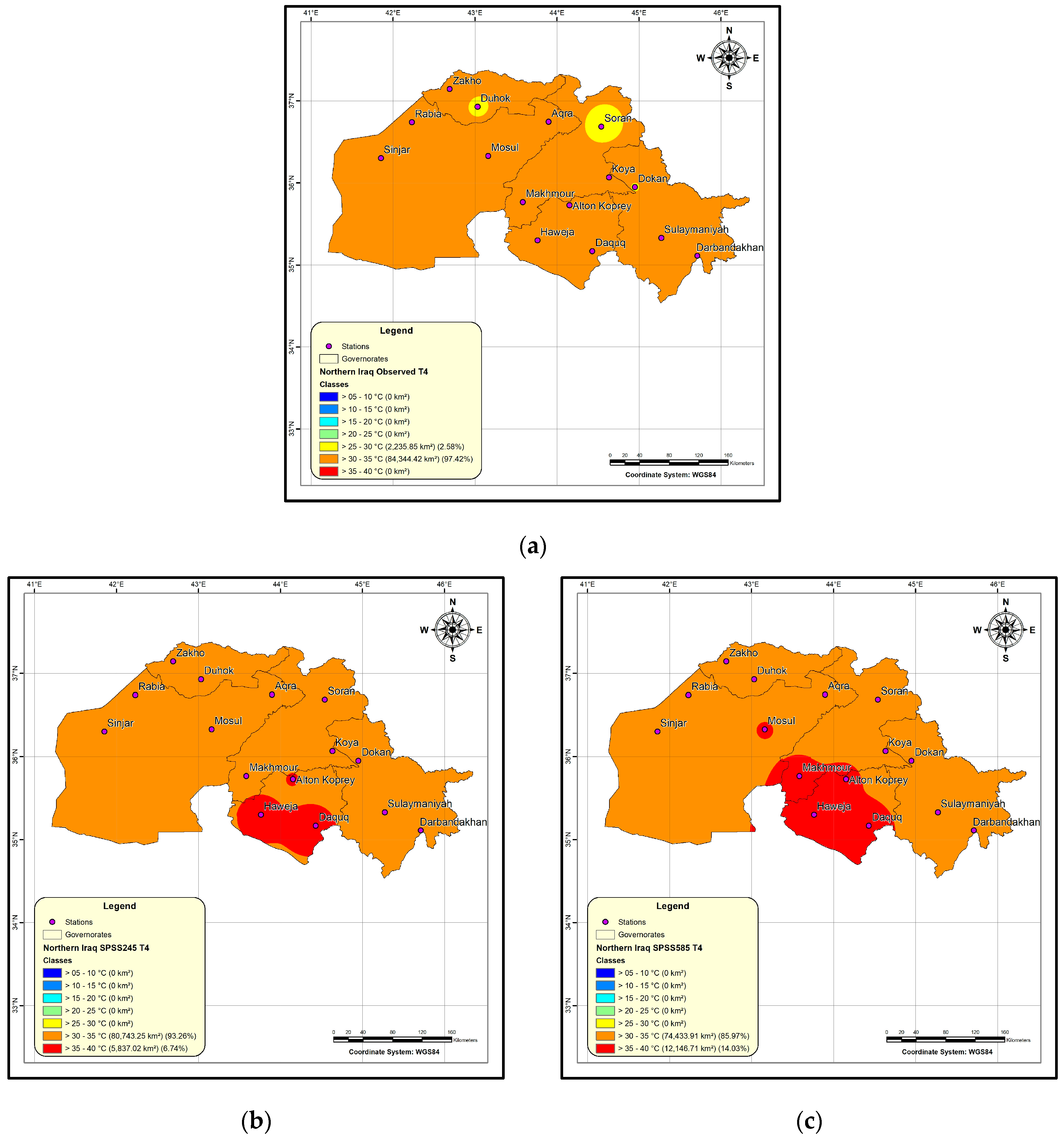
3.2.2. Projection of Mean Temperature
4. Discussion
5. Conclusions
- The LARS-WG (8) model can adequately downscale daily climatic variables for 15 stations based on statistical tests.
- The seasonal spatial-temporal ensemble of five GCMs predicts inconsistent trends in downscaled rainfall across two emission scenarios compared with the historical baseline period. However, it will rise in all seasons except autumn for the SSP585 scenario.
- The highest rainfall increment percentage is obtained using the SSP585 for class (120–140) mm during winter. The spatial extent of the class increased from 25.49 to 50.19%.
- The seasonal spatial-temporal ensemble of five GCMs for mean temperature projected an upward trend across two emission scenarios compared with the historical baseline period. However, the change was generally more noticeable for the SSP585 scenario than for SSP245.
- The highest percentage of increase in mean temperature is achieved using the SSP585 scenario during the autumn season when the spatial coverage of class (15–20) °C increased from 27.7 to 96.29%.
- The alteration pattern of future temperature and precipitation change are spatially compatible. It will be positive for both scenarios throughout the year except for autumn, showing a negative relationship between mean temperature and rainfall under SSP585. Consequently, places receiving more rainfall will witness warmer temperatures.
- A key strength of the present study was that the findings emphasized the value of taking spatial and temporal factors into account since datasets could record drought occurrences at different periods and places, exposing modest differences in the effects of drought. This study has provided a deeper insight into policymakers and managers on managing and planning water resources under climate change’s variability. It impacts the rainfed production and livestock directly when increasing temperature and decreasing rainfall or more frequent flooding and soil erosion when increasing rainfall.
Author Contributions
Funding
Data Availability Statement
Conflicts of Interest
References
- Lee, H.; Calvin, K.; Dasgupta, D.; Krinner, G.; Mukherji, A.; Thorne, P.; Trisos, C.; Romero, J.; Aldunce, P.; Barrett, K. Synthesis Report of the IPCC Sixth Assessment Report (AR6), Longer Report; IPCC: Geneva, Switzerland, 2023; pp. 35–115. [Google Scholar]
- Nile, B.K.; Hassan, W.H.; Alshama, G.A. Analysis of the effect of climate change on rainfall intensity and expected flooding by using ANN and SWMM programs. ARPN J. Eng. Appl. Sci. 2019, 14, 974–984. [Google Scholar]
- Fezzi, C.; Harwood, A.R.; Lovett, A.A.; Bateman, I.J. The environmental impact of climate change adaptation on land use and water quality. Build. A Clim. Resilient Econ. Soc. 2015, 5, 255–260. [Google Scholar] [CrossRef]
- Hinge, G.; Surampalli, R.Y.; Goyal, M.K. Prediction of soil organic carbon stock using digital mapping approach in humid India. Environ. Earth Sci. 2018, 77, 172. [Google Scholar] [CrossRef]
- Pervez, M.S.; Henebry, G.M. Assessing the impacts of climate and land use and land cover change on the freshwater availability in the Brahmaputra River basin. J. Hydrol. Reg. Stud. 2015, 3, 285–311. [Google Scholar] [CrossRef]
- Hassan, W.H.; Hussein, H.; Nile, B.K. The effect of climate change on groundwater recharge in unconfined aquifers in the western desert of Iraq. Groundw. Sustain. Dev. 2022, 16, 100700. [Google Scholar] [CrossRef]
- Hassan, W.H.; Nile, B.K. Climate change and predicting future temperature in Iraq using CanESM2 and HadCM3 modeling. Model. Earth Syst. Environ. 2021, 7, 737–748. [Google Scholar] [CrossRef]
- Nile, B.; Hassan, W.; Esmaeel, B. An evaluation of flood mitigation using a storm water management model [SWMM] in a residential area in Kerbala, Iraq. In IOP Conference Series: Materials Science and Engineering; IOP Publishing: Bristol, UK, 2018; p. 012001. [Google Scholar]
- Usta, D.F.B.; Teymouri, M.; Chatterjee, U.; Koley, B. Temperature projections over Iran during the twenty-first century using CMIP5 models. Model. Earth Syst. Environ. 2021, 8, 749–760. [Google Scholar] [CrossRef]
- Afshar, M.H.; Şorman, A.Ü.; Tosunoğlu, F.; Bulut, B.; Yilmaz, M.T.; Danandeh Mehr, A. Climate change impact assessment on mild and extreme drought events using copulas over Ankara, Turkey. Theor. Appl. Climatol. 2020, 141, 1045–1055. [Google Scholar] [CrossRef]
- Mohammed, S.A.; Fallah, R.Q. Climate change indicators in AlSheikh-Badr basin (Syria). Geogr. Environ. Sustain. 2019, 12, 87–96. [Google Scholar] [CrossRef]
- Hassan, W.H.; Hashim, F.S. The effect of climate change on the maximum temperature in Southwest Iraq using HadCM3 and CanESM2 modelling. SN Appl. Sci. 2020, 2, 1494. [Google Scholar] [CrossRef]
- Tarawneh, Q.Y.; Chowdhury, S. Trends of climate change in Saudi Arabia: Implications on water resources. Climate 2018, 6, 8. [Google Scholar] [CrossRef]
- Knutti, R.; Masson, D.; Gettelman, A. Climate model genealogy: Generation CMIP5 and how we got there. Geophys. Res. Lett. 2013, 40, 1194–1199. [Google Scholar] [CrossRef]
- Guo, X.; Huang, J.; Luo, Y.; Zhao, Z.; Xu, Y. Projection of heat waves over China for eight different global warming targets using 12 CMIP5 models. Theor. Appl. Climatol. 2017, 128, 507–522. [Google Scholar] [CrossRef]
- Xu, L.; Wang, A. Application of the bias correction and spatial downscaling algorithm on the temperature extremes from CMIP5 multimodel ensembles in China. Earth Space Sci. 2019, 6, 2508–2524. [Google Scholar] [CrossRef]
- Sha, J.; Li, X.; Yang, J. Estimation of Watershed Hydrochemical Responses to Future Climate Changes Based on CMIP6 Scenarios in the Tianhe River (China). Sustainability 2021, 13, 102. [Google Scholar] [CrossRef]
- Sayadi, A.; Beydokhti, N.T.; Najarchi, M.; Najafizadeh, M.M. Investigation into the Effects of Climatic Change on Temperature, Rainfall, and Runoff of the Doroudzan Catchment, Iran, Using the Ensemble Approach of CMIP3 Climate Models. Adv. Meteorol. 2019, 2019, 6357912. [Google Scholar] [CrossRef]
- Vallam, P.; Qin, X.S. Projecting future precipitation and temperature at sites with diverse climate through multiple statistical downscaling schemes. Theor. Appl. Climatol. 2017, 134, 669–688. [Google Scholar] [CrossRef]
- Willems, P.; Vrac, M. Statistical precipitation downscaling for small-scale hydrological impact investigations of climate change. J. Hydrol. 2011, 402, 193–205. [Google Scholar] [CrossRef]
- Ahmed, K.F.; Wang, G.; Silander, J.; Wilson, A.M.; Allen, J.M.; Horton, R.; Anyah, R. Statistical downscaling and bias correction of climate model outputs for climate change impact assessment in the U.S. northeast. Glob. Planet. Chang. 2013, 100, 320–332. [Google Scholar] [CrossRef]
- Miralha, L.; Muenich, R.L.; Scavia, D.; Wells, K.; Steiner, A.L.; Kalcic, M.; Apostel, A.; Basile, S.; Kirchhoff, C.J. Bias correction of climate model outputs influences watershed model nutrient load predictions. Sci. Total Environ. 2021, 759, 143039. [Google Scholar] [CrossRef]
- Modi, P.A.; Fuka, D.R.; Easton, Z.M. Impacts of climate change on terrestrial hydrological components and crop water use in the Chesapeake Bay watershed. J. Hydrol. Reg. Stud. 2021, 35, 100830. [Google Scholar] [CrossRef]
- Chen, C.; Gan, R.; Feng, D.; Yang, F.; Zuo, Q. Quantifying the contribution of SWAT modeling and CMIP6 inputting to streamflow prediction uncertainty under climate change. J. Clean. Prod. 2022, 364, 132675. [Google Scholar] [CrossRef]
- Liu, Y.; Chen, X.; Gao, H.; Sha, J.; Li, X. The impacts of climate changes on watershed streamflow and total dissolved nitrogen in Danjiang Watershed, China. J. Water Clim. Chang. 2023, 14, 104–122. [Google Scholar] [CrossRef]
- Rafiei-Sardooi, E.; Azareh, A.; Joorabian Shooshtari, S.; Parteli, E.J.R. Long-term assessment of land-use and climate change on water scarcity in an arid basin in Iran. Ecol. Model. 2022, 467, 109934. [Google Scholar] [CrossRef]
- Mohammadi, E.; Movahedi, S.; Mohammadi, R.; Golkari, S. Assessment of the occurrence of climate change and its effects on planting date and growth duration of rainfed wheat in the western and northwestern regions of Iran. Paddy Water Environ. 2022, 20, 241–253. [Google Scholar] [CrossRef]
- Naderi, M. Extreme climate events under global warming in northern Fars Province, southern Iran. Theor. Appl. Climatol. 2020, 142, 1221–1243. [Google Scholar] [CrossRef]
- Saeed, F.H.; Al-Khafaji, M.S.; Al-Faraj, F.A.M. Sensitivity of Irrigation Water Requirement to Climate Change in Arid and Semi-Arid Regions towards Sustainable Management of Water Resources. Sustainability 2021, 13, 3608. [Google Scholar] [CrossRef]
- Sharma, A.; Sharma, D.; Panda, S.K.; Dubey, S.K.; Pradhan, R.K. Investigation of temperature and its indices under climate change scenarios over different regions of Rajasthan state in India. Glob. Planet. Chang. 2018, 161, 82–96. [Google Scholar] [CrossRef]
- Xu, S.; Wang, K.; Ma, H.; Peng, T.; Li, Y.; Liu, J.; Hu, X.; Su, B.; Dong, X.; Abubakari, S. Modelling streamflow response to climate change in data-scarce White Volta River basin of West Africa using a semi-distributed hydrologic model. J. Water Clim. Chang. 2019, 10, 907–930. [Google Scholar] [CrossRef]
- Birara, H.; Pandey, R.P.; Mishra, S.K. Projections of future rainfall and temperature using statistical downscaling techniques in Tana Basin, Ethiopia. Sustain. Water Resour. Manag. 2020, 6. [Google Scholar] [CrossRef]
- Tibangayuka, N.; Mulungu, D.M.M.; Izdori, F. Assessing the potential impacts of climate change on streamflow in the data-scarce Upper Ruvu River watershed, Tanzania. J. Water Clim. Chang. 2022, 13, 3496–3513. [Google Scholar] [CrossRef]
- Kavwenje, S.; Zhao, L.; Chen, L.; Chaima, E. Projected temperature and precipitation changes using the LARS-WG statistical downscaling model in the Shire River Basin, Malawi. Int. J. Climatol. 2021, 42, 400–415. [Google Scholar] [CrossRef]
- Trnka, M.; Balek, J.; Semenov, M.; Semeradova, D.; Belinova, M.; Hlavinka, P.; Olesen, J.; Eitzinger, J.; Schaumberger, A.; Zahradnicek, P.J.B.P. Future agroclimatic conditions and implications for European grasslands. Biol. Plant. 2021, 64, 865–880. [Google Scholar] [CrossRef]
- Senapati, N.; Griffiths, S.; Hawkesford, M.; Shewry, P.R.; Semenov, M.A. Substantial increase in yield predicted by wheat ideotypes for Europe under future climate. Clim. Res. 2020, 80, 189–201. [Google Scholar] [CrossRef]
- Vesely, F.M.; Paleari, L.; Movedi, E.; Bellocchi, G.; Confalonieri, R. Quantifying Uncertainty Due to Stochastic Weather Generators in Climate Change Impact Studies. Sci. Rep. 2019, 9, 9258. [Google Scholar] [CrossRef]
- Musayev, S.; Burgess, E.; Mellor, J. A global performance assessment of rainwater harvesting under climate change. Resour. Conserv. Recycl. 2018, 132, 62–70. [Google Scholar] [CrossRef]
- Shaygan, M.; Reading, L.P.; Arnold, S.; Baumgartl, T. Modeling the effect of soil physical amendments on reclamation and revegetation success of a saline-sodic soil in a semi-arid environment. Arid Land Res. Manag. 2018, 32, 379–406. [Google Scholar] [CrossRef]
- Alam, M.S.; Barbour, S.L.; Elshorbagy, A.; Huang, M. The Impact of Climate Change on the Water Balance of Oil Sands Reclamation Covers and Natural Soil Profiles. J. Hydrometeorol. 2018, 19, 1731–1752. [Google Scholar] [CrossRef]
- Alam, M.S.; Barbour, S.L.; Huang, M.; Li, Y. Using Statistical and Dynamical Downscaling to Assess Climate Change Impacts on Mine Reclamation Cover Water Balances. Mine Water Environ. 2020, 39, 699–715. [Google Scholar] [CrossRef]
- Gitau, M.W.; Mehan, S.; Guo, T. Weather Generator Effectiveness in Capturing Climate Extremes. Environ. Process. 2018, 5, 153–165. [Google Scholar] [CrossRef]
- Zubaidi, S.L.; Kumar, P.; Al-Bugharbee, H.; Ahmed, A.N.; Ridha, H.M.; Mo, K.H.; El-Shafie, A. Developing a hybrid model for accurate short-term water demand prediction under extreme weather conditions: A case study in Melbourne, Australia. Appl. Water Sci. 2023, 13, 184. [Google Scholar] [CrossRef]
- Khairan, H.E.; Zubaidi, S.L.; Raza, S.F.; Hameed, M.; Al-Ansari, N.; Ridha, H.M. Examination of Single- and Hybrid-Based Metaheuristic Algorithms in ANN Reference Evapotranspiration Estimating. Sustainability 2023, 15, 4222. [Google Scholar] [CrossRef]
- Zakaria, S.; Al-Ansari, N.; Knutsson, S.; Ezz-Aldeen, M. Rain water harvesting and supplemental irrigation at Northern Sinjar Mountain, Iraq. J. Purity Util. React. Environ. 2012, 1, 121–141. [Google Scholar]
- Mohammed, R.; Scholz, M. Climate change and water resources in arid regions: Uncertainty of the baseline time period. Theor. Appl. Climatol. 2019, 137, 1365–1376. [Google Scholar] [CrossRef]
- Mohammed, Z.M.; Hassan, W.H. Climate change and the projection of future temperature and precipitation in southern Iraq using a LARS-WG model. Model. Earth Syst. Environ. 2022, 8, 4205–4218. [Google Scholar] [CrossRef]
- Kuglitsch, F.G.; Toreti, A.; Xoplaki, E.; Della-Marta, P.M.; Zerefos, C.S.; Türkeş, M.; Luterbacher, J. Heat wave changes in the eastern Mediterranean since 1960. Geophys. Res. Lett. 2010, 37, 1–5. [Google Scholar] [CrossRef]
- Selek, B.; Demirel Yazici, D.; Aksu, H.; Özdemir, A.D. Seyhan Dam, Turkey, and Climate Change Adaptation Strategies. In Increasing Resilience to Climate Variability and Change; Springer: Berlin/Heidelberg, Germany, 2016; pp. 205–231. [Google Scholar] [CrossRef]
- Ewaid, S.; Abed, S.; Al-Ansari, N. Water Footprint of Wheat in Iraq. Water 2019, 11, 535. [Google Scholar] [CrossRef]
- Awchi, T.A.; Kalyana, M.M. Meteorological drought analysis in northern Iraq using SPI and GIS. Sustain. Water Resour. Manag. 2017, 3, 451–463. [Google Scholar] [CrossRef]
- Ahmad, H.Q.; Kamaruddin, S.A.; Harun, S.B.; Al-Ansari, N.; Shahid, S.; Jasim, R.M. Assessment of Spatiotemporal Variability of Meteorological Droughts in Northern Iraq Using Satellite Rainfall Data. KSCE J. Civ. Eng. 2021, 25, 4481–4493. [Google Scholar] [CrossRef]
- Hashim, B.M.; Al Maliki, A.; Alraheem, E.A.; Al-Janabi, A.M.S.; Halder, B.; Yaseen, Z.M. Temperature and precipitation trend analysis of the Iraq Region under SRES scenarios during the twenty-first century. Theor. Appl. Climatol. 2022, 148, 881–898. [Google Scholar] [CrossRef]
- Kadhim Tayyeh, H.; Mohammed, R. Analysis of NASA POWER reanalysis products to predict temperature and precipitation in Euphrates River basin. J. Hydrol. 2023, 619, 129327. [Google Scholar] [CrossRef]
- Oliazadeh, A.; Bozorg-Haddad, O.; Mani, M.; Chu, X. Developing an urban runoff management model by using satellite precipitation datasets to allocate low impact development systems under climate change conditions. Theor. Appl. Climatol. 2021, 146, 675–687. [Google Scholar] [CrossRef]
- Oviroh, P.O.; Austin-Breneman, J.; Chien, C.-C.; Chakravarthula, P.N.; Harikumar, V.; Shiva, P.; Kimbowa, A.B.; Luntz, J.; Miyingo, E.W.; Papalambros, P.Y. Micro Water-Energy-Food (MicroWEF) Nexus: A system design optimization framework for Integrated Natural Resource Conservation and Development (INRCD) projects at community scale. Appl. Energy 2023, 333, 120583. [Google Scholar] [CrossRef]
- Semenov, M.A.; Brooks, R.J.; Barrow, E.M.; Richardson, C.W. Comparison of the WGEN and LARS-WG stochastic weather generators for diverse climates. Clim. Res. 1998, 10, 95–107. [Google Scholar] [CrossRef]
- Babaeian, I.; Najafi, Z. Climate change assessment in Khorasan-e Razavi Province from 2010 to 2039 using statistical downscaling of GCM Output. J. Geogr. Reg. 2010, 8. [Google Scholar] [CrossRef]
- Semenov, M.A.; Barrow, E.M. Lars-Wg A Stochastic Weather Generator for Use in Climate Impact Studies. 2002, pp. 1–27. Available online: https://www.researchgate.net/publication/268304865_LARS-WG_A_Stochastic_Weather_Generator_for_Use_in_Climate_Impact_Studies (accessed on 29 January 2024).
- Semenov, M.A.; Pilkington-Bennett, S.; Calanca, P. Validation of ELPIS 1980–2010 baseline scenarios using the observed European Climate Assessment data set. Clim. Res. 2013, 57, 1–9. [Google Scholar] [CrossRef]
- Chen, H.; Guo, J.; Zhang, Z.; Xu, C.-Y. Prediction of temperature and precipitation in Sudan and South Sudan by using LARS-WG in future. Theor. Appl. Climatol. 2013, 113, 363–375. [Google Scholar] [CrossRef]
- Venkataraman, K.; Tummuri, S.; Medina, A.; Perry, J. 21st century drought outlook for major climate divisions of Texas based on CMIP5 multimodel ensemble: Implications for water resource management. J. Hydrol. 2016, 534, 300–316. [Google Scholar] [CrossRef]
- Ishaque, W.; Osman, R.; Hafiza, B.S.; Malghani, S.; Zhao, B.; Xu, M.; Ata-Ul-Karim, S.T. Quantifying the impacts of climate change on wheat phenology, yield, and evapotranspiration under irrigated and rainfed conditions. Agric. Water Manag. 2023, 275, 108017. [Google Scholar] [CrossRef]
- Tebaldi, C.; Knutti, R. The use of the multi-model ensemble in probabilistic climate projections. Philos. Trans. R. Soc. A Math. Phys. Eng. Sci. 2007, 365, 2053–2075. [Google Scholar] [CrossRef]
- Weiland, F.S.; Van Beek, L.; Weerts, A.; Bierkens, M. Extracting information from an ensemble of GCMs to reliably assess future global runoff change. J. Hydrol. 2012, 412, 66–75. [Google Scholar] [CrossRef]
- Zhai, P.; Zhou, B.; Chen, Y. A Review of Climate Change Attribution Studies. J. Meteorol. Res. 2018, 32, 671–692. [Google Scholar] [CrossRef]
- Kolyvas, C.; Missiakoulis, S.; Gofa, F. Mean Daily Temperature Estimations and the Impact on Climatological Applications. In Proceedings of the 16th International Conference on Meteorology, Climatology and Atmospheric Physics—COMECAP 2023, Athens, Greece, 25–29 September 2023. [Google Scholar]
- Khalaf, R.M.; Hussein, H.H.; Hassan, W.H.; Mohammed, Z.M.; Nile, B.K. Projections of precipitation and temperature in Southern Iraq using a LARS-WG Stochastic weather generator. Phys. Chem. Earth Parts A/B/C 2022, 128. [Google Scholar] [CrossRef]
- Munawar, S.; Rahman, G.; Moazzam, M.F.U.; Miandad, M.; Ullah, K.; Al-Ansari, N.; Linh, N.T.T. Future Climate Projections Using SDSM and LARS-WG Downscaling Methods for CMIP5 GCMs over the Transboundary Jhelum River Basin of the Himalayas Region. Atmosphere 2022, 13, 898. [Google Scholar] [CrossRef]
- Zamani, M.G.; Saniei, K.; Nematollahi, B.; Zahmatkesh, Z.; Moghadari Poor, M.; Nikoo, M.R. Developing sustainable strategies by LID optimization in response to annual climate change impacts. J. Clean. Prod. 2023, 416. [Google Scholar] [CrossRef]
- Sheikhbabaei, A.; Hosseini Baghanam, A.; Zarghami, M.; Pouri, S.; Hassanzadeh, E. System Thinking Approach toward Reclamation of Regional Water Management under Changing Climate Conditions. Sustainability 2022, 14, 9411. [Google Scholar] [CrossRef]
- Alasow, A.A.; Hamed, M.M.; Shahid, S. Spatiotemporal variability of drought and affected croplands in the horn of Africa. Stoch. Environ. Res. Risk Assess. 2023, 38, 281–296. [Google Scholar] [CrossRef]
- Merabti, A.; Martins, D.S.; Meddi, M.; Pereira, L.S. Spatial and Time Variability of Drought Based on SPI and RDI with Various Time Scales. Water Resour. Manag. 2017, 32, 1087–1100. [Google Scholar] [CrossRef]
- Muhire, I.; Tesfamichael, S.G.; Ahmed, F.; Minani, E. Spatio-temporal trend analysis of projected precipitation data over Rwanda. Theor. Appl. Climatol. 2016, 131, 671–680. [Google Scholar] [CrossRef]
- Bayatavrkeshi, M.; Imteaz, M.A.; Kisi, O.; Farahani, M.; Ghabaei, M.; Al-Janabi, A.M.S.; Hashim, B.M.; Al-Ramadan, B.; Yaseen, Z.M. Drought trends projection under future climate change scenarios for Iran region. PLoS ONE 2023, 18, e0290698. [Google Scholar] [CrossRef]
- Bahrami, M.; Bazrkar, S.; Zarei, A.R. Spatiotemporal investigation of drought pattern in Iran via statistical analysis and GIS technique. Theor. Appl. Climatol. 2020, 143, 1113–1128. [Google Scholar] [CrossRef]
- Motiee, H.; McBean, E.; Motiee, A.R.; Majdzadeh Tabatabaei, M.R. Assessment of climate change under CMIP5-RCP scenarios on downstream rivers glaciers–Sardabrud River of Alam-Kuh glacier, Iran. Int. J. River Basin Manag. 2020, 18, 39–47. [Google Scholar] [CrossRef]
- Khan, S.F.; Naeem, U.A. Future climate projections using the LARS-WG6 downscaling model over Upper Indus Basin, Pakistan. Environ. Monit Assess 2023, 195, 810. [Google Scholar] [CrossRef] [PubMed]
- Babaeian, E.; Nagafineik, Z.; Zabolabasi, F.; Habeibei, M.; Adab, H.; Malbisei, S. Climate change assessment over Iran during 2010-2039 by using statistical downscaling of ECHO-G model. Geogr. Dev. 2009, 7, 135–152. [Google Scholar] [CrossRef]
- Groisman, P.Y.; Bradley, R.S.; Bomin, S. The Relationship of Cloud Cover to Near-Surface Temperature and Humidity:Comparison of GCM Simulations with Empirical Data. Climate 2000, 13, 1858–1878. [Google Scholar] [CrossRef]
- Zhong, X.; Liu, S.C.; Liu, R.; Wang, X.; Mo, J.; Li, Y. Observed trends in clouds and precipitation (1983–2009): Implications for their cause(s). Atmos. Chem. Phys. 2021, 21, 4899–4913. [Google Scholar] [CrossRef]
- Seneviratne, S.I.; Zhang, X.; Adnan, M.; Badi, W.; Dereczynski, C.; Luca, A.D. Weather and Climate Extreme Events in a Changing Climate. In Climate Change 2021—The Physical Science Basis; Cambridge University Press: Cambridge, UK, 2023; pp. 1513–1766. [Google Scholar] [CrossRef]
- Hadi, S.J.; Tombul, M. Comparison of Spatial Interpolation Methods of Precipitation and Temperature Using Multiple Integration Periods. J. Indian Soc. Remote Sens. 2018, 46, 1187–1199. [Google Scholar] [CrossRef]
- Shope, C.L.; Maharjan, G.R. Modeling Spatiotemporal Precipitation: Effects of Density, Interpolation, and Land Use Distribution. Adv. Meteorol. 2015, 2015, 174196. [Google Scholar] [CrossRef]
- Li, J.; Heap, A.D. Spatial interpolation methods applied in the environmental sciences: A review. Environ. Model. Softw. 2014, 53, 173–189. [Google Scholar] [CrossRef]


| Province | Station | Longitude | Latitude | Elevation |
|---|---|---|---|---|
| Duhok | Duhok | 43.03 | 36.93 | 569 |
| Aqra | 43.90 | 36.75 | 636 | |
| Zakho | 42.69 | 37.14 | 444 | |
| Erbel | Makhmour | 43.58 | 35.77 | 261 |
| Soran | 44.54 | 36.69 | 728 | |
| Koya | 44.63 | 36.07 | 557 | |
| Sulaymaniyah | Sulaymaniyah City | 45.27 | 35.33 | 885 |
| Darbandikhan Dam | 45.71 | 35.11 | 610 | |
| Dokan Dam | 44.95 | 35.95 | 489 | |
| Mosul | Mosul City | 43.16 | 36.33 | 238 |
| Sinjar | 41.85 | 36.30 | 517 | |
| Rabia | 42.23 | 36.74 | 368 | |
| Kirkuk | Daquq | 44.43 | 35.17 | 227 |
| Alton Koprey | 44.15 | 35.73 | 261 | |
| Haweja | 43.76 | 35.30 | 184 |
| Stations | Tmin | Tmax | Rainfall | ||||||
|---|---|---|---|---|---|---|---|---|---|
| Max. | Min. | Mean | Max. | Min. | Mean | Max. | Min. | Mean | |
| Duhok | 25.55 | −4.274 | 10.914 | 42.102 | 3.37 | 22.914 | 122.67 | 0 | 28.987 |
| Aqra | 28.382 | −1.879 | 13.287 | 45.660 | 7.497 | 27.024 | 153.58 | 0 | 26.373 |
| Zakho | 28.624 | −1.408 | 13.634 | 45.208 | 6.555 | 26.165 | 148.24 | 0 | 28.879 |
| Makhmour | 28.987 | −1.195 | 14.176 | 46.350 | 8.922 | 27.967 | 129.46 | 0 | 20.820 |
| Soran | 24.518 | −4.757 | 9.8556 | 41.965 | 4.476 | 23.518 | 168.61 | 0 | 24.278 |
| Koya | 27.903 | −1.833 | 13.106 | 45.121 | 7.014 | 26.607 | 139.98 | 0 | 22.598 |
| Sulaymaniyah | 26.493 | −2.519 | 12.165 | 43.860 | 6.621 | 25.873 | 135.43 | 0 | 23.109 |
| Darbandikhan | 26.778 | −1.807 | 12.869 | 44.843 | 8.441 | 27.328 | 121.7 | 0 | 22.537 |
| Dokan | 25.505 | −3.597 | 11.284 | 42.465 | 4.682 | 24.133 | 142.77 | 0 | 23.939 |
| Mosul | 29.253 | −1.620 | 13.542 | 45.934 | 7.721 | 27.203 | 124.34 | 0 | 24.003 |
| Sinjar | 27.006 | −2.367 | 12.462 | 44.047 | 7.268 | 25.952 | 119.21 | 0 | 20.512 |
| Rabia | 28.776 | −1.740 | 13.598 | 45.587 | 7.809 | 27.097 | 125.01 | 0 | 22.332 |
| Daquq | 30.160 | −0.127 | 15.639 | 47.09 | 10.862 | 29.558 | 115.9 | 0 | 18.070 |
| Alton Koprey | 29.008 | −0.954 | 14.396 | 46.228 | 9.145 | 28.225 | 124.44 | 0 | 20.198 |
| Haweja | 29.599 | −0.765 | 14.775 | 46.787 | 10.100 | 28.923 | 119.31 | 0 | 16.303 |
| No. | GCM Models | Institution/Country | Spatial Resolution |
|---|---|---|---|
| 1 | ACCESS-ESM1-5 | Australian Community Climate and Earth System Simulator, Acton, Australia | 192 × 144 |
| 2 | CNRM-CM6-1 | Centre National de Recherches Météorologiques, Toulouse, France | 256 × 128 |
| 3 | HadGEM3-GC31-LL | Met Office, United Kingdom | 192 × 144 |
| 4 | MPI-ESM1-2-LR | Max Planck Institute, Hamburg, Germany | 192 × 96 |
| 5 | MRI-ESM2-0 | Meteorological Research Institute, Tsukuba, Japan | 320 × 160 |
| No. | SSP | Description |
|---|---|---|
| 1 | SSP2-4.5 | Moderate GHG emissions: CO2 emissions will remain at current levels until 2050, after which they will decline but not completely disappear by 2100. |
| 2 | SSP5-8.5 | Extremely high GHG emissions: by 2075, CO2 emissions will quadruple. 2.4 °C 4.4 °C 3.3–5.7 GHG: Greenhouse gas. |
| A. K-S Test for Distributions of the Seasonal Wet and Dry Series. | |||||
| Season | Wet/Dry | N | K-S | p-Value | Assessment |
| Dec., Jan., and Feb. | Wet | “11.5” | 0.080 | 1.000 | P |
| Dry | 11.5 | 0.084 | 1.000 | P | |
| Mar., Apr., and May | Wet | 11.5 | 0.059 | 0.984 | V G |
| Dry | 11.5 | 0.130 | 1.000 | P | |
| Jun., Jul., and Aug. | Wet | 11.5 | 0.079 | 1.000 | P |
| Dry | 11.5 | 0.070 | 1.000 | P | |
| Sep., Oct., and Nov. | Wet | 11.5 | 0.059 | 1.000 | P |
| Dry | 11.5 | 0.065 | 1.000 | P | |
| B. K-S-Test for Distributions of Daily Rainfall. | |||||
| Month | N | K-S | p-Value | Assessment | |
| Jan. | 11.5 | 0.065 | 1.000 | P | |
| Feb. | 11.5 | 0.050 | 1.000 | P | |
| Mar. | 11.5 | 0.028 | 1.000 | P | |
| Apr. | 11.5 | 0.045 | 1.000 | P | |
| May | 11.5 | 0.030 | 1.000 | P | |
| Jun. | 11.5 | 0.030 | 1.000 | P | |
| Jul. | 11.5 | 0.025 | 1.000 | P | |
| Aug. | 11.5 | 0.031 | 1.000 | P | |
| Sep. | 11.5 | 0.048 | 1.000 | P | |
| Oct. | 11.5 | 0.060 | 1.000 | P | |
| Nov. | 11.5 | 0.037 | 1.000 | P | |
| Dec. | 11.5 | 0.082 | 1.000 | P | |
| C. KS-Test for Daily MIN Distributions. | |||||
| Month | N | K-S | p-Value | Assessment | |
| Jan. | 11.5 | 0.053 | 1.000 | P | |
| Feb. | 11.5 | 0.053 | 1.000 | P | |
| Mar. | 11.5 | 0.053 | 1.000 | P | |
| Apr. | 11.5 | 0.053 | 1.000 | P | |
| May | 11.5 | 0.053 | 1.000 | P | |
| Jun. | 11.5 | 0.053 | 1.000 | P | |
| Jul. | 11.5 | 0.053 | 1.000 | P | |
| Aug. | 11.5 | 0.053 | 1.000 | P | |
| Sep. | 11.5 | 0.053 | 1.000 | P | |
| Oct. | 11.5 | 0.053 | 1.000 | P | |
| Nov. | 11.5 | 0.053 | 1.000 | P | |
| Dec. | 11.5 | 0.053 | 1.000 | P | |
| D. KS-Test for Daily MAX Distributions. | |||||
| Month | N | K-S | p-Value | Assessment | |
| Jan. | 11.5 | 0.053 | 1.000 | P | |
| Feb. | 11.5 | 0.053 | 1.000 | P | |
| Mar. | 11.5 | 0.053 | 1.000 | P | |
| Apr. | 11.5 | 0.053 | 1.000 | P | |
| May | 11.5 | 0.053 | 1.000 | P | |
| Jun. | 11.5 | 0.053 | 1.000 | P | |
| Jul. | 11.5 | 0.053 | 1.000 | P | |
| Aug. | 11.5 | 0.105 | 0.999 | V G | |
| Sep. | 11.5 | 0.053 | 1.000 | P | |
| Oct. | 11.5 | 0.053 | 1.000 | P | |
| Nov. | 11.5 | 0.053 | 1.000 | P | |
| Dec. | 11.5 | 0.105 | 0.999 | V G | |
| Climate Factors | R | RMSE (°C) | MAE (°C) | MBE (°C) |
| Maximum temperature | 0.99 | 1.8371 | 1.4038 | 0.0145 |
| Minimum temperature | 0.99 | 1.4926 | 1.1478 | −0.0062 |
| Climate Factors | R | RMSE (mm) | MAE (mm) | MBE (mm) |
| Rainfall | 0.74 | 29.2591 | 19.3259 | 0.6725 |
Disclaimer/Publisher’s Note: The statements, opinions and data contained in all publications are solely those of the individual author(s) and contributor(s) and not of MDPI and/or the editor(s). MDPI and/or the editor(s) disclaim responsibility for any injury to people or property resulting from any ideas, methods, instructions or products referred to in the content. |
© 2024 by the authors. Licensee MDPI, Basel, Switzerland. This article is an open access article distributed under the terms and conditions of the Creative Commons Attribution (CC BY) license (https://creativecommons.org/licenses/by/4.0/).
Share and Cite
Abdulsahib, S.M.; Zubaidi, S.L.; Almamalachy, Y.; Dulaimi, A. Temperature and Precipitation Change Assessment in the North of Iraq Using LARS-WG and CMIP6 Models. Water 2024, 16, 2869. https://doi.org/10.3390/w16192869
Abdulsahib SM, Zubaidi SL, Almamalachy Y, Dulaimi A. Temperature and Precipitation Change Assessment in the North of Iraq Using LARS-WG and CMIP6 Models. Water. 2024; 16(19):2869. https://doi.org/10.3390/w16192869
Chicago/Turabian StyleAbdulsahib, Sura Mohammed, Salah L. Zubaidi, Yousif Almamalachy, and Anmar Dulaimi. 2024. "Temperature and Precipitation Change Assessment in the North of Iraq Using LARS-WG and CMIP6 Models" Water 16, no. 19: 2869. https://doi.org/10.3390/w16192869
APA StyleAbdulsahib, S. M., Zubaidi, S. L., Almamalachy, Y., & Dulaimi, A. (2024). Temperature and Precipitation Change Assessment in the North of Iraq Using LARS-WG and CMIP6 Models. Water, 16(19), 2869. https://doi.org/10.3390/w16192869