Subgrid Model of Water Storage in Paddy Fields for a Grid-Based Distributed Rainfall–Runoff Model and Assessment of Paddy Field Dam Effects on Flood Control

Abstract

Paddy field dams are basin-level flood control measures that promote rainwater storage; however, a general runoff model cannot adequately describe the water balance in paddy fields. This study develops a subgrid model for evaluating paddy water balance considering land use on a computational grid. Subgrid models can account for the storage effect of paddy field dams without disregarding the general grid-based distributed rainfall–runoff model framework. To investigate the effect of current paddy field storage and the introduction of paddy field dams on reducing peak flood discharge, rainfall–runoff analysis was conducted using the proposed model in the Kashima River basin, which flows into Lake Inba-numa in Chiba Prefecture, Japan. The computational results indicated that the rainwater storage effect of current paddy fields reduces the peak river discharge, suggesting that the drainage process of the paddy field should be incorporated into runoff models. Furthermore, the storage effect of paddy fields became more pronounced as the height of the drainage pipe in the paddy field dam increased. The calculated results quantitatively show the flood control effect of paddy field storage over the entire basin; thus, the proposed subgrid model may be a useful tool for promoting basin-level flood control measures.

1. Introduction

In recent years, numerous large-scale heavy rainfall disasters have been reported worldwide. In 2020, severe flooding occurred in Indonesia [1] and the Yangtze River in China [2]. In 2021, extreme precipitation and flooding events took place in Germany, Belgium, and The Netherlands [3]. In Japan, Western Japan, the heavy rain of 2018, Typhoon Hagibis in 2019, and the heavy rainfall in July 2020 had significant adverse effects on the population and caused economic losses [4,5,6], with the events in 2018 and 2019 increasing the total rainfall by 6.7% and 10.9%, respectively [7,8]. The Intergovernmental Panel on Climate Change Sixth Assessment Report (IPCC AR6) showed that anthropogenic activities have led to the warming of the atmosphere, ocean, and land and revealed that human-induced climate change is exacerbating weather extremes globally, such as heavy precipitation [9]. Such conditions require the development and implementation of flood control measures to address the increasing precipitation driven by climate change.

Common flood control measures include river improvements, such as levee construction, channel widening, excavation, and tree felling, as well as the construction of dams and flood control reservoirs. In addition to these flood control measures, the promotion of basin-wide flood control measures and damage mitigation measures for evacuation and housing protection is essential to address recent heavy rainfall disasters. The Ministry of Land Infrastructure, Transport and Tourism (MLIT) in Japan established the River Basin Disaster Resilience and Sustainability by All (RBDRSA) policy on water-related disaster risk reduction [10]. This policy covers flood prevention, exposure reduction, and disaster resilience. All the stakeholders in the basin, including residents and businesses, are expected to jointly address these issues. In addition to conventional river maintenance, various hard and soft measures such as rainwater harvesting and infiltration facilities, the advanced release of water from irrigation dams, paddy field storage, land use regulation, and early evacuation are included in this policy. Developing a method for quantitatively evaluating the effects of flood control measures is essential for promoting this policy and improving comprehension and cooperation among stakeholders.

Paddy field storage is a common flood control measure detailed in this policy and has drawn significant attention. Studies focusing on the storage effect of paddy fields and their range of functions [11,12] have been conducted in Taiwan [13,14], Japan [15,16], Korea [17,18], Indonesia [19], and China [20]. Extensive research has also been performed on paddy field dams, which promote the storage effect of paddy fields [21]. Yoshikawa et al. [21] conducted a runoff analysis in Kamigayashi District, Niigata Prefecture, Japan, and found that the construction of a paddy field dam contributes to reducing the peak river discharge and water level, providing flood control in the downstream area. Miyazu et al. [22] investigated the effects and limitations of introducing paddy field dams under various rainfall conditions and showed that the maximum effect for paddy field dams can be achieved with a 120-year rainfall probability (=268 mm/day). Based on runoff analysis, Kobayashi et al. [23] reported that the effects of paddy field dams on reducing the peak discharge in downstream rivers vary according to rainfall conditions. Paddy field dams are also being used outside Japan. For instance, Chen et al. [24] investigated the effects of different drainage mechanisms from paddy fields on runoff in Taiwan using experiments and numerical analyses. However, in these previous studies, field experiments and numerical calculations on paddy field dams were predominantly conducted in small basins, and verification of the effects on the entire basin has been limited [25].

Physically based, grid-based, and distributed rainfall–runoff models can reflect the spatial distribution of the topography and land use conditions within the basin. Therefore, these models are useful for the quantitative evaluation of basin flood control measures, including paddy field storage [26,27,28,29,30,31]. Numerous studies have analyzed land use using the distributed rainfall–runoff model, including paddy field use [25,28,32]; however, one land use type is generally given for each grid. Therefore, the area for each land cover type is not accurately reflected, and this deviation is more pronounced for coarser grids [33]. The process of rainwater drainage from the outlet of a paddy field surrounded by banks differs from that of other land uses; however, these processes are not generally considered in runoff models.

There are two possible solutions to these issues: introduce a subgrid model that can be used to examine the information in the grid and perform individual analyses of each paddy field. Subgrid models have been proposed for the analysis of factors such as topography, land cover, and soil properties [34,35,36,37,38]. However, none of the currently available subgrid models adequately account for water balance processes in paddy fields. In contrast, an individual analysis of each paddy field has been widely applied in runoff analysis to determine the effectiveness of paddy field dams [21,22,23]. These analyses have predominantly been performed in small basins, and their application at the entire basin level does not generate realistic results owing to the complexity of individual analyses. Using the grid-based model, Jung et al. [39] modeled the runoff from a paddy field mesh using a roughness coefficient to account for the water balance in the paddy field. However, precisely adjusting the drainage volume according to the conditions of a paddy field dam is difficult. Chai et al. [25] obtained the discharge from a paddy field mesh and applied it to the adjacent mesh to determine the water balance in a paddy field; however, the land use type for each grid was given, and the treatment of the paddy field depended on the grid resolution. This necessitates the development of a subgrid model that is easily applicable in grid-based distributed rainfall–runoff models to appropriately account for the water balance processes in the paddy field.

This study aimed to develop a subgrid model for paddy field storage that could be incorporated into a grid-based, distributed rainfall–runoff model for the quantitative evaluation of flood control measures based on RBDRSA throughout a basin. The subgrid model was then incorporated into a distributed rainfall–runoff–inundation (RRI) model [30,40]. Using this model, the effects of the current paddy storage and the introduction of paddy field dams on the reduction in river flood discharge were examined in the Kashima River basin, which drains into Lake Inba-numa in Chiba Prefecture, Japan. This study focused on Typhoon Bualoi in 2019 because it caused extensive flood inundation in the Kashima River basin. In this simulation, we set up a paddy field dam model focusing on the outlet, which was composed of circular pipes. This subgrid model may help quantitatively evaluate the effects of current paddy storage and paddy field dams introduced as a flood control measure at the basin level.

2. Study Site

Figure 1 shows the elevation contours and land use map of the Kashima River basin, which is one of the largest inflow rivers of Lake Inba-numa. Lake Inba-numa forms part of the Tone River system and is one of the most eutrophic lakes in Japan. It is divided into the following two parts: the north lake and the west lake. The spatial area of the lake is 11.55 km², the volume is 19.70 million m³, and the average depth is 1.7 m. This shallow lake provides drinking, industrial, and agricultural water. The basin area is 541.1 km², and the population of the basin is 780,000. Kashima River originates from Showa-no-mori Park in Chiba City at an elevation of approximately 95 m. It flows northeastward, merges with the Takasaki River (the largest tributary river), and flows into the west lake (Figure 1b). Kashima River covers an area of 250.4 km², which is 46% of the total area of the Lake Inba-numa basin, 86.7 km² of which is covered by the Takasaki River. The main channel lengths for the Kashima and Takasaki Rivers are 31.8 km and 12.2 km, respectively. The topographical features of the river basin comprise a plateau and valley-like wetlands, known as “yatsu”, where a portion of the plateau is eroded.

According to the high-resolution land use map (approximately 10 m; Japan Aerospace Exploration Agency, JAXA), farmlands (43.0%) are the most common land use type in the Kashima River basin (Figure 1c) and are distributed on the plateau of the Kashima River and the upper reaches of Takasaki River. Forests and urban areas account for 28.6% and 20.7% of the total basin area, respectively. Paddy fields occupy 7.5% of the basin area and are distributed along the rivers. This value is almost the same as the average value for the spatial area of paddy fields in Japan (approximately 9%, [41]). We examined the drainage methods for 174 paddy fields in Kashima River basin. The drainage methods were classified into the following three types: free-draining pipes, drainage boxes, and notches (Figure 2a). Of the 174 paddy fields surveyed, 83.5%, 11.4%, and 5.1% used free-draining pipes, drainage boxes, and notches, respectively. The average height of the pipe bottom from the bed of the paddy field and the diameter of the free-draining pipes were 0.022 m and 0.10 m, respectively (Figure 2b). The mean height of the paddy field banks was 0.24 m. These values were used in the runoff simulation for the current condition of paddy fields.

Heavy rainfall has frequently occurred in the Kashima River basin in recent years. On 25 October 2019, a low-pressure system along the south coast of Japan and Typhoon Bualoi caused heavy rainfall, predominantly on the Pacific side of the Kanto and Tohoku regions. The heavy rainfall caused severe floods that led to significant damage in Chiba Prefecture, especially in the Kashima River basin, where an average of 260 mm of daily rainfall was recorded (Figure S1). This caused overflow flooding from the Kashima and Takasaki Rivers [42], which inundated an area of at least 6.1 km² at an average depth of 1.17 m. Paddy fields in the lowlands along the rivers accounted for most of the flooded area.

3. Methods

3.1. Modeling Methods

3.1.1. Subgrid Model for Water Storage in Paddy Fields

In this study, to overcome the limitations of the existing runoff models, we developed a subgrid model that could be used to evaluate the paddy water balance while considering the land use distribution in the computational grid. As shown in Figure 3, the fundamental concept of the model is to maintain the general grid-based distributed rainfall–runoff model framework, reflect fine-scale land use variation in the computational grid, and examine the storage effect of the paddy field in addressing water balance in the computational grid for paddy fields and non-paddies, respectively. To facilitate the implementation of the subgrid model in the existing distributed rainfall–runoff model, we constructed a grid-based-distributed rainfall–runoff model without making substantial changes in the basic equations and the calculation code (Figure 3a). In the RRI model used in this study, the computational grid is divided into slopes and river channels [43]. The slope grids correspond to the land grids. The equations of continuity and motion based on the diffusion wave approximation for planar two- and one-dimensional fields are applied for slopes and river channels, respectively [30]. We considered land use change at a smaller scale than the computational grid (Figure 3b). Land use was aggregated into the following four categories: paddy fields, farmlands, forests, and impervious areas (such as urban areas). The area fraction for each land use α_i is calculated for each grid, with subscripts i = 1, 2, 3, and 4 corresponding to paddy fields, farmlands, forests, and urban areas, respectively. The infiltration capacity and roughness of each land use were also considered. The land use was divided into paddy fields and non-paddy fields, and the water balance for the paddy field area was calculated by considering the storage and drainage of the paddy field surrounded by the banks (Figure 3c). The drainage water from the paddy field was assumed to be input into the non-paddy section of the same grid. In the non-paddy section, the amount of drainage from the paddy field was considered. For the remainder of the model, the previously used water balance calculations were applied in the slope grid. Although the basic form of the RRI model did not change, the calculation procedure for the slope grid was partially modified to accommodate the land use in the subgrid scale and reflect the water balance unique to paddy fields. Therefore, this subgrid model can accurately evaluate the storage effect of paddy field dams by maintaining the framework of the computational code of the existing runoff model.

3.1.2. Fundamental Equations in this Model

The equations of continuity and motion for the RRI model at the slope grid are expressed using Equations (1) and (2a,b), respectively.

$$\frac{\partial h}{\partial t}+\frac{\partial q_x}{\partial x}+\frac{\partial q_y}{\partial y}=r-f$$

(1)

$$q_x=-\frac{1}{n}{h}^{5/3}\sqrt{\frac{\partial H}{\partial x}}\mathrm{sgn}\left(\frac{\partial H}{\partial x}\right)$$

(2a)

$$q_y=-\frac{1}{n}{h}^{5/3}\sqrt{\frac{\partial H}{\partial y}}\mathrm{sgn}\left(\frac{\partial H}{\partial y}\right)$$

(2b)

where t is time, h is the depth of the computational grid, q_x and q_y are the unit width discharges in the x and y directions, respectively, r is the rainfall intensity (unit: m/s), f is the vertical infiltration intensity (unit: m/s), H is the water level, n is the roughness coefficient, and sgn is the sign function. The infiltration intensity f is calculated using the Green–Ampt model [43]. The equation of motion is based on the diffusion wave approximation, and the unit width discharge values q_x and q_y are given by the water level gradient.

The subgrid model is constructed using the fundamental equations. A paddy field is assumed to be contained in a computational grid or spread over several computational grids. In this study, paddy fields are divided into subgrids in each computational grid, and even when the paddy fields are discretely within a grid, they are assumed to be continuously connected for the simplicity of the analysis (Figure 3c). In this case, the continuous equation of the paddy field in the subgrid (the water balance equation), considering rainfall, vertical infiltration, and drainage, is as follows:

$${\alpha }_1\frac{d{h}_p}{dt}={\alpha }_{1}r-{\alpha }_1{f}_1-q_{out}$$

(3)

where h_p is the water depth in the paddy field with area fraction α₁, q_out is the amount of drainage from the paddy field, r is the rainfall intensity assigned the same value regardless of the land cover in the computational grid, and f₁ is the infiltration intensity for the paddy fields. The second and third terms of Equation (1) are not considered because the paddy field is surrounded by the banks, thus hindering the inflow and outflow from the surrounding grid. Although the paddy fields are supplied with water during the irrigation season, it has relatively little effect on the water balance during rainfall events. Although both evapotranspiration and precipitation losses make important contributions in determining the long-term water balance of entire basins, their effects on short-term water balance during rainfall events are sometimes neglected [21,22,23,30]. Accordingly, as in previous analyses [21,22,23,30], water supply, evapotranspiration, and precipitation losses are excluded from the present analysis.

The water balance equation for land uses other than paddy fields in the same grid is expressed as follows:

$$\left(1-{\alpha }_1\right)\frac{\partial h_s}{\partial t}+\frac{\partial q_x}{\partial x}+\frac{\partial q_y}{\partial y}=\left(1-{\alpha }_1\right)r-{\displaystyle \sum _{i=2}^4{\alpha }_i{f}_i}+q_{out}$$

(4)

where h_s is the water depth in the non-paddy field area, α_i and f_i are the area fraction and infiltration intensity of land use other than paddy fields (i.e., farmland, forest, and urban areas at i = 2−4, respectively), and q_out is the inflow from the paddy fields to the non-paddy areas in the same grid. For the water balance of the entire grid, the sum of Equations (3) and (4) is expressed as follows:

$$\frac{\partial h_s}{\partial t}+\frac{\partial q_x}{\partial x}+\frac{\partial q_y}{\partial y}=r-{\displaystyle \sum _{i=1}^4{\alpha }_i{f}_i}-{\alpha }_1\left(\frac{\partial h_p}{\partial t}-\frac{\partial h_s}{\partial t}\right)$$

(5)

A comparison of Equation (5) with the continuity equation for the RRI model expressed as Equation (1) showed that the basic forms were uniform, and the only difference was that the infiltration intensity f_i was calculated for each land use type, after which the third term on the right side was added. The third term was expressed as the difference in the temporal derivation of the water depth between the paddy and non-paddy fields, indicating the additional storage effect in the paddy fields. The unit width discharge values q_x and q_y are calculated as follows:

$$q_x=-\frac{1}{\overline{n}}{h}_s{}^{5/3}\sqrt{\frac{\partial H_s}{\partial x}}\mathrm{sgn}\left(\frac{\partial H_s}{\partial x}\right)$$

(6a)

$$q_y=-\frac{1}{\overline{n}}{h}_s{}^{5/3}\sqrt{\frac{\partial H_s}{\partial y}}\mathrm{sgn}\left(\frac{\partial H_s}{\partial y}\right)$$

(6b)

$$\overline{n}={\displaystyle \sum _{i=2}^4{n}_i{\alpha }_i}/{\displaystyle \sum _{i=2}^4{\alpha }_i}$$

(6c)

where the roughness coefficient $\overline{n}$ included in the equation of motion is proportionally averaged using n_i and α_i for each land use type. The subgrid model only solves Equations (3), (5) and (6), thus maintaining the basic form of the fundamental equations for the RRI model. Furthermore, the implementation of this subgrid model is relatively straightforward.

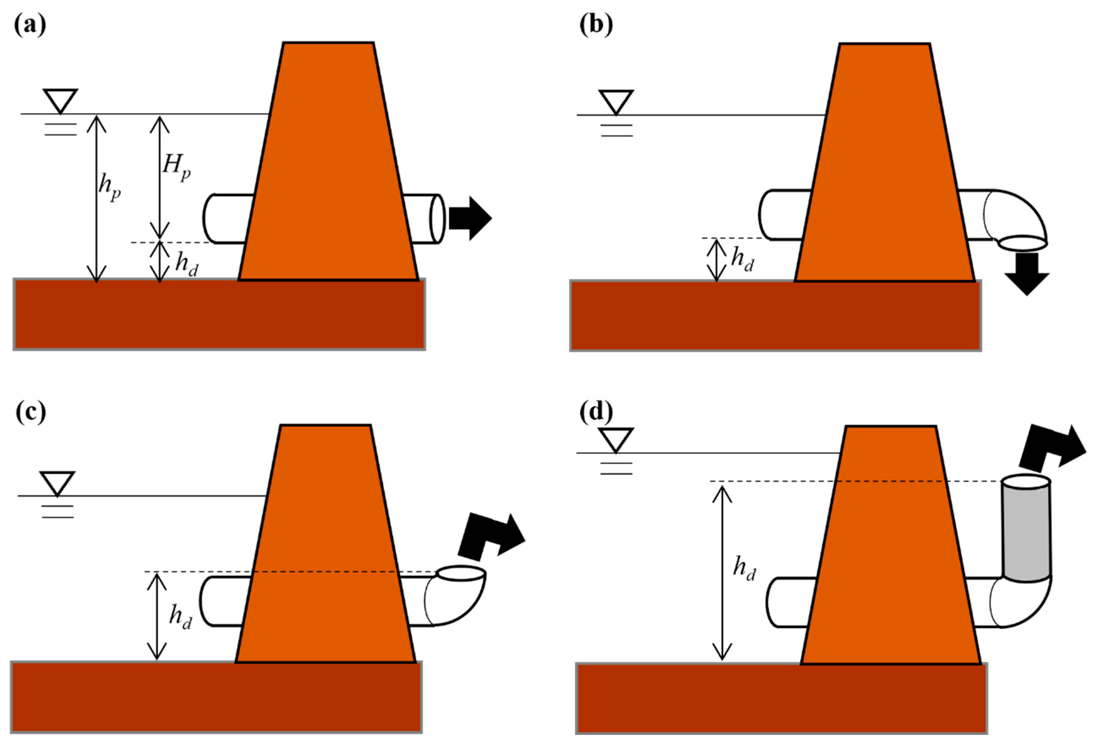
3.1.3. Evaluation of Drainage from Paddy Fields

The amount of drainage q_out from the paddy fields was set according to the paddy fields in the Kashima River basin, which is the target of this analysis. As shown in Figure 2, more than 80% of the paddy fields surveyed in the Kashima River basin were drained using circular free-draining pipes. A laboratory experiment was conducted to develop the relation between water level H_p and discharge Q_p (H-Q equation) for a circular free-draining pipe. For this, we selected a standard product pipe (VU75 manufactured by Kubota ChamiX Co., Ltd., Hyogo, Japan) with an inner diameter of 0.083 m, an outer diameter of 0.089 m, and a length of 2.00 m, which was similar to the circular pipe observed in the field. H_p is based on the lower end of the circular pipe, representing the reference plane. A large open channel (20 m long, 1.0 m wide, and 1.8 m high) owned by the Tokyo University of Science was equipped with a weir, and a vinyl chloride pipe was fitted onto the weir. The water level was kept constant on the inlet side, and the flow rate was measured on the outlet side using a bucket and stopwatch.

The results of the H-Q equation for various water levels (maximum 0.30 m) on the inlet side are shown in Figure 4. The H-Q equation was calculated separately for the open channel flow state and the pipe flow state. In the open channel flow state, the circular pipe has a water surface without becoming a full pipe flow (H_p ≤ 0.083 m). In the pipe flow state, the pipe is full (H_p > 0.083 m). Q_p is shown in Equation (7a,b).

Q_p = 0.1881 H_p² + 0.00858 H_p − 0.000018 (H_p ≤ 0.083 m)

(7a)

Q_p = −0.0982 H_p² + 0.06479 H_p − 0.002743 (0.083 m < H_p ≤ 0.30 m)

(7b)

Figure 4 shows that the equations adequately approximate the experimental data; however, some variation is observed in the H-Q relationship of the experimental data. In the present analysis, the bank height in the paddy field was set to a general value (=0.30 m) so that the applicable range of Equation (7b) was H_p ≤ 0.30 m. Given that the total rainfall in Section 3.3 in the analysis was less than 300 mm, the use of this equation was suitable for the scope of this study. Although it is preferable to determine the roughness of a pipe without using the H–Q relationship [Equation (7a,b)], the length of the pipe used in the present study was too short to create a uniform flow for both the open channel and pipe flows, and thus, we developed the H-Q relationship using the experimental data.

Equation (7a,b) were used to obtain the drainage q_out from the water level H_p in the paddy field. The spatial area of the paddy fields was not uniform, and the paddy field was divided into grids for this analysis. Therefore, setting the amount of drainage according to the spatial area of the paddy field in the grid was necessary. Given that the average area of one paddy field in the study area is $\overline{A_p}$= 1320 m², q_out is expressed as follows:

$$q_{out}=\frac{A_p}{\overline{A_p}}{Q}_p$$

(8)

where A_p is the area of the paddy field in the grid, and A_p is equal to the grid area when α₁ = 1. Using the area ratio $A_p/{\overline{A}}_p$, Equation (8) may satisfy the total discharge from the paddy fields in this area. In the actual paddy fields, even when circular pipes are used, the pipe diameters vary (Figure 2), thus causing the uncertainty in Equation (8). Certain drainage methods do not use circular pipes, and Equation (8) retains some uncertainties. These uncertainties in the evaluation of drainage should be addressed in future research.

3.1.4. Paddy Field Dam Model with Vertical Pipes

In this study, we examined a method for setting up a paddy field dam in accordance with the actual conditions of the paddy fields in the Kashima River basin. Drainage boxes are mostly used for drainage in paddy field dams. However, more than 80% of the paddy fields in the Kashima River basin are drained using circular pipes (Figure 2). In the case of drainage with circular pipes, numerous cases were observed in which straight pipes (Figure 5a) and a combination of straight and curved pipes were used (Figure 5b,c). In these cases, a simple method for increasing the paddy storage effect using circular pipes was effective, and it was consistent with the methods reported by Chai et al. [25]. As shown in Figure 5d, we focused on the outlet of the circular pipe. We considered a paddy field dam model where the outlet of the curved pipe faced upward and the outlet height h_d increased by adding vertical pipes to increase the paddy storage effect. This method was relatively simple and inexpensive and could be effective in cases where pipes are used for drainage. In this study, the effects of the paddy field dam were examined by changing the h_d values. In a study on paddy field dams using pipes [25], the cross-sectional area of the inlet side of the drainage pipes was narrow, and the height was increased, while the present method exhibited a simpler configuration.

3.2. Computational Procedures for a Preliminary Study of Paddy Field Division for Each Grid in This Model

The subgrid model is a new treatment for the water balance of a paddy field that reflects land use in the grid. Equation (3) was used for the water balance equation to derive Equation (5) in this model. The paddy fields were divided and integrated according to the calculation grid in this model. Therefore, a preliminary study was conducted to verify the validity of dividing and integrating paddy fields in each grid. In this study, water balance analyses were performed for the 10 paddy fields (Case P1), as shown in Figure 6. To validate the paddy field division, a water balance analysis was performed in which these 10 paddies were virtually regarded as a single paddy field (Case P2). These paddy fields were located in the Kashima River basin, which is the target for the analysis conducted in Section 3.3. In addition to the rainfall, vertical infiltration, and drainage in Equation (3), water exchange was observed between the adjacent paddies in the actual water balance of a paddy field.

$$\frac{d{h}_p}{dt}=r-f-q_{out}+{q^{\prime }}_{in}-{q^{\prime }}_{out}$$

(9)

where ${q^{\prime }}_{in}$ and ${q^{\prime }}_{out}$ are the inflows and outflows from the adjacent paddy fields, respectively. The drainage q_out to the drainage channel does not flow into the adjacent paddy fields (Figure 6). Assuming free drainage from the circular pipe, drainage q_out is expressed as follows:

$$q_{out}=\frac{Ca\sqrt{2g(h_p-h_d)}}{A_p}$$

(10)

where C is the coefficient of contraction, and a is the cross-sectional area of the drainage pipe. The inflow and outflow between the adjacent paddy fields are expressed in the same form as Equation (10). In this preliminary study, although Equation (7) could have been used for actual discharge to the drainage pipes in the basin, the simpler general Trichley equation was used.

The following equation was used as the water balance equation when 10 paddy fields were hypothetically considered to be a single paddy field by removing the water exchange with the adjacent paddies from Equation (9).

$$\frac{d{h}_p}{dt}=r-f-10\times q_{out}$$

(11)

Equation (8) was also used for the drainage volume; however, given that 10 paddy fields were regarded as a single paddy field, q_out was multiplied by 10, assuming there were 10 drainage pipes.

The elevation of the paddy fields decreased from No. 1 to 10 in Figure 6, and the water exchange between the paddy fields was based on elevation. The area A_p for each paddy field ranged from 738 to 1955 m², as shown in Figure 6. The other analysis conditions are presented in

Table 1. Computational conditions for water balance in the paddy fields in the preliminary study.

Variables	Unit	Value
C		0.65
a for qout	m2	7.85 × 10−3
a for q′in (q′out)	m2	1.963 × 10−4
hd	m	0.05
f	m/s	5.67 × 10−7

. The drainage pipe height h_d was 0.05 m, the diameter of the circular pipe for the drainage q_out was 0.05 m, and the pipe diameters for the inflow and outflow between the adjacent paddy fields (q′_in and q′_out) were assumed to be constant at 0.025 m, thus reflecting the conditions at the site. The infiltration intensity f was assumed to be constant (=5.67 × 10⁻⁷ m/s) without using the Green–Ampt model. The coefficient of contraction C was set to 0.65, which is in the general range. The rainfall conditions were set to constant over time for four patterns, namely, 5, 10, 15, and 20 mm/h, and calculations were performed for a period of 60 h. Initially, the paddy field was not flooded as the water depth was 0.

3.3. Main Calculation Procedures for Assessing the Effects of Paddy Field Dams on Flood Control in the Kashima River Basin Using the Present Model

To investigate the effect of the current paddy field storage and the introduction of paddy field dams on the reduction in the peak flood discharge in the Kashima River basin, rainfall–runoff analysis was conducted using the present model in the Kashima River basin in the main calculations. The grid width was 5 s (approximately 150 m), and the topographic data for elevation, flow direction, and the cumulative flow rate were upscaled to 5 s (approximately 150 m) from the 1 s resolution surface flow direction map of Japan [44]. The survey data provided by Chiba Prefecture were used to set the cross-sectional profile of the river channel grid from the mouth of Kashima River to 2.6 km at the confluence of the Takasaki River (Figure S2). In the upstream section, the cross-sectional profile was assumed to be rectangular because there were no cross-sectional survey data. The channel width W was given using catchment area A [30].

$$W=2A^{0.65}$$

(12)

The units for W and A are m and km², respectively. The depth of the rectangular cross-section was set to a high value where no inundation occurred because the inundation from the river channel to the surrounding area, which is provided by the RRI model, was not addressed. JAXA is the ALOS/AVNIR-2 high-resolution land use map (with a 10 m resolution for Japan, ver. 21.11, Figure 1) from the Earth Observation Research Center (EORC), and it was used as the land use condition [45]. In this high-resolution land-use map, land-use categories were classified into 12 types. However, in this analysis, the land-use categories were reclassified into the following four types: paddy fields, farmlands, forests, and urban areas. From these results, the land use area ratio α_i was calculated for each grid. The number of grids throughout the computational domain was 13,049, among which 7211 (55.3%) consisted of paddy fields.

Typhoon Bualoi, which occurred in 2019 and caused extensive flood damage in the Kashima River basin, was selected for computation. The computation period ranged from 0:00 on 25 October to 0:00 on 27 October (JST) in 2019. Radar/rain-gauge-analyzed precipitation (RRAP) data with 1 km of mesh and 30 min intervals were inputted as rainfall data. Three calculation cases were Case 0 without paddy storage, Case 1 with current paddy storage, and Case 2 with paddy field dams, as shown in

Table 2. Computational conditions for the assessment of the effects of paddy field dams on flood control in the Kashima River basin. Three cases are presented in the main calculations. The present subgrid model is not introduced in Case 0, where the water storage in the paddy fields was not considered. In Case 1, the current situation with h_d = 0.022 m was set using the present subgrid model. In Case 2, the effect of the paddy field dam with various h_d was examined using the present subgrid model.

Case	Condition	Height of Free-Drain Pipe hd [m]
0	No paddy field model
1	Current situation	0.022
2	Paddy field dam	0.05, 0.10, 0.15, 0.20, 0.25

. In Case 0, the water balance for the paddy field (Equation (3)) was not solved using the subgrid model because paddy storage was not considered, and the third term was excluded from Equation (5) as a continuous equation. The difference in the infiltration intensity according to land use was also considered in Case 0. In Case 1, the height of the free draining pipe h_d was set to 0.022 m, which was the average value in the current situation. In Case 2, where the paddy field dam was introduced, only h_d changed (0.05, 0.10, 0.15, 0.20, and 0.25 m). Here, the same h_d was assigned for all paddy field grids.

The model parameters for each land use category in the RRI model are shown in

Table 3. Numerical parameters of the rainfall–runoff–inundation (RRI) model for each land use type, namely paddy fields, croplands, residential areas, and forests. The roughness coefficient n, soil depth S_d, vertical and lateral infiltration coefficients k_v and k_a, respectively; porosity of saturated and unsaturated layers γ_a and γ_m, respectively; and suction S_f were set for each land use type.

Variables	Unit	Paddy Field	Farmland	Forest	Urban Area
Roughness coefficient n	m−1/3s	1.00	0.40	0.40	0.20
Soil depth Sd	m	1.00	1.00	2.00	1.00
Vertical infiltration coefficient kv	m/s	1.51 × 10−7	2.40 × 10−7		0
Lateral infiltration coefficient ka	m/s			0.15
Porosity of saturated layer γa		0.20	0.20	0.50	0.20
Porosity of unsaturated layer γm				0.05
Suction Sf	m	0.3163	0.239	0	0

, where n is the roughness coefficient, S_d is the soil depth, k_v and k_a are the vertical and lateral infiltration coefficients, respectively; γ_a and γ_m are the porosities of the saturated and unsaturated layer, respectively; and S_f represents suction. In the RRI model, the surface and seepage flows were calculated for each grid. Lateral infiltration was calculated for the forests, vertical infiltration was calculated for the paddy fields and farmlands, and no infiltration was calculated for urban areas. In paddy fields and farmlands, the vertical infiltration intensity was calculated using the Green–Ampt equation and k_v, γ_a, and S_f were included. In forests, the flow of seepage in saturated and unsaturated layers was calculated together, and k_a, γ_a, and γ_m were included. The roughness coefficient of the river channel was uniformly given as 0.035 m^−1/3s for all cross-sections. The RRI model manual [46] was used as a reference to determine the numerical parameters for the RRI model, as shown in Table 3. Certain numerical parameters need to be calibrated using sensitivity analysis for the 10 flood events, including Typhoon Bualoi in 2019, as shown in Table S1. The observed and calculated river discharge were compared at the Takaoka Bridge (2.8 km from the confluence of Kashima River, Figure 1b), where the observed discharge was available. The vertical infiltration coefficient k_v in paddy fields and farmlands was initially changed in the calculations. However, applying k_v used in previous studies (k_v = 5.56 × 10⁻⁷ m/s [47] and k_v = 8.33 × 10⁻⁷ m/s [48]), the runoff in the early stages of the flood was suppressed, resulting in poor reproducibility for the overall flood discharge. Therefore, a sensitivity analysis, where the vertical infiltration coefficient k_v was set relatively low and the porosity γ_a = 0.30−0.60 varied, was performed. The porosity γ_a was strongly related to the runoff volume for the forest area. The observed and calculated peak flows, as the most significant indexes, were compared, and the RMS value for the error in the calculated peak flows for the 10 flood events, Err_Qpeak, was found to be minimal at γ_a = 0.40−0.50 (Figure S3). At γ_a = 0.50, the calculated peak flow rate was generally consistent with the values observed in 2019 during Typhoon Bualoi (Figure 7). Therefore, we set γ_a = 0.50 for this calculation (Table 3).

4. Results

4.1. Preliminary Calculation for Determining the Effects of Paddy Field Division for Each Grid

To investigate the effects of dividing and integrating paddy fields on the water balance analysis results, the temporal changes in water depth for Cases P1 and P2 are shown in Figure 8. In Case P1, the arithmetic mean of the water depth in the 10 paddy fields is shown. The results of the two cases for the four rainfall patterns (r = 5, 10, 15, and 20 mm/h) are shown. In Case P1, the water depth increases linearly with time up to the drainpipe height h_d (=0.05 m) and then approaches a certain depth before reaching a steady state. The steady-state depth h_∞ increases as rainfall r increases. The water depth in Case P2 shows a similar pattern of temporal variation in Case P1. The increase in the initial depth and steady-state depth h_∞ in Case P2 is almost comparable with that in Case P1. In the phase where the water depth increases slowly and approaches the steady state (h_d < h < h_∞), the two cases are consistent with relatively low rainfall (r = 5 and 10 mm/h). However, for relatively high rainfall, r = 15 and 20 mm/h, the water depth in Case P2 slightly exceeded that in Case P1. The difference between the two cases is, at most, 3 mm, which is sufficiently small.

These calculations show that dividing and integrating paddy fields has little effect on the water balance analysis results. The water balance analysis is not affected by the division and integration of the paddy fields. This suggests that the drainage evaluation performed in Case P2 using Equation (11), which regards 10 paddy fields as a single paddy field, is generally valid. This multiple of 10 can also be expressed as the ratio of the total paddy field area to the average paddy field area for analysis. This verifies the basic validity of the drainage evaluation formula shown in Equation (8).

4.2. Results Obtained for the Main Calculations

4.2.1. River Discharge

To confirm the reproducibility of the river discharge in Case 1 of the current situation, the temporal variation in the observed and calculated river discharge at Takaoka Bridge on the Takasaki River and temporal and cumulative average rainfall values for the entire Kashima River basin (cumulative since 0:00, 25 October 2019) using RRAP are shown in Figure 9a,b. The observed discharge was obtained by converting the data from the observed water level and the site-specific rating curves between the water level and discharge. In this event, the rainfall started at approximately 6:00 on 25 October, peaked at 14:00 at an hourly rainfall of 56 mm, and almost stopped at 18:00. The total rainfall was 260 mm, which was the highest ever recorded for the Kashima River basin. The observed discharge at the Takaoka Bridge on the Takasaki River gradually increased on October 25 from 8:00 and reached its peak at approximately 19:00 (=192 m³/s), followed by a gradual decrease. However, the calculated discharge peaked at approximately 16:00 on October 25, which was earlier than the observed discharge, but the calculated peak flow rate (=189 m³/s) was almost the same between the calculated and observed values. Although it is desirable for the entire hydrograph to be consistent with the calculated and observed values, the present model reproduced acceptable values for the peak river discharges recorded for several flood events (Figure 7) but performed slightly less well in reproducing river discharge during floods. The same tendency was observed in the present calculation. Flood inundation occurred along the Kashima River and its tributary, the Takasaki River, following this heavy rainfall event. The fact that the present calculation did not take into consideration the inundation by deepening the riverbed may be one of the reasons why the hydrograph for the calculated discharge was sharper than that for the observed discharge. A further contributory factor in this regard may be the selection of numerical parameters in the RRI model, the assessment of which is an important focus in future studies. Despite the difficulty encountered in the present analysis with respect to reproducing the entire hydrograph, the reproduction of the peak flow rate was sufficiently effective to enable comparison among cases, and, accordingly, we focused on the peak flow rate when comparing the calculation results obtained for different cases.

To compare the discharge among the calculation cases, Figure 9c shows the time variation in the calculated discharges in Case 0 without considering paddy storage, the current situation (Case 1), and the introduction of the paddy field dam (Case 2) at the downstream end of Kashima River (the point of inflow into Lake Inba-numa). The pipe heights h_d of 0.022 m (Case 1) and 0.10, 0.20, and 0.25 m (all in Case 2) are illustrated. A comparison of the results of Case 0 and Case 1 revealed that the discharge increased relatively early, and the peak discharge for Case 0 exceeded that for Case 1. In the falling stage of the flood, the relationship between the relatively large and relatively small discharges changed at approximately 17:00 on October 25. Afterward, the discharge for Case 1 exceeded that for Case 0. The only difference between the two cases was whether the paddy storage was considered. This difference was caused by the effect of rainwater storage on the paddy fields. The delay in runoff and decrease in the peak discharge may have been caused by the current paddy field storage. Therefore, discharge from paddy fields must be appropriately modeled while accounting for paddy storage. For Cases 1 and 2, the peak discharge decreases as the pipe height increases despite the small difference in the rising stage. This indicates that the increase in the pipe height resulted in an increase in the paddy storage effect and contributed to the reduction in the river discharge downstream.

To quantitatively evaluate these results, the peak discharge Q_peak in all cases and the reduction rate R_Q for the peak discharge in each case with respect to the current condition (Case 1) were determined and are shown in Figure 10.

Here, all the results for Cases 0, 1, and 2 are displayed for the downstream end of the Kashima River. The peak discharge reduction rate R_Q was calculated using the following equation based on the value for Case 1, $Q_{peak1}$,

$$R_Q=\frac{Q_{peak1}-Q_{peak}\left(j\right)}{Q_{peak1}}\ast 100$$

(13)

The peak discharge of the target case was expressed as $Q_{peak}\left(j\right)$, and a positive value of R_Q indicated that the peak discharge decreased compared to that of Case 1. The peak discharge for Case 0 without paddy storage was +82 m³/s, and the reduction ratio R_Q was −14.6%. By contrast, the peak discharge for Case 2 with the paddy field dam was significantly reduced compared with that of Case 1, and the reduction ranged from 11 to 60 m³/s, with the reduction rate R_Q ranging from 2.0 to 10.5%. This reduction rate R_Q increased almost linearly as h_d increased up to 0.15 m, although it almost reached a plateau after h_d reached 0.20 m. Given that drainage begins when the water depth in the paddy field exceeds the pipe height h_d and assuming that infiltration was not considered, rainwater was only stored in the paddy field up to h_d from the beginning of the rainfall. In the present calculation, infiltration was considered, which allowed for the storage of rainfall that even slightly exceeded h_d. Given that the total rainfall was 260 mm during this heavy rainfall event, the discharge reduction rate for h_d ≥ 0.20 m at this rainfall scale was assumed to show no difference. The results show that the introduction of the paddy field dam has a pronounced effect on reducing the river discharge in the river downstream.

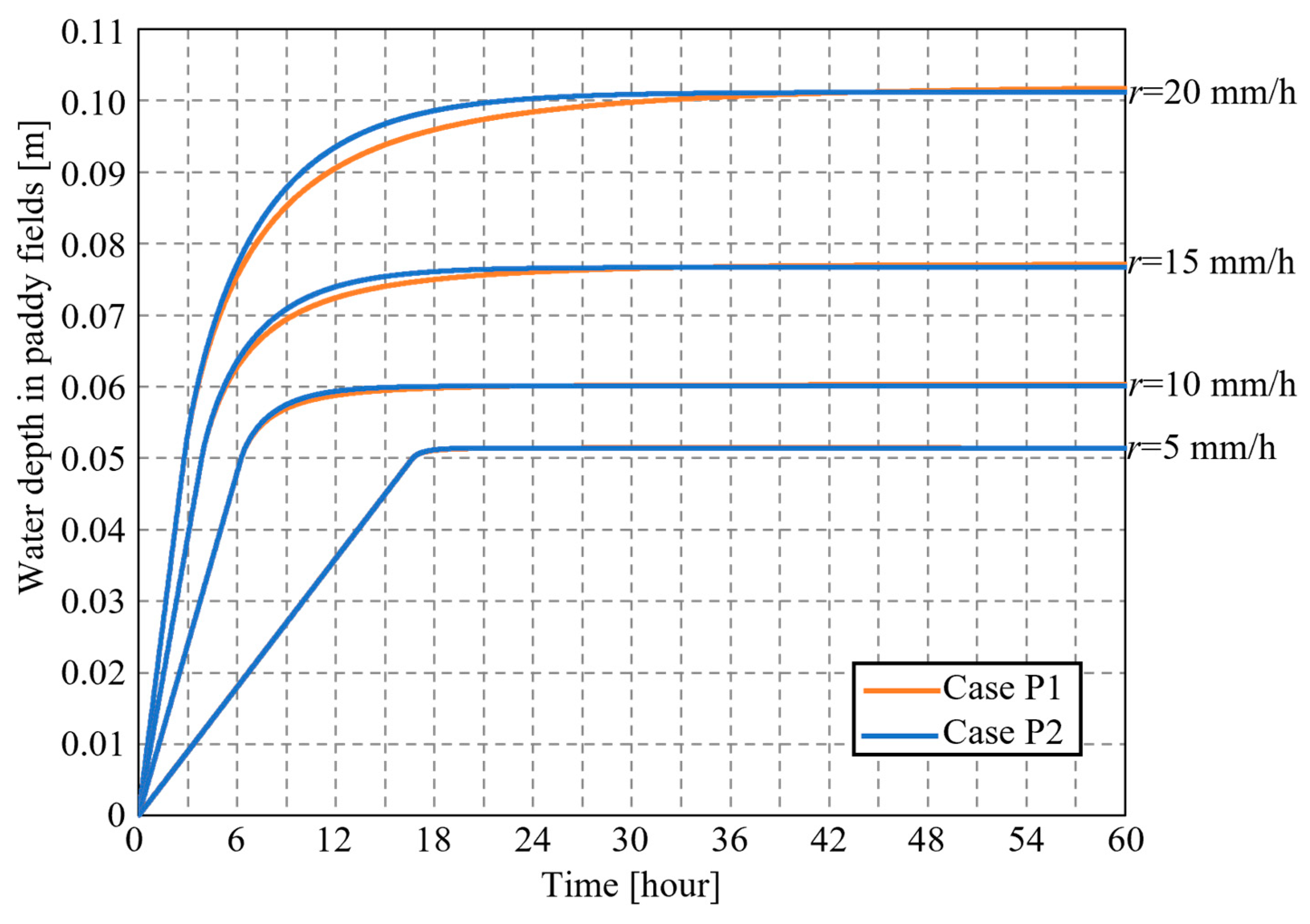
4.2.2. Water Depth in Paddy Fields

Figure 11a,b show the temporal variation in the calculated depth of paddy field h_p in the grids containing paddy fields and directly shows the effect of rainwater storage in the paddy fields. The value at Stn. A (Figure 1c, paddy field ratio α₁ = 91%) and the basin-averaged value are presented as an example. The results for Case 1 with a h_d of 0.022 m and Case 2 with various h_d values (0.05, 0.10, 0.15, 0.20, and 0.25 m) are shown in both figures. For Stn. A, the results from Case 0 without the paddy field model are also shown. The average hourly and cumulative rainfall in the basin (Figure 9a) are also shown. In the results for Stn. A, the water depth in Case 0 increased and decreased in line with the temporal change in the hourly rainfall, and the peak in the water depth (=0.115 m) was observed at 14:00 on October 25, which is the rainfall peak. However, in Case 1, the water depth at the beginning of the rainfall exceeded that in Case 0, and the peak water depth (=0.182 m) also exceeded that in Case 0. Therefore, the rainwater storage effect was clearly demonstrated. The results for various h_d values in Case 2 shows that the water depth in each condition was deeper with h_d, and the paddy storage effect was apparent with h_d. The peak water depths for each condition were 0.192, 0.209, 0.222, 0.230, and 0.231 m for h_d = 0.05, 0.10, 0.15, 0.20, and 0.25 m, respectively. These values were all lower than the bank height of 0.30 m. In the case of h_d = 0.25 m, the peak water depth was below h_d; therefore, no drainage occurred from the circular pipe, and vertical infiltration was the only runoff from the paddy field. In the case of h_d = 0.20 m, the water depth exceeded h_d, including the peak water depth; however, the water depth was consistent with that at h_d = 0.25 m. This was attributed to the smaller discharge from the circular pipe under the present rainfall conditions.

The basin-averaged paddy field depth (Figure 11b) is similar to that of Stn. A. However, the peak values vary owing to the difference in rainfall patterns (Figure S1). The results show that the subgrid model can adequately reproduce the storage effect in paddy fields. The water depths in the paddy fields vary significantly from those using general runoff models, which do not reflect the storage effect in paddy fields. The introduction of the paddy field dam led to increased water depth in the paddy field and subsequently increased the paddy storage capacity.

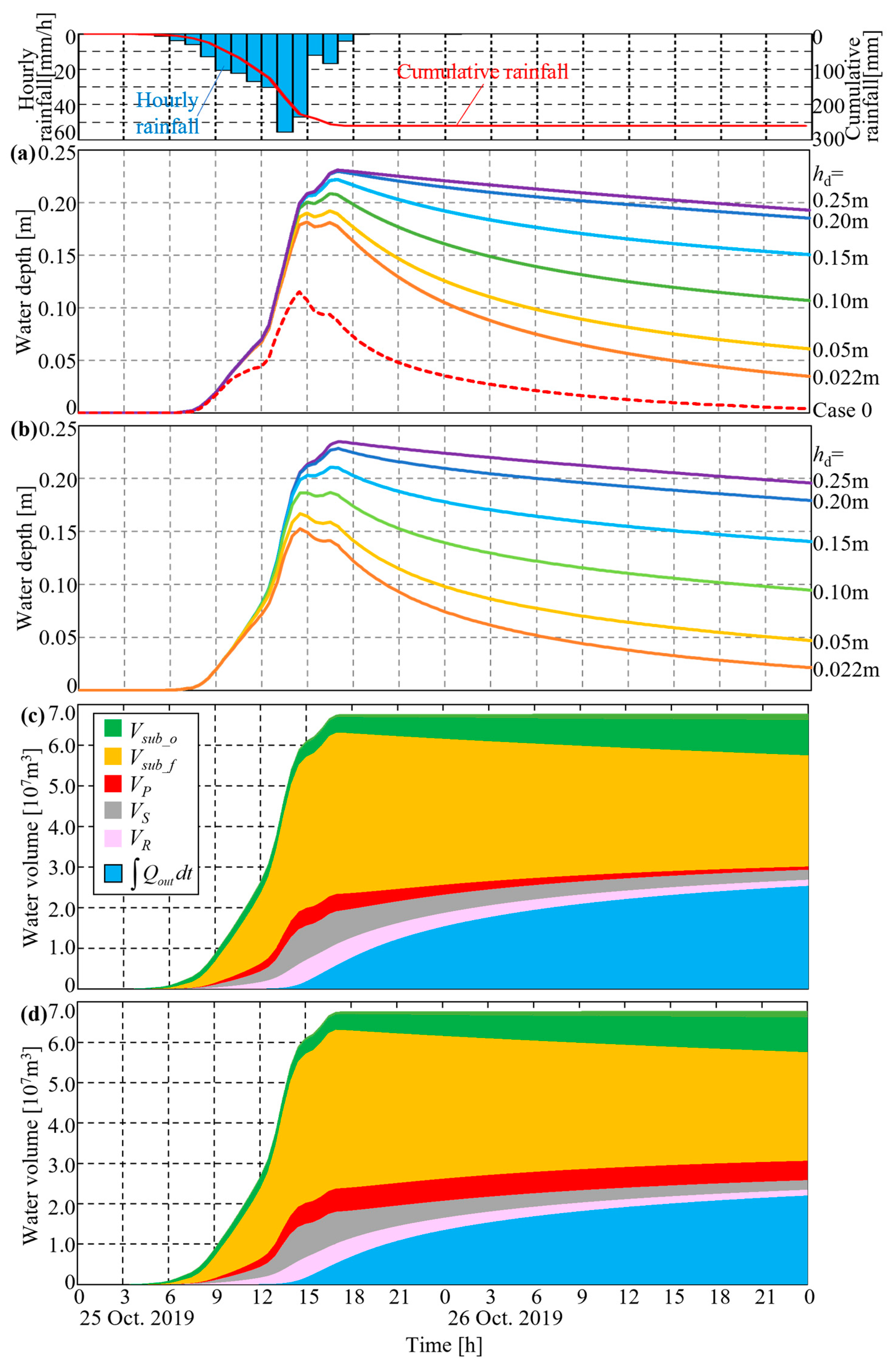
4.2.3. Water Balances at the Basin Scale

To understand the effect of paddy field storage on the water balance characteristics of the entire basin, the temporal changes in the water volume throughout the basin are shown in Figure 11c,d. Here, the water volume is divided into river storage V_R, surface flow storage V_S, paddy field storage V_P, the sub-surface volume in forests V_sub-f, and the cumulative volume of vertical infiltration in paddy fields and farmlands V_sub-o. The remaining volume is the cumulative discharge at the downstream end of the basin ${\displaystyle \int Q_{out}dt}$. The summation of these volumes is equal to the cumulative rainfall ${\displaystyle \int RAdt}$:

$${\displaystyle \int RAdt}={\displaystyle \int Q_{out}dt}+V_R+V_S+V_P+V_{Sub-f}+V_{sub-o}$$

(14)

where R is the basin-mean rainfall, A is the basin area, and Q_out is the downstream discharge. The results from Case 1 (h_d = 0.022 m) and Case 2 (h_d = 0.25 m) are illustrated in Figure 11c,d, respectively. The results from Case 1 indicate that the sub-surface volume in the forest V_sub-f is dominant, and V_sub-o also increases over time. The paddy field storage V_P is significant from the early stage of the rainfall with the surface flow storage V_S. The paddy storage V_P and the surface flow storage V_S increased rapidly from 13:00 to 15:00 on October 25, when the hourly rainfall increased. The river storage V_R and cumulative discharge at the downstream end ${\displaystyle \int Q_{out}dt}$ also increased with a time delay from V_P and V_S. By contrast, in Case 2, when h_d was 0.25 m, the paddy field storage increased compared to Case 1. This increase continued throughout the rainfall peak and the falling stage. Instead of an increase in paddy field storage, a decrease was observed in the river storage and downstream end discharge. Therefore, in the context of water balance, the effect of paddy storage was significant in the current situation for the paddy fields. The effects of paddy storage become more pronounced upon the introduction of the paddy field dam.

A comparison of the temporal changes in the water volume for each type is shown in Figure 12. Here, the results for h_d = 0.022, 0.10, and 0.25 m are shown for ${\displaystyle \int Q_{out}dt}$, V_R, V_S, and V_P. The results for V_sub-f and V_sub-o are omitted here because they exhibit almost no difference. The scale of the vertical axis was not standardized and was adjusted to a size where it was easy to identify the difference between cases. Notably, ${\displaystyle \int Q_{out}dt}$ decreased as h_d increased (Figure 12a), which corresponds to previous results (Figure 9). The difference between the cases for ${\displaystyle \int Q_{out}dt}$ increased over time. In contrast, V_R decreased as h_d increased, which was consistent with the trend for ${\displaystyle \int Q_{out}dt}$ (Figure 12b). V_S shows almost no difference among the cases (Figure 12c). V_P increased with increasing h_d (Figure 12d), and consequently, the sum of ${\displaystyle \int Q_{out}dt}$, V_R, and V_P was almost consistent among the cases (Figure 12e). Based on the water balance characteristics, the improvement in the paddy field storage effect decreased the river channel storage and, therefore, the river discharge. The peak values for paddy storage were 4.39 × 10⁶ m³, 5.10 × 10⁶ m³, and 5.76 × 10⁶ m³ at h_d values of 0.022, 0.10, and 0.25 m, respectively. This suggests that a significant rainwater storage effect was demonstrated in Case 1 under the present conditions.

5. Discussion

The subgrid model developed in this study can quantitatively evaluate the effect of the current paddy storage and introduction of the paddy field dams as a flood control measure throughout the basin. The results using the subgrid model highlight that the rainwater storage effect for the current paddy field leads to a reduction in the peak river discharge. The paddy field storage effect becomes more pronounced when the height of the drainage pipe in the paddy field dam is increased, thus contributing to a reduction in the river discharge. This finding has been confirmed by the water balance characteristics for the entire basin and the depth of the paddy fields.

One of the most important findings from the main calculation is that the peak river discharge was reduced by 14.6% in the present paddy field compared with Case 0 without paddy storage (Figure 9 and Figure 10). This highlights the importance of controlling the increase in abandoned land and the conversion of paddy fields to other land uses. In the general runoff model, the unit width flow q_x, q_y in the paddy field is a function of the water-level gradient based on diffusion wave approximation as well as other land uses. The rainwater that falls on the paddy field runs off rapidly along the topographic and water-level gradients. However, in the actual paddy fields surrounded by banks, rainwater is stored and then drained from the drainage pipes or boxes. This could delay the runoff and reduce river discharge in the downstream area. The present subgrid model can adequately describe paddy storage based on the drainage process of the paddy field, which should be included in models that are configured for runoff analysis and include paddy field areas.

In addition, the reduction rate of the peak river discharge R_Q at h_d = 0.25 m was 10.5% greater than the ratio of the paddy field area to the total basin area (=7.5%). When h_d = 0.25 m, the drainage pipe height h_d exceeded the paddy field depth throughout the flood period so that the drainage q_out from the paddy field was zero. This is equivalent to a decrease in the paddy surface area, which is assumed to correspond with the rate of decrease in the peak discharge. However, the rate of decrease in the peak discharge (10.5%) exceeded that of the paddy area (7.5%). To verify this factor in detail, a correlation diagram between the reduction rate of the peak discharge R_Q and the paddy field area ratio α₁ in each catchment area is shown in Figure 13. The data in this figure were collected from the upstream to the downstream points of the Kashima River and its tributary, the Takasaki River. The peak discharge reduction rate R_Q exceeded the paddy field area ratio α₁ at all points. This trend is more pronounced in the mainstem of the Kashima River than in the Takasaki River. An approximate straight line was applied to R_Q and α₁ data for the Kashima River and Takasaki River (dotted line in the figure). The slope was 1.493 with an R² = 0.996 for the Kashima River and 1.222 with an R² = 0.998 for the Takasaki River. The results from the t-test on the data showed that p < 0.01 for both rivers and the linear relationship between R_Q and α₁ was confirmed to be significant for both rivers. Therefore, the peak flow reduction rate exceeded the paddy field area ratio, and this difference increased with the paddy field area ratio throughout the Kashima River basin. The fundamental mechanism for this phenomenon is that the river volume V_R decreases owing to the enhancement of rainwater storage in the paddy fields (Figure 12), and the water-level gradient in the river also decreases. Therefore, the discharge based on the diffusion wave approximation also decreases. Originally, the water volume V_S of the surface flow was assumed to decrease owing to paddy field storage. However, in the Kashima River basin, paddy fields are located along the river (Figure 1c). Therefore, paddy field storage directly affects the river flow and has relatively little effect on the surface flow water volume (Figure 12).

The slope of the approximate equation for both rivers was larger for the Kashima River (=1.493) than for the Takasaki River (=1.222) because the rainfall over the main channel of the Kashima River exceeded that of the Takasaki River, as shown in Figure S1. However, when the rainfall increased and the water level in the paddy fields exceeded the height of the bank, the rainwater storage in the paddy fields no longer made an impact. The paddy storage effect was affected by the rainfall pattern, and there was optimal maximum rainfall for the paddy field dams [22].

The calculated results present certain uncertainties. The drainage process in the model is based on the data measured from certain drainage pipes in the local paddy field, and the mean values for the pipe diameters and heights are presented uniformly. Collecting detailed data from paddy fields and inputting them into the computational model is necessary and considerably labor intensive, which should be investigated in further studies. General parameters are given for vertical infiltration in paddy fields. However, this model does not assume that vertical infiltration is enhanced in areas where culvert drainage has been constructed, and the drainage discharges to downstream rivers. This model assumes that culvert drainage has not been considered. It is important to close the culvert drainage constructed in paddy fields to maintain the paddy storage effects. Model calibration was performed based on a comparison of the calculated and observed discharges at a single station along the Takasaki River. In future studies, it is necessary to verify the validity of the calculated results for a comparison of the observed data in water elevation and discharge within the entire Kashima River basin.

6. Conclusions

In this study, we developed a subgrid model for the quantitative evaluation of flood control measures based on RBDRSA throughout a basin, which can evaluate the paddy water balance while considering land use distribution on a computational grid. The subgrid model was incorporated into the RRI model. Based on this model, the effects of current paddy storage and the introduction of paddy field dams on the reduction in river flood discharge were examined in the Kashima River basin. The main study findings are as follows.

(1)

The fundamental concepts of the subgrid model to overcome the issues of the existing runoff models are to (a) maintain the general grid-based distributed rainfall–runoff model framework, (b) reflect the detailed land use in the computational grid, and (c) appropriately account for the effect of the paddy field storage. Fundamental equations are separately derived for paddy and non-paddy fields; however, the basic form of the RRI model remains unchanged. The subgrid model can be used to evaluate the storage effect of paddy field dams without losing the computational framework of the runoff model.

(2)

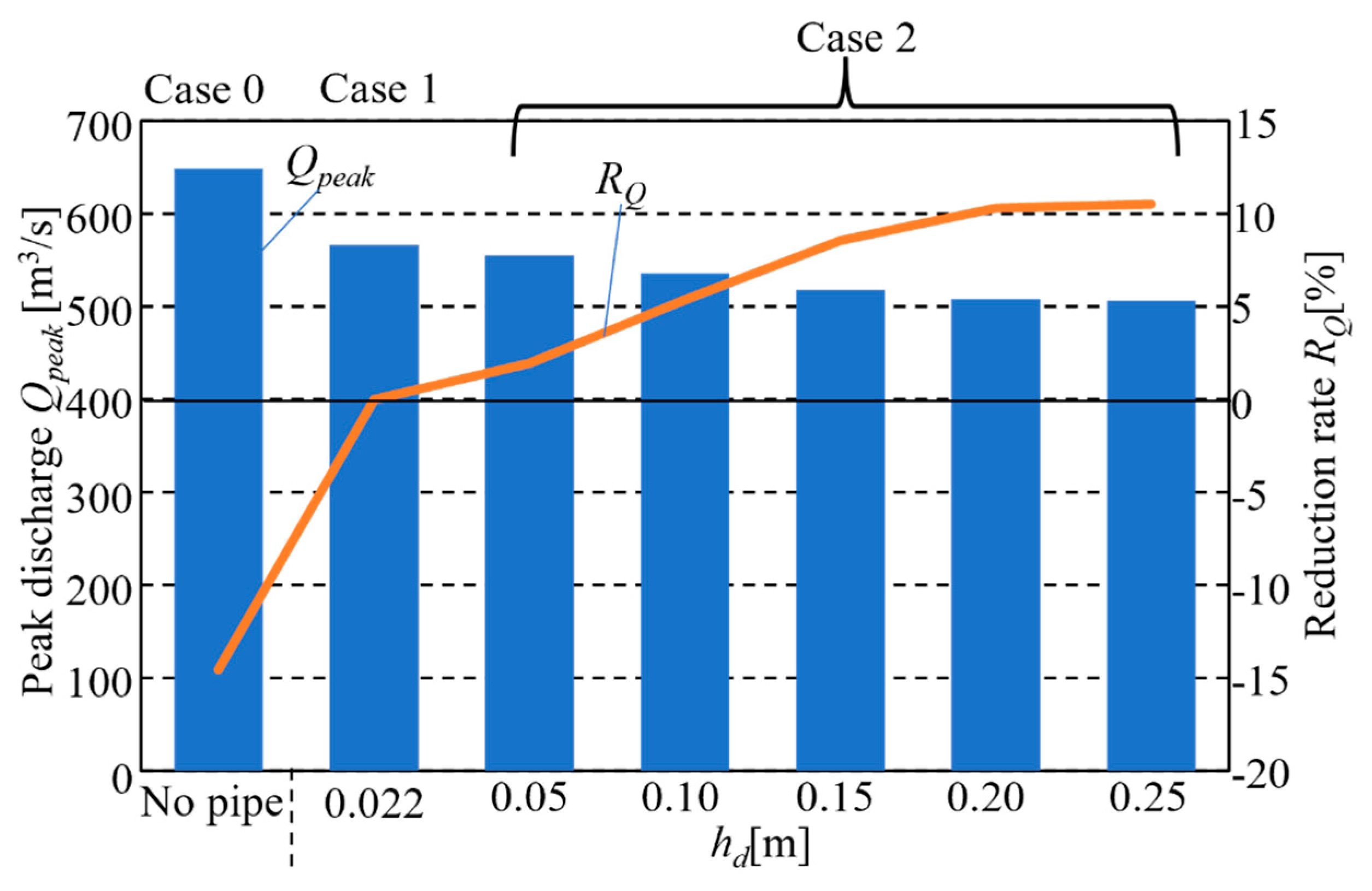
To investigate the effect of current paddy field storage and the introduction of a paddy field dam on the reduction in peak flood discharge, rainfall–runoff analysis was conducted in the Kashima River basin using the model developed in this study. The model parameters were calibrated to fit the peak river discharge through the runoff simulations for ten flood events in the Kashima River basin. The computational results highlighted that the rainwater storage effect of the current paddy field reduces the peak river discharge significantly, thereby suggesting that the drainage process of the paddy field should be incorporated into a model configuration for runoff analysis, including the paddy field area. Notably, the paddy field storage effect became more pronounced when the height of the drainage pipe in the paddy field dam increased.

(3)

To understand the effect of paddy field storage on the water balance characteristics of the entire basin, temporal changes in water volume throughout the basin were examined. Based on the water balance characteristics, the improvement in the paddy field storage effect decreases the river channel storage and, consequently, the river discharge.

The calculated results using the present subgrid model quantitatively show the flood control effect of paddy field storage over the entire basin. Therefore, the proposed subgrid model can be a useful tool for promoting new basin-level control measures.

References

1. Rahmayanti, K.P.; Azzahra, S.; Arnanda, N.A. Actor-Network and Non-Government failure in Jakarta flood disaster in January 2020. IOP Conf. Ser. Earth Environ. Sci. 2021, 716, 012053. [Google Scholar] [CrossRef]
2. Zhou, Z.Q.; Xie, S.P.; Zhang, R. Historic Yangtze flooding of 2020 tied to extreme Indian Ocean conditions. Proc. Natl. Acad. Sci. USA 2021, 118, e2022255118. [Google Scholar] [CrossRef] [PubMed]
3. Koks, E.; Van Ginkel, K.; Van Marle, M.; Lemnitzer, A. Brief Communication: Critical Infrastructure impacts of the 2021 mid-July western European flood event. Nat. Hazards Earth Syst. Sci. 2021, 22, 3831–3838. [Google Scholar] [CrossRef]
4. Cabinet Office (Government of Japan). On Disaster Damage by the Heavy Rainfall in July 2018. 2018. Available online: http://www.bousai.go.jp/updates/h30typhoon7/pdf/310109_1700_h30typhoon7_01.pdf (accessed on 23 June 2022). (In Japanese).
5. Cabinet Office (Government of Japan). On Disaster Damage by the Typhoon No. 19 (Hagibis) in 2019; Cabinet Office (Government of Japan): Tokyo, Japan, 2019. (In Japanese) [Google Scholar]
6. Cabinet Office (Government of Japan). On Disaster Damage by the Heavy Rainfall in July 2020. 2020. Available online: http://www.bousai.go.jp/updates/r2_07ooame/pdf/r20703_ooame_40.pdf (accessed on 23 June 2022). (In Japanese).
7. Kawase, H.; Imada, Y.; Tsuguti, H.; Nakaegawa, T.; Seino, N.; Murata, A.; Takayabu, I. The heavy rain event of July 2018 in Japan enhanced by historical warming. Bull. Am. Meteorol. Soc. 2020, 101, S109–S114. [Google Scholar] [CrossRef]
8. Kawase, H.; Yamaguchi, M.; Imada, Y.; Hayashi, S.; Murata, A.; Nakaegawa, T.; Miyasaka, T.; Takayabu, I. Enhancement of extremely heavy precipitation induced by Typhoon Hagibis (2019) due to historical warming. Sci. Online Lett. Atmos. 2021, 17A, 7–13. [Google Scholar] [CrossRef]
9. IPCC AR6. Climate Change 2021: AR6 Synthesis Report. 2021. Available online: https://www.ipcc.ch/report/sixth-assessment-report-cycle/ (accessed on 23 June 2022).
10. Ministry of Land Infrastructure, Transport and Tourism (MLIT). River Basin Disaster Resilience and Sustainability by All. 2020. Available online: https://www.mlit.go.jp/river/kokusai/pdf/pdf21.pdf (accessed on 23 June 2022).
11. Abler, D. Multifunctionality, agricultural policy, and environmental policy. Agric. Econ. Res. Rev. 2004, 33, 8–17. [Google Scholar] [CrossRef]
12. Groenfeldt, D. Multifunctionality of agricultural water: Looking beyond food production and ecosystem services. Irrig. Drain. 2006, 55, 73–83. [Google Scholar] [CrossRef]
13. Wu, R.S.; Sue, W.R.; Chien, C.B.; Chen, C.H.; Chang, J.S.; Lin, K.M. A simulation model for investigating the effects of rice paddy fields on the runoff system. Math. Comput. Model. 2001, 33, 649–658. [Google Scholar] [CrossRef]
14. Huang, C.C.; Tsai, M.H.; Lin, W.T.; Ho, Y.F.; Tan, C.H. Multifunctionality of Paddy fields in Taiwan. Paddy Water Environ. 2006, 4, 199–204. [Google Scholar] [CrossRef]
15. Masumoto, T.; Yoshida, T.; Kubota, T. An index for evaluating the flood prevention function of paddies. Paddy Water Environ. 2006, 4, 205–210. [Google Scholar] [CrossRef]
16. Matsuno, Y. Prospects for multifunctionality of paddy rice cultivation in Japan and other countries in monsoon Asia. Paddy Water Environ. 2006, 4, 189–197. [Google Scholar] [CrossRef]
17. Kim, T.C.; Gim, U.S.; Kim, J.S.; Kim, D.S. The multi-functionality of paddy farming in Korea. Paddy Water Environ. 2006, 4, 169–179. [Google Scholar] [CrossRef]
18. Kim, J.O.; Lee, S.H.; Jang, K.S. Efforts to improve biodiversity in the paddy field ecosystem of South Korea. Reintroduction 2011, 1, 25–30. Available online: http://www.stork.u-hyogo.ac.jp/downloads/journal/01_05.pdf (accessed on 23 June 2022).
19. Sujono, J. Flood reduction function of paddy rice fields under different water saving irrigation techniques. J. Water Resour. 2010, 2, 555–559. [Google Scholar] [CrossRef]
20. Hao, L.; Sun, G.; Liu, Y.; Wan, J.; Qin, M.; Qian, H.; Liu, C.; Zheng, J.; John, R.; Fan, P.; et al. Urbanization dramatically altered the water balances of a paddy. Hydrol. Earth Syst. Sci. 2015, 19, 3319–3331. [Google Scholar] [CrossRef]
21. Yoshikawa, N.; Nagao, N.; Misawa, S. Evaluation of the flood mitigation effect of a Paddy Field Dam project. Agric. Water Manag. 2010, 97, 259–270. [Google Scholar] [CrossRef]
22. Miyazu, S.; Matsushita, T.; Iwamura, Y.; Yoshikawa, N. Study on limit of flood mitigation effect of paddy field dam. Eng. Ser. B1 Hydraul. Eng. 2020, 76, I_805–I_810. (In Japanese) [Google Scholar] [CrossRef]
23. Kobayashi, K.; Kono, Y.; Kimura, T.; Tanakamaru, H. Estimation of paddy field dam effect on flood mitigation focusing on Suse region of Hyogo, Japan. Hydrol. Res. Lett. 2021, 15, 64–70. [Google Scholar] [CrossRef]
24. Chen, R.; Cheng, Y.; Huang, P. A suitable design of outlet type for paddies in Taiwan by evaluating the flood detention effect and applicability. Irrig. Drain. Syst. 2019, 68, 937–949. [Google Scholar] [CrossRef]
25. Chai, Y.; Touge, Y.; Shi, K.; Kazama, S. Evaluating potential flood mitigation effect of paddy field dam for Typhoon No. 19 in 2019 in the Naruse River basin. Eng. Ser. B1 Hydraul. Eng. 2020, 76, 295–303. [Google Scholar] [CrossRef]
26. Abbott, M.B.; Bathurst, J.C.; Cunge, J.A.; O’Connell, P.E.; Rasmussen, J. An introduction to the European Hydrological System-Systeme Hydrologique European. ‘SHE’, 1: History and philosophy of a physically based distributed modelling system. J. Hydrol. 1986, 87, 45–59. [Google Scholar] [CrossRef]
27. Abbott, M.B.; Bathurst, J.C.; Cunge, J.A.; O’Connell, P.E.; Rasmussen, J. An introduction to the European Hydrological System-Systeme Hydrologique European, ‘SHE’, 2: Structure of a physically based distributed modelling system. J. Hydrol. 1986, 87, 61–77. [Google Scholar] [CrossRef]
28. Jia, Y.W.; Ni, G.H.; Yoshihisa, K. Development of WEP model and its application in urban area. Hydrol. Process 2001, 15, 2175–2194. [Google Scholar] [CrossRef]
29. Noh, S.J.; Tachikawa, Y.; Shiiba, M.; Kim, S. Ensemble Kalman filtering and particle filtering in a lag-time window for short-term streamflow forecasting with a distributed hydrologic model. J. Hydrol. 2013, 18, 1684–1696. [Google Scholar] [CrossRef]
30. Sayama, T.; Ozawa, G.; Kawakami, T.; Nabesaka, S.; Fukami, K. Rainfall-runoff-inundation analysis of the 2010 Pakistan flood in the Kabul River basin. Hydrol. Sci. J. 2012, 57, 298–312. [Google Scholar] [CrossRef]
31. Wang, S.; Zhang, Z.; Sun, G.; Strauss, P.; Guo, J.; Tang, Y.; Yao, A. Multi-site calibration, validation, and sensitivity analysis of the MIKE SHE Model for a large watershed in northern China. Hydrol. Earth Syst. Sci. 2012, 16, 4621–4632. [Google Scholar] [CrossRef]
32. Jia, Y.; Wang, H.; Zhou, Z.; Qiu, Y.; Luo, X.; Wang, J.; Yan, D.; Qin, D. Development of the WEP-L distributed hydrological model and dynamic assessment of water resources in the Yellow River basin. J. Hydrol. 2006, 331, 606–629. [Google Scholar] [CrossRef]
33. Leonarduzzi, E.; Maxwell, R.M.; Mirus, B.B.; Molnar, P. Numerical analysis of the effect of subgrid variability in a physically based hydrological model on runoff, soil moisture, and slope stability. Resour. Res. 2021, 57, e2020WR027326. [Google Scholar] [CrossRef]
34. Antoine, M.; Javaux, M.; Bielders, C.L. Integrating subgrid connectivity properties of the micro-topography in distributed runoff models, at the interrail scale. J. Hydrol. 2011, 403, 213–223. [Google Scholar] [CrossRef]
35. Beldring, S.; Engeland, K.; Roald, L.A.; Sælthun, N.R.; Voksø, A. Estimation of parameters in a distributed precipitation-runoff model for Norway. Hydrol. Earth Syst. Sci. 2003, 7, 304–316. [Google Scholar] [CrossRef]
36. Hagemann, S.; Gates, L.D. Improving a subgrid runoff parameterization scheme for climate models by the use of high-resolution data derived from satellite observations. Dynamics 2003, 21, 349–359. [Google Scholar] [CrossRef]
37. Liang, X.; Xie, Z. A new surface runoff parameterization with subgrid-scale soil heterogeneity for land surface models. Adv. Water Resour. 2001, 24, 1173–1193. [Google Scholar] [CrossRef]
38. Neal, J.; Schumann, G.J.-P.; Bates, P.D. A simple model for simulating river hydraulics and floodplain inundation over large and data sparse areas. Water Resour. Res. 2012, 48, W11506. [Google Scholar] [CrossRef]
39. Jung, I.K.; Park, J.Y.; Park, G.; Lee, M.S.; Kim, S.J. A grid-based rainfall-runoff model for flood simulation including paddy fields. Paddy Water Environ. 2011, 9, 275–290. [Google Scholar] [CrossRef]
40. Sayama, T.; Tatebe, Y.; Tanaka, S. An emergency response-type rainfall runoff-inundation simulation for 2011 Thailand floods. J. Flood Risk Manag. 2015, 10, 65–78. [Google Scholar] [CrossRef]
41. Yamashita, A. Mesh Data Analysis of Watershed Environment Focusing on Land Use and Water Supply-demand. Environ. Sci. 2019, 32, 36–45, (In Japanese with English abstract). [Google Scholar]
42. Chiba Prefecture. The 18th Chiba Prefecture Disaster Countermeasures Headquarters Meeting. 2019. Available online: https://www.pref.chiba.lg.jp/bousai/bousai/documents/kaigi18-2.pdf (accessed on 23 June 2022). (In Japanese).
43. Rawls, W.J.; Ahuja, L.R.; Brakensiek, D.L.; Shirmohammadi, A. Infiltration and soil water movement. In Handbook of Hydrology; McGraw-Hill: New York, NY, USA, 1992; pp. 5.1–5.52. [Google Scholar]
44. Yamazaki, D.; Togashi, S.; Takeshima, A.; Sayama, T. High-resolution flow direction map of Japan. J. Jpn. Soc. Civ. Eng. Ser. B1 Hydraul. Eng. 2020, 8, 234–240. [Google Scholar] [CrossRef]
45. Shimada, M.; Isoguchi, O.; Motooka, T.; Shiraishi, T.; Mukaida, A.; Okumura, H.; Otaki, T.; Itoh, T. Generation of 10 m resolution PALSAR and JERS-SAR mosaic and forest/non-forest maps for forest carbon tracking. In Proceedings of the 2011 IEEE International Geoscience and Remote Sensing Symposium, Vancouver, BC, Canada, 24–29 July 2011; pp. 3510–3513. [Google Scholar]
46. International Center for Water Hazard and Risk Management (ICHARM). Rainfall–Runoff Inundation Model User’s Manual ver. 1.4.2.4. 2021. Available online: https://www.pwri.go.jp/icharm/research/rri/rri_top.html (accessed on 23 June 2022).
47. Shimizu, R.; Kaida, K.; Matsuda, M.; Uchida, T.; Sayama, T.; Kawahara, Y. Enhanced rainfall-runoff-flood simulation with RRI model incorporating river vegetation resistance based on 2D numerical calculation results and slope direction surface flow flux. J. Jpn. Soc. Civ. Eng. Ser. B1 Hydraul. Eng. 2021, 77, 84–91, (In Japanese with English abstract). [Google Scholar] [CrossRef]
48. Yamamoto, K.; Sayama, T.; Konja, A.; Nakamura, Y.; Miyake, S.; Tanaka, K. Integrated analysis of rainfall-runoff and flood inundation by the RRI model in the Chikusa River basin. J. Jpn. Soc. Nat. Disaster Sci. 2017, 36, 139–151, (In Japanese with English abstract). [Google Scholar]
Figure 1. Locations of the study sites, Lake Inba-numa and Kashima River basins (a), and maps showing elevation (b) and land use (c) in the Kashima River basin. A red triangle shows the location of the river discharge observatory along the Takasaki River.
Water 16 00255 g001
Figure 2. Images of typical drainage systems used in paddy fields (a) and box plots of the pipe height, pipe diameter, and bank height at the Kashima River basin (b). Solid lines represent the mean values; the tops and bottoms of the boxes denote the 75% and 25% quartiles, respectively; the tops and bottoms of the error bars show the maximum and minimum values, excluding outliers. Crosses denote the mean data values. The field data were collected from 174 paddy fields in the Kashima River basin in 2021.
Water 16 00255 g002
Figure 3. Schematic of the fundamental concept of the subgrid model for water storage in paddy fields. This subgrid model maintains the general framework of a distributed rainfall–runoff model (a), accurately incorporates subgrid scale variation in land use in each grid (b), and calculates the water storage for the paddy field (c).
Water 16 00255 g003
Figure 4. Rating curves for the water level Hp and outflow discharge Qp obtained in the laboratory experiment using a polyvinyl chloride (PVC) pipe. The rating curves were divided based on water levels lower or higher than the pipe diameter (0.083 m). The dashed lines represent approximation curves for the data measured.
Water 16 00255 g004
Figure 5. Schematic of the general pipe arrangement for outflow from a paddy field (ac) and the paddy field dam model in this study (d). Illustrations of hp, hd, and Hp are shown in (a). In the present model, the vertical pipe presented in gray was also connected.
Water 16 00255 g005
Figure 6. Site of the preliminary study with ten paddy fields near the Kashima River. White arrows show the outflow from the paddy fields into the drainage channel. Blue arrows show the inflow and outflow between adjacent paddy fields. The spatial area of each of the ten paddy fields is shown in the table.
Water 16 00255 g006
Figure 7. Comparison of the observed and calculated peak discharge at Takaoka Bridge on the Takasaki River. Porosity γa was set to 0.50. The data shown are obtained from the 10 flood events listed in Table S1.
Water 16 00255 g007
Figure 8. Time series analysis of the water depth in paddy fields for Cases P1 and P2 in the preliminary calculation.
Water 16 00255 g008
Figure 9. Temporal variation in the hourly and cumulative rainfall averages in the Kashima River basin (a), the observed and calculated river discharge at Takaoka Bridge on the Takasaki River (b), and the calculated river discharge at the downstream point of the Kashima River (c). The rainfall data are based on the radar/rain gauge-analyzed precipitation (RRAP).
Water 16 00255 g009
Figure 10. Peak discharge Qpeak at the downstream point of Kashima River for all cases is shown in the bar graph, and its reduction rate RQ from Case 1 results is shown in the line graph. The horizontal axis shows the height of the free draining pipe hd, where 0.022 m and 0.05–0.25 m correspond to the results of Case 1 and Case 2, respectively. “No pipe” in the horizontal axis refers to the results of Case 0.
Water 16 00255 g010
Figure 11. Temporal variation in water depth calculated for the paddy fields at Stn. A, as shown in Figure 1a, and the basin-averaged water depth (b). The results calculated for Case 0 and Case 1, for which hd = 0.022 m, and Case 2, for which hd = 0.05, 0.10, 0.15, 0.20, and 0.25 m, are shown in (a) and (b), respectively. Temporal variations in the water volume across the entire basin for the results calculated in Case 1 with hd = 0.022 m (c) and Case 2 with hd = 0.25 m (d). The volume is divided into that of the river (VR), surface flow (VS), paddy fields (VP), the subsurface flow of forests (Vsub-f), the cumulative volume of vertical infiltration in paddy fields and farmlands (Vsub-o), and the cumulative discharge at the downstream point ( Q o u t d t ). The sum of these volumes represents cumulative rainfall across the entire basin.
Water 16 00255 g011
Figure 12. Comparison of the water volume calculated for cumulative discharge at the downstream point Q o u t d t (a), river VR (b), surface flow VS (c), paddy field VP (d), and Q o u t d t + VR + VP (e) among the cases with three values for hd (0.022, 0.10, and 0.25 m). The horizontal axis represents the time elapsed.
Water 16 00255 g012
Figure 13. Correlation between the reduction ratio of peak discharge RQ and the ratio of paddy fields in the basin in Kashiwa and Takasaki Rivers. The red and blue dashed lines are the approximate straight lines for the results from Kashiwa and Takasaki Rivers, respectively.
Water 16 00255 g013