1. Introduction
In the second half of last year, Colby et al. [
1] wrote that “oligotrophic lakes respond to progressive eutrophication by a sequence of predictable events.” Higher nutrient loads result in increased plant production and, consequently, changes in the abiotic environment, including changes in water color and transparency, increased turbidity, oxygen depletion in the hypolimnion, and increased chemical stratification. This accelerates biotic changes in phytoplankton, zooplankton, benthos, and coastal algae (increase in food). In subsequent stages, the abundance of submerged macrophytes and benthos decreases and causes the main changes in the fish populations [
1,
2,
3,
4,
5]. Salmonids dominating in very clean lakes disappear as their trophy grow (including due to inhibition of natural reproduction) and are replaced by others that can survive in the changed environment [
1]. Smelt fish begin to dominate, and then perch and pike fish become more dominant, and finally cyprinid fish [
2,
3]. At the same time, biomass and fish production generally increase, but eventually they collapse [
3]. Due to their relatively long lifespan, fish respond with changes in composition and structure to long-term changes in the lake environment [
1,
2].
It is widely recognized that fish enable detection and, above all, quantification of the impact of human activity on lakes and reservoirs, which has contributed to the creation of a number of indices, including the Index of Biotic Integrity (IBI) for streams in Illinois, USA [
6], which was then extended to the water bodies of Central and North America [
7]. They were a combination of taxonomic and/or functional indicators [
7]. The IBI index was also applied for the assessment of water quality in the European part of Russia [
8]. In Europe, as a result of the obligation arising from the provisions of the Water Framework Directive, a number of national indicators based on lake fish communities have been created since the beginning of the 21st century [
9,
10,
11,
12,
13]. However, simpler indicators were also created, e.g., based on the number of a single species and the importance of fish diseases, enabling the assessment of the ecological quality of Catalan water reservoirs by Argillier et al. [
7], or an index of the abundance of coastal fish species (perch was proposed as a key species) enabling the assessment of the coastal zone and transitional Baltic Sea, or using the share of large fish (larger than 30 cm) and the Large Fish Index (LAFI) [
14]. This indicates that it is possible to attempt to develop a method for assessing changes in the ecological state that takes into account only some of the features describing ichthyofauna in lakes.
In Poland, two methods have been developed to assess the ecological condition of lakes based on ichthyofauna. The basis of the LFI+ method is the response of the structure of ichthyofauna (expressed in the weight shares of species and their assortments in the total fish catch) to positive and negative changes in the environment [
3]. In this method, the ecological status is determined based on point assessments from ten years of commercial fishing catches. The basis for the assessment in the LFI-EN method is single catches with a set of Nordic multimesh gillnets in accordance with the EN 14757 standard (a fish sampling technique based on the European standard CEN using multi-mesh gill nets) [
15]. Their number depends on the depth and surface of the lake and may vary from 8 in shallow lakes (<20 ha and depth up to 5.9 m) up to 68 wontons in large and deep lakes (over 1000 ha and depth over 75 m) [
4]. The assessment is based on the weight shares (%) of individual fish species caught in the total fish caught. In stratified lakes, the weight shares (%) of bream (
Abramis Brama L.), silver bream (
Abramis bjoerkna L.), roach (
Rutilus rutilus L.), bleak (
Alburnus alburnus L.), and ruffe (
Gymnocephalus cernua L.) show an increase with increasing environmental pressure indicators and the weight share of tench (
Tinca tinca L.), rudd (
Scardinius erythrophthalmus L.), and perch (
Perca fluviatilis L.) show a decrease with increasing environmental pressure indicators [
3].
Hydroacoustic makes it possible to collect a lot of spatial data with high resolution (in the order of cm) from a large area in a short time. It also enables separate analyses to be performed in any selected water layers (at any depth and in a layer of any thickness). The important advantages of this method are a coupling receiver with a GPS signal, which allows easy mapping, the lack of impact on the tested object and the environment (non-contact methods), as well as significant time savings and low costs when performing surveys. However, an undoubted disadvantage is the inability to determine the species composition of ichthyofauna, especially the number of individual species.
Hydroacoustic surveys allow continuous monitoring of both the size and the distribution of fish. In fact, the fish target strength (
TS) is measured, which can be converted into weight or total length (
TL). Over the hundred-year history of research in the field of fish detection using acoustic methods (they began to be carried out in the late 1920s), many relationships have been developed describing the relationship between the target strength of detected fish and the total length or weight of individual fish species or clusters formed by several species (e.g., [
16,
17,
18,
19,
20,
21]). One of the analyzed issues is the correspondence in fish length data obtained from vertical hydroacoustics and gillnetting. Research, including by Tušer et al. [
22] and Emmrich et al. [
23], showed a general good agreement between the distributions of quantities obtained by both methods. This confirmed the possibility of using vertical hydroacoustics to obtain the size structure of fish communities in lakes. Tušer et al., however, expressed the view that acoustic surveys cannot completely replace gillnets [
22].
Therefore, the aim of the present study was to explore how hydroacoustic data can be used to conduct a preliminary assessment of changes in the ecological state of lakes that will confirm or exclude the need to carry out a full assessment procedure using the LFI-EN method. The search for a method of analyzing acoustic data has greater potential—it may enable systematic monitoring of changes in ichthyofauna in the reclamation of water reservoirs and, at the same time, omit the time-consuming and burdensome procedures of obtaining the necessary fishing permits.
2. Materials and Methods
The study was carried out the mesotrophic, dimictic Lake Dejguny (total area 765.3 ha, volume 92.6 × 10
6 m
3, mean depth 12.0 m, maximum depth 45.0 m, length max. 6.5 km, width max. 2.4 km) which is located in the Great Masurian Lake District (north-eastern Poland; latitude 54.0383°, longitude 21.6067°). The shape of the lake bowl allows us to distinguish three sections: the north-western part (maximum depth—29 m), which is separated by a not very narrow isthmus, the central part (maximum depth—45 m), and the south-eastern part of the lake (maximum depth > 30 m), which is separated by an island (
Figure 1). The lake has been classified as the vendace type [
24].
Lake Dejguny was not covered by systematic monitoring studies. In 1989, as part of the State Environmental Monitoring, the state of water purity was assessed on the basis of physico-chemical and several biological indicators, classifying the water as class II purity (on a three-level scale) [
25]. According to the “Collective assessment of waters” for the years 1989–2013, available on the website of the Chief Inspectorate of Environmental Protection in Warsaw, Lake Dejguny was not examined during this period, and based on an extrapolated assessment on pressure, it was found that the lake had a very good ecological status [
26]. Based on research conducted in 2021 as part of the State Environmental Monitoring, the value of the LFI-EN index was determined (0.53) and the ecological condition of the lake was determined to be moderate [
27].
2.1. Hydroacoustic Surveys
The analysis was carried out on the basis of the results obtained on 13 October 2008 and 7 October 2021. Baseline data (from 2008) came from surveys conducted between 6:00 p.m. and 9:00 p.m. using Simrad EY500 120 kHz echosounder (Simrad A Konsberg Company, Bergen, Norway) with a 4 × 10° elliptical transducer oriented vertically downwards. Transducer was mounted onto a custom made frame to stabilize their position. Pulse duration was set to 0.3 ms and pulse interval was set to as fast as possible within the options of the system’s controlling software. Hydroacoustic studies were carried out along closely separated zigzag transects covering the entire area of the lake (
Figure 1), at a speed of 2.5 km h
−1. Data for comparison were collected on 7 October 2021 between 8:00 p.m. and 0:00 a.m. according to the same transects, pulse duration and constant speed of 2 km h
−1, using the same splitbeam echosounder.
The total length of the transects was approximately 8.4 km, and the degree of coverage, defined according to Aglen [
28], as the ratio between the surveyed distance, that is, the cumulative length of the hydroacoustic transects (km) and the square root of the lake area (km
2) was 6.5. The degree of coverage should be at least 3.0 and preferably near to or above 6.0 [
23]. This coverage was sufficiently high to expect the coefficient of variation for the estimated abundance to be well below 10% [
29].
During the research, dissolved oxygen concentration in water and temperature were also measured in a vertical profile from surface to bottom using the OXI 196 (WTW) in 2008 and in 2021 the YSI 5740 Dissolved Oxygen and Temperature Probe (Yellow Springs Instruments Co, Inc., Ohio, USA).
2.2. Data Analysis
Hydroacoustic data were processed using the Simrad EP500 ver. 5.3 echo processing system dedicated to this echosounder. Signals were analyzed in the range from −50 dB to −17 dB with a
TS class resolution of 3 dB. This range was adopted to take into account the low effectiveness of gillnets in catching small fish [
30]. According to research by Prchalova et al. [
30], gillnets are unable to catch roach—
Rutilus rutilus (L.), perch—
Perca fluviatilis L., and rudd—
Scardinius erythrophtalmus (L.) with a length of less than about 40 mm. A similar total length of fish—less than 5 cm—was indicated by Tušer et al. [
22].
The number of fish (single-fish echoes) was estimated in sections of 120 pings, which corresponded to a length of approximately 140 m, separately in 2 m thick layers from a depth of 2 m to the bottom. On the basis of these data, the target strength (TS) distribution in the depth gradient in Lake Dejguny at night on 13 October 2008 and 7 October 2021 were compared.
Based on the relationship between the target strength and the total length of the fish (
TL), the
TL limit values were indicated. According to previous research [
31] for data from Lake Dejguny in 2021, the most appropriate relationship for estimating the total length of fish (
TL) is the equation according to Frouzova et al. [
20]:
where
TS is the maximum target strength in dB, and
TLF is the total length of the fish in mm for a given target strength.
In order to determine the changes caused by the disturbance, i.e., a decrease in the concentration of dissolved oxygen in the waters of the lake’s hypolimnion, XYZ data visualization was performed by mapping (where XY determined the location in the rectangular coordinate system and Z the number of detected fish). The Surfer program was used. The kriging method with a linear variogram was used to create a regular grid of values. Then, maps were generated showing areas surrounded by isolines with a given number of detected single-fish echoes n, starting from n = 1, through n = 10, 20 to n = 40. The database used for these analyses also contained information about the lake contour and bathymetric lines (e.g., 20 m, 22 m, etc., respectively), defined by a series of points with appropriate x and y coordinates, in a rectangular coordinate system. Comparison of the areas where fish echoes could be encountered (n ≥ 1) made it possible to indicate the degree of reduction in the space available for fish and, consequently, fragmentation or even disappearance of habitats. This type of analysis was carried out on layers selected on the basis of comparison of the distribution of TS in water layers from a depth of 2 to 34 m.
Normality of distributions was tested using the Shapiro–Wilk test. The null hypothesis of this test assumes that the population is normally distributed. Therefore, a data set with a
p-value greater than an alpha value of 0.05 does not reject the null hypothesis that the data come from a normally distributed population. The skewness of the distributions was also assessed. However, to assess the consistency of the
TS distribution in both years, Kendall’s tau correlation coefficient (τ) was used, which assesses the similarity of the arrangement of a set of objects from the periods r and s. This coefficient expresses the correlation of features measured on an ordinal scale and allows us to determine the degree of change in the arrangement of objects over time [
32]. Calculations were performed in R v 3.6.3, also using the “moments” package.
3. Results and Discussion
In October 2008, 20,100 single-fish echoes were detected, while in October 2021 there was an increase of 19%, i.e., 24,794 single-fish echoes. The size structure of the recorded fish echoes was also different on both dates. In 2008, the target strength (
TS) distribution did not differ significantly from the normal distribution (
p = 0.08359, Shapiro–Wilk normality test), and the maximum number of single-fish echoes was in the range −44 <
TS < −41 dB (
Figure 2). The share of fish with
TS > −38 dB was approximately 25%. In 2021, the peak number of single-fish echoes was recorded in the range of −50 <
TS < −47 dB. The
TS of most fish echoes was lower than the average TS, and the target strength distribution was right-skewed (The skewness was 1.05, which indicated that the data were highly skewed). The share of fish with
TS > −38 dB (which corresponds to
LTF = 16.6 cm according to Equation (1)), i.e., the largest fish that are the target of fishermen, decreased to 8%.
The
TS distribution of single-fish echoes in water layers at depths from 2 to 34 m also showed very clear differences between both years of research (
Figure 3). In 2008, a peak was observed in the water layer at a depth of 22 to 28 m, consisting of 4237 (at a depth of 22–24 m) and 4047 (24–26 m) echoes of individual fish, i.e., 21% and 20% of all detected fish. At a depth of 20–24 m, larger fish with
TS ≥ −41 dB dominated (2179 and 2838 echoes of individual fish, which constituted 71% and 67% of fish detected in a given layer, respectively). The layer from 2 to 14 m was dominated by small fish with
TS < −41 dB (142–777 echoes of individual fish), constituting 82–91% of fish detected in a given layer. Also, below 28 m (up to 30 m) depth, as few as 15 to 880 individual fish echoes accounted for 87% to 93% of the fish detected in a given layer.
In the fall of 2021, the vertical distribution of single-fish echoes and the
TS distribution were different (
Figure 3). The largest number of fish (i.e., 7035 single-fish echoes., approximately 28% of all detected) was recorded in the layer from 12 to 14 m. The second, more than three times smaller, peak occurred at a depth of 20–22 m. It consisted of 1993 single-fish echoes, which accounted for only 8% of all fish detected. From 2 m to 18 m, fish with
TS < −41 dB dominated (which corresponds to
LTF < 12.0 cm according to Equation (1)). They accounted for 79–94% of the fish detected in these layers. On both compared dates, a significant decrease in the number of fish detected was observed near the thermocline. In 2008, a temperature drop of 3.1 °C m
−1 was recorded between the 12 and 13 m depth and 1.1 °C m
−1 in the 13–14 m depth layer. However, in the water layer of 12–16 m, only 174 to 188 single-fish echoes were found, respectively (i.e., <2% of all fish detected). In 2021, a sharp thermocline (3.3 °C m
−1) was recorded between 15 and 16 m deep. Just below this layer (16–18 m), only 119 single-fish echoes were found (i.e., approximately 0.5% of fish detected;
Figure 3).
TS distributions in lake water layers between 2008 and 2021 differed significantly (
Table 1). Kendall’s tau coefficient (τ) for the single-fish echoes (
n) series had the values τ < 0.3 with
p > 0.05, except for the
n series for
TS = −29 dB. For these target strength values, the test showed quite high consistency of the
n series (τ ≈ 0.7 with
p < 0.05).
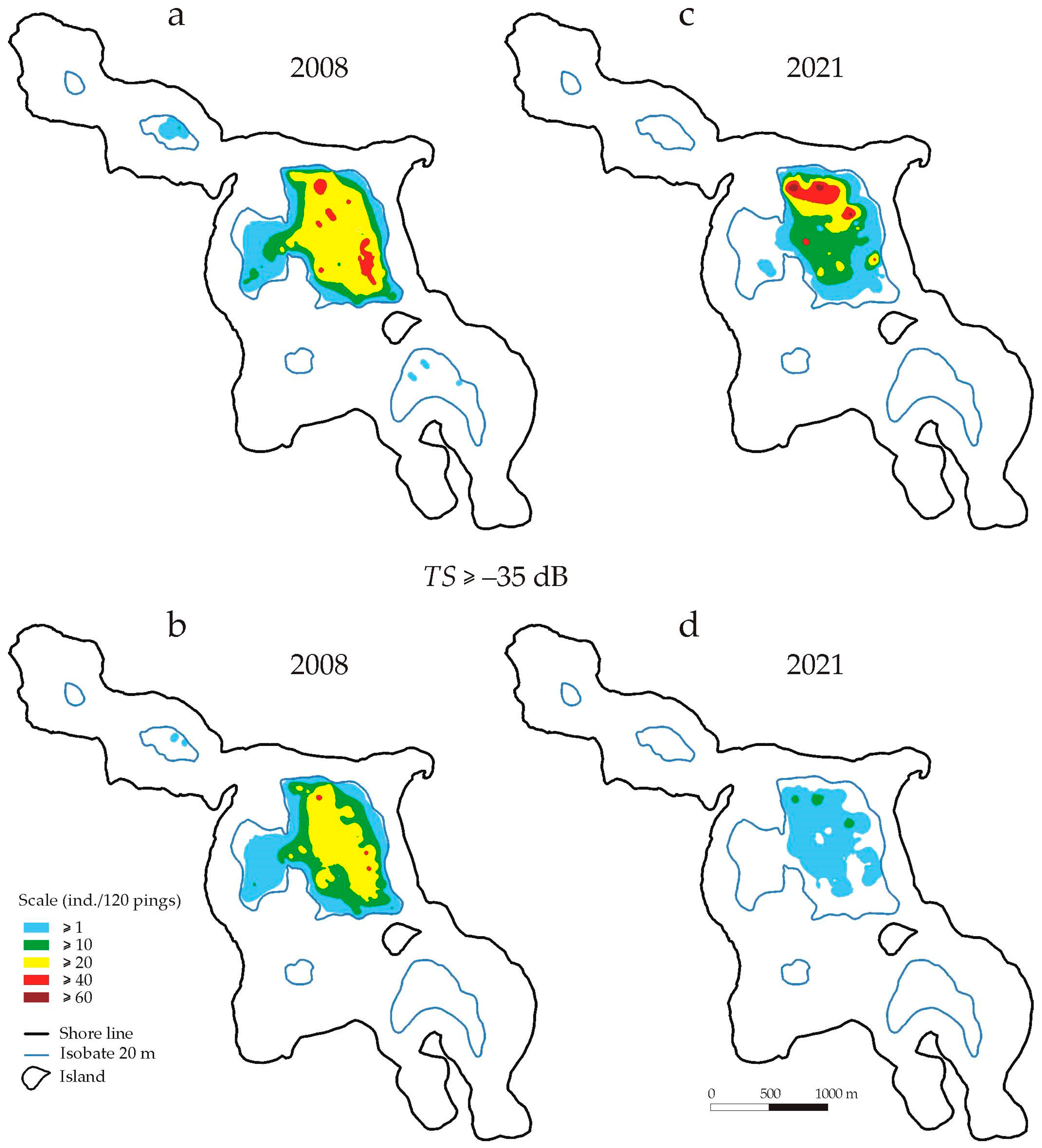
Based on the target strength distribution in the depth gradient (shown in
Figure 3), water layers were selected in which mapping of the distribution of the total number of fish and the number of fish with
TS > −35 dB, which was recorded on route sections with a length of 120 pings. According to Equation (1), the
TLF in 2021 is assumed to be >23.3 cm. Two layers of 20–22 m and 22–24 m were taken into account. In 2021, the presence of fish was still recorded in these layers; although, compared to 2008, a clear decrease in the number of fish larger with
TS > −35 dB was observed.
Mapping showed that in 2008, the area in the central part of the lake where fish were recorded (
n ≥ 1 individuals/120 pings) covered approx. 122 ha (
Figure 4a,
Table 2). This area was almost equal to the area surrounded by the 20 m isobath in the central part of the lake (130 ha) and constituted 63% of the total bottom area surrounded by the 20 m isobath (182 ha). At this depth, in the north-western and south-eastern parts of the lake, fish appeared sporadically. However, no fish with
TS > −35 dB were observed in these places (
Figure 4c). In the central part, they were still recorded on 89% of the area available in this part of the lake and at a density of 10 ≤
n < 20 ind./120 pings in a similar area (72 ha) as the total number of fish (83 ha). In 2021, the area of fish occurrence (
n ≥ 1 ind./120 pings) at a depth of 20–22 m was much smaller (by 26%) than in 2008 (
Figure 4c,
Table 2). The area where a greater number of fish was recorded (n > 20) covered practically only the deepest parts of the water column—only 15% of the area with a depth of at least 20 m (
Table 2). Fish with
TS > −35 dB (
TLF > 16.6 cm) were occasionally found here. No fish were observed in the north-western and south-eastern parts of the lake (
Figure 4d).
In 2008, in a layer 22–24 m deep, fish were found (
n ≥ 1 ind./120 pings) only in the central and northern parts of the lake. They occurred in an area (108.6 ha) covering 75% of the bottom area surrounded by a 22 m isobath. In the central part, they were found in 97% of the available area (
Figure 5a). A higher density of fish (10 <
n ≤ 20) was recorded only in the central part—in 65% of the area available in this part of the lake. Densities greater than
n > 40 ind./120 pings were observed in 37% of the available area. Fish with
TS > −35 dB were found in an area of 104.6 ha, mainly in the central part of the lake (
Figure 5b), and in slightly higher densities (
n > 20 pieces/120 ping) in 48% of the area available in this part of the lake.
In 2021, the area of fish occurrence at a depth of 22–24 m (
n ≥ 1 ind./120 pings) was 37% smaller than in 2008 (
Table 2). However, the area where fish occurred in larger numbers (
n 10 ≥ ind./120 pulses) decreased by as much as 66%. Fish with
TS > −35 dB (
TLF > 16.6 cm) were found in an area representing 27% of the available area in this part of the lake (
Figure 5d). It was 71% lower than in 2008. Slightly higher densities of these fish (
n > 10) were recorded in an area of only 0.1 ha (
Figure 5d,
Table 2).
Acoustic studies of Lake Dejguny showed significant changes in the distribution of TS fish communities throughout the lake and in the vertical profile. However, mapping allowed us to demonstrate a reduction in the space available for fish in waters below 24 m deep (habitat loss).
Size is the main structural feature in fish assemblages. Size strongly influences organismal movement, predation, growth, mortality, and reproduction of fish [
33]. It is well documented that most ecological and physiological processes are strongly dependent on body size [
34]. Barange et al. [
35] confirmed that
TS information in studies of the structure and dynamics of fish populations can be effective in the case of low-density, multi-species assemblages. Emmerlich et al. [
36] showed that non-taxonomic variables describing size-structured communities may be consistent with descriptors of lake morphometry, lake productivity (expressed by total phosphorus and chlorophyll a concentration), lake use intensity, and the taxonomic and functional composition of fish communities. Because the results presented in this study were obtained using the same method (same equipment, and same echogram analysis and mapping methods), the observed changes in the
TS structure and the spatial distribution of fish in Lake Dejguny are the result of structural changes in the lake ecosystem.
This conclusion is confirmed by the observed changes in the distribution of oxygen in the lake. In October 2021, in the lower parts of the lake, below 23 m depth, the concentration of dissolved oxygen in the water dropped below 2.5 mg O
2 ∙ L
−1, which is over 10 m shallower than in October 2008 (
Figure 3). This value limited the occurrence of fish in the lake.
Conducting a series of analogous studies on many lakes should enable the development of a simple indicator assessing changes in the ecological state. It seems that this future indicator could be based on the Large Fish Index (LAFI), which is used in marine ecology research. LAFI is based on the number of large fish as a percentage of all acoustically recorded fish echoes. LAFI is sensitive to the effects of fishing and relatively insensitive to environmental variability. However, it can be easily linked to a specific ecological quality status based on a reference period [
29]. Therefore, until the possible calibration of this method of assessing changes in the ecological state over time, it is necessary to determine the value of the indicator on two dates (the initial one and the one being compared).
Therefore, it was assumed that:
- -
The target strength TS distribution sufficiently describes precisely the changes in the size spectrum of the fish community;
- -
An indicator based on the essence of the Large Fish Index can effectively assess changes in ecological status by comparing values at the beginning and end of a specific period;
- -
Percentage share (%), calculated as the number of large fish divided by the number of smaller fish, can be as effective as the percentage of biomass of fish species or fish assortment, used in LIF-EN and LAFI, to assess the structure of ichthyofauna.
The latter assumption was based on Murry & Farrell’s statement that the distribution of the number
N as a function of unit length
L can determine the spectrum of community size [
37].
In this study, these proportions (
IND) of the number of fish with
TS > −38 dB (i.e., when
TLF 2021 > 16.6 cm) were determined in relation to the number of fish with −47 dB <
TS < −41 dB, expressed as
The
IND2008 value was 0.404,
IND2021—0.154.
IND2021 was therefore 2.6 times smaller than
IND2008. The index value for the 2008 data was also higher than the LAFI = 0.3 value, which corresponded to the range of values in the period 1925–1983 in the North Sea, when most of the exploited stocks were above the precautionary reference limit for spawning stock biomass [
14]. Therefore, the conducted research does not exclude the possibility of conducting analyses to develop an indicator based on acoustic data.
To sum up, hydroacoustic studies carried out in Lake Dejguny (analysis of TS distribution and maps of fish distribution in water layers) indicate that they can be a complementary method to the intercalibrated national method for assessing the ecological state of lakes based on fish. The LFI-EN method is based on determining the weight shares (%) of bream (Abramis Brama L.), silver bream (Abramis bjoerkna L.), roach (Rutilus rutilus L.), bleak (Alburnus alburnus L.), and ruffe (Gymnocephalus cernua L.) (which show an increase with increasing environmental pressure indicators) and the weight share of tench (Tinca tinca L.), rudd (Scardinius erythrophthalmus L.), and perch (Perca fluviatilis L.) (which show a decrease with increasing environmental pressure indicators). Therefore, information about the TS structure of fish obtained using acoustic methods is completely unsuitable for carrying out assessment using the LFI-EN method. However, acoustic tests allow us to indicate changes in the size structure of fish. It can, therefore, be concluded that carrying out acoustic tests (as preliminary tests) may indicate the need to carry out an assessment using the LFI-EN fish index, or the lack of such a need.


