Index-Based Groundwater Quality Assessment of Nestos River Deltaic Aquifer System, Northeastern Greece

Abstract

The Nestos River delta is one of the most important and sensitive basins in Greece and Europe due to its ecosystem functions, combining intensive agricultural production with low-enthalpy geothermal energy and important ecotopes. High water quality is of paramount importance to the sustainability of the system. Systematic and continuous assessment of water quality needs to be carried out in a way that is easy and quick for decision makers and non-expert societal partners to comprehend. In this way, decisions may be made more rapidly, and involved water users may be sensitized to rational water use. To this end, this paper presents the assessment of groundwater quality in the Nestos River’s western delta with the use of Poseidon (PoS), a versatile, index-based method. Groundwater samples collected from 24 and 22 wells tapping the unconfined and the confined aquifers, respectively, in four time periods (May and October 2019 and 2020) were analyzed. Using the PoS index, groundwater samples were classified according to their quality status, highlighting the parameters driving quality degradation issues, thus assisting water managers in obtaining an overview of quality status and evolution through datasets that were often large. PoS index is applied in the study area for the first time and provides a groundwater quality assessment through a unique score representative of the overall water quality status regardless of processes (anthropogenic or natural) or any kind of pressures.

1. Introduction

Groundwater quality assessment is often founded on traditional methods based solely on the comparison of analytical parametric values or calculation of molar ratios [1,2,3]. These methods can be very helpful, but, in most cases, they do not provide a convenient supervisory correlation between the examined samples, whilst identification of trends often proves to be unclear.

A variety of graphical techniques (those of Piper, Durov, Wilcox, etc., and diagrams) that have been proposed in the literature are also widely used [4,5,6] along with numerous synthetic ratios such as the sodium adsorption ratio and the Revelle factor [7]. Multivariate statistical techniques, such as correlation analysis, clustering analysis (CA), factor analysis/principle component analysis (FA/PCA), etc., are widely applied to understand processes, correlations, and hydrogeochemical evolution trends in groundwater systems. Correlation analysis is carried out as a bivariate statistic to determine the mutual relationships and strength of association between pairs of variables through calculation of the linear Pearson’s correlation coefficient [8]. Cluster analysis is a multivariate method based on the categories of data according to predetermined selection criteria. In this method, data are placed in clusters that indicate high internal (within-cluster) homogeneity and high external (between-cluster) heterogeneity [9]. Statistical methods such as those mentioned resolve issues relating to the identification of correlation and clustering of parameters that may be linked to the hydrogeochemical identity of the studied water samples, whilst they may also prove invaluable in deciphering or, at least, proving the hydrochemical types identified with the use of parametric ratios and graphical representation in one of the numerous available diagrams. Isotopic analyses are a valuable tool that often provide a higher resolution with regards to water origin where other conventional methods, such as those discussed above, fail.

Even though, in most of cases, the appropriate combination of some or all of the above discussed methods may provide definitive results with regards to groundwater origin, dominant evolution mechanisms, and spatiotemporal trends [10,11,12], they are not easy to be comprehend for non-experts, and they fail to provide an on-the-fly overview of the quality status to decision makers. Undoubtedly, reliable and objective assessments need to be based on systematic monitoring and consideration of a broad spectrum of parameters, which in several cases can be puzzling to decision makers. On the other hand, methods such as those mentioned above do not often allow for direct comparisons between different systems exposed to variable pressures and characterized by diverse hydrogeochemical settings and hydrodynamic evolution mechanisms.

Index-based methods may provide an alternative to overcome this shortfall, as they offer a quick assessment of groundwater quality in the form of a simple arithmetic value. They were introduced in the 1960s and were already adopted as official tools by water resource monitoring agencies in the 1970s [13]. Depending on the method, a different number of physicochemical and, in some cases, microbiological parameters are assessed, and quality evaluation is usually based on the criteria set for a particular use. Their usability, amongst others, relies on the fact that they reduce the inherent complexity of water sample analysis to a simple arithmetic value which is easy to comprehend. Over 30 such methods have been reported by other researchers [14]; these methods use a widely varying number of parameters ranging from 3 to 72. Often, index-based approaches adopt specific water-use quality standards, thereby potentially masking the overall quality attributes of a sample. Whilst a review of the developed index-based methods is not within the scope of this paper, it is worth noting the USA and the Canadian Water Quality Index (CWQI) methods as milestones and amongst the most well-known and widely used ones. A thorough benchmark study amongst these methods concluded that the CWQI yields more stringent classifications, i.e., provides a more end use-sensitive result, compared to the USA methods [15]. As is also the case with the USA methods, the CWQI considers as baseline for its assessments the potability criteria and classifies assessed water samples in five grades on a scale of 0–100, with 0 representing the worst and 100 the best water quality [16]. The number of parameters that are suggested for use in the assessment varies from 8 to 20; however, less than 8 or more than 20 may be used [17]. Calculation of the CWQI is based on three factors, namely, the scope, which represents the percentage of parameters that do not meet the quality standards at least once over the considered period of evaluation; the frequency, which refers to the percentage of individual tests failing the standards; and the amplitude, which represents the amount by which the failed test values do not meet the standards [16].

A relatively new method, the Poseidon index (PoS), is an alternative, versatile, index-based method for the assessment and classification of water samples [10]. The concept of the method relies on the fact that each water sample has an environmental quality status that, however, is shaped as a result of geogenic and anthropogenic factors and, thus, may not be uniquely associated to specific maximum admissible concentrations assumed for a particular use. Therefore, the method seeks to examine and assess the environmental quality status of a water sample, accounting for the origin of each of the compounds that synthesizes it. Any number of parameters may be considered in the assessment, and each of them is weighted against its toxicity classification as this is referenced in the key document of ATSDR [18]. Specific use standards are being considered, and, normally, these are the most stringent potability standards and, therefore, are environmentally sensitive. However, these standards only serve as a basis for initiating the assessment, and by no means are they related to the actual classification of the water, as explained in the following paragraphs. Classification is based on a scale of 0 to over 2400, where 0 corresponds to no/minimum degradation, and over 2400 corresponds to a severe degradation of the water’s quality. This scale is organized in six color-coded classes and corresponding subclasses (a, b, c) for classes two to five, thus enabling a more detailed categorization of assessed qualities. Moreover, the method allows for the identification of the parameters that control the quality assessment, helping to trace and correlate quality issues to their origin.

2. Poseidon (PoS) Index

PoS is a relatively new index-based operational method developed to address the aforementioned issues in assessing groundwater quality. PoS differs from other methods in that it provides a general operational comparison between different sampling points, irrespective of the measured parameters, sampling times, and time deviations (comparison between different points in different catchment areas and sampling periods) [3,10]. It allows temporal comparisons between different sampling periods in the same basin and assessments between different groundwater systems in the same or different basins, under different pressures, and controlled by different mechanisms [11].

Compared to other quality assessment methods that are proposed in the literature, PoS presents some key differences [10]. The main differences are [19]: (a) the calculated PoS index does not change with the parameters used (number and nature) and (b) other methods focus either on (i) specific objectives (e.g., sea water intrusion, chemical status), (ii) specific processes (e.g., origin of water), or, finally, (iii) end use-related characterization (e.g., quality of drinking or irrigation water).

PoS provides quality assessment through a unique score representative of the overall water quality status regardless of processes (anthropogenic or natural), objectives, and characterization, as described in the foundation paper of the index [10], and has been successfully applied in a series of cases of complex systems’ quality assessments [12,19,20], in conjunction with statistical or more conventional hydrochemical analysis methods, or in comparatively assessing water quality characteristics amongst vastly different hydrogeological basins [11].

It should be noted that PoS index not only provides the environmental quality status of a groundwater sample but also identifies the chemical parameter(s) which causes the deviation from a “good” environmental status, thus narrowing down the likely sources of the problem. Thus, the proposed approach directly relates the outcome of the assessment to the concentrations of selected chemical parameters which may have adverse effects on health and the environment. PoS serves, therefore, as a robust and fully comprehensive means of reducing the inherent complexity in hydrochemical data sets to an easy-to-understand quality index, and, as such, it does not reflect on end user or different types of water regulatory frameworks. The following table,

Table 1. Parameters for calculating the PoS index and classification of these parameters based on their toxicity, individual score, and weighting factor.

Toxic Class	Substances	Points	P-Class	Partial Score (PS)	Weighting Factor (Wf)
1	As	1	VI	10	0.19
2	Pb	10	V	8	0.16
	Cd	10	V	8	0.16
3	NH4	100	IV	5	0.10
	NO2	100	IV	5	0.10
4	NO3	1000	III	3	0.06
	B	5000	II	1.5	0.03
	Cu	5000	II	1.5	0.03
	Mn	5000	II	1.5	0.03
	Ca	50,000	I	1	0.02
	Cl	50,000	I	1	0.02
	Fe	50,000	I	1	0.02
	K	50,000	I	1	0.02
	Mg	50,000	I	1	0.02
	Na	50,000	I	1	0.02
	SO4	50,000	I	1	0.02
	EC	50,000	I	1	0.02

, provides the parameters used in this paper for calculating the PoS index and classifies these parameters based on their toxicity, individual score, and weighting factor.

The calculation of the PoS index is based on the use of the most usual inorganic substances commonly found in groundwater. These substances may originate from a variety of sources such as agriculture, sea intrusion, rock weathering, industry, and household waste. The method provides a wide list of parameters that, ideally, should all be considered. However, in several cases, not all listed parameters are available, whilst, in other cases, quality evaluation focuses on a particular objective to which not all of the listed parameters are relevant. Each parameter selected is classified according to its overall (synergistic/additive) health and environmental impact. The toxicity of each agent to humans plays a key role in this; their classification is based on the “Priority List of Hazardous Substances” [18] but was further elaborated by toxicological data obtained from various published sources [21,22] and well-established international organizations, such as the WHO [23], in order to ensure a comprehensive examination of critical aspects of water quality.

The classification of each parameter is based on its toxicity; this is also a key difference from most index-based methods, and the main objective is the relative comparison between concentrations of the selected parameters for the purposes of the PoS index. Based on the above, the selected parameters are classified, accordingly, into six categories (P-class), as shown in Table 1.

Depending on the overall incidence of toxicity in humans, a partial score (PS) is assigned to each P-class which reflects the degree of overall toxicity for humans. The reference values used were based on those applied in references [10,11,12]. The individual PS score follows an exponential approach, but the scale between them is carefully chosen to differentiate between the recognized P-class classes without overlapping the lower ones.

The weighting factor/Wf for each parameter is subsequently calculated, based on the partial score, according to Equation (1):

$$\mathrm{Wfi}=\frac{PSi}{\Sigma PSi}$$

(1)

The partial scores were selected through a procedure using a trial-and-error approach. The main purpose of this procedure was to obtain the best possible results so that the weighting factor (Wf) of a parameter belonging to the P-class (V) will be a rank higher than that of a parameter belonging to the IV class. Thus, for Cd or Pb, the Wf was calculated at 0.15, while for Cu or Mn, the Wf was calculated at 0.03. This is because, while the differences between categories I and II (non-toxic) and V and VI (highly and severely toxic), in terms of overall environmental impact, are insignificant, the effects between non-toxic and toxic categories must be clearly distinguished.

The reliability of the final weights was confirmed by multivariate techniques (object analysis) by calculating Cronbach’s alpha (a) coefficient, which represents the internal consistency of the values considered [24]. The coefficient (a) ranging between 0 and 1 and the highest values indicate greater consistency between the examined values, with a historical reference point of acceptable values greater than 0.7. The lower the value in column points, the higher the P-class. The points in the following table, Table 1, are based on the value of toxicity [18].

The impact of each parameter on the overall quality assessment of each sample is attributed through each quality contribution factors (Qf). The quality contribution factors are derived from the following Equation (2):

$$\mathrm{Qfi}=[\frac{(Ci\ast Wi)}{MACi}]\times {10}^3$$

(2)

where Qfi is the quality contribution factor of the parameter i; Ci is the concentration of the parameter i (same units as the parameter); Wi is the weighting factor of the ith parameter; and MACi is the maximum parametric value of the ith parameter (the maximum acceptable concentration specified in Directive 2020/2184 EC [25] for water intended for human consumption; this serves only as a reference basis and does not actually interfere in the final quality characterization).

The final PoS index is obtained by summing all the individual Qfis according to the following equation, Equation (3). The PoS index is a dimensionless number that can be used for the qualitative evaluation of a sample.

PoS = Σ Qfi

(3)

The contribution of each parameter to the overall qualitative status of the sample, as a percentage, is derived from the Qfi calculation ratio. The prevailing control parameters are those with a contribution rate greater than 20% [10].

The PoS index score calculated for each sample classifies it into a category according to a classification system, based on a six-base color palette, according to the following table,

Table 2. Presentation of the PoS indicator (range of categories, subcategories, and qualitative degradation color rendering).

PoS Class	Range	Min	Max	Subclass Range	a		b		c		Quality Degradation Level	Color
1	a ≤ t	0	150	-	<t						None–Low
2	t < a < 2t	150	300	50	150	200	200	250	250	300	Low
3	2t < a < 4t	300	600	100	300	400	400	500	500	600	Moderate
4	4t < a < 8t	600	1200	200	600	800	800	1000	1000	1200	High
5	8t < a < 16t	1200	2400	400	1200	1600	1600	2000	2000	2400	Very High
6	a > 16t	2400	-	-	-						Severe

. This is carried out so that the calculated PoS index score, which is simply a number, is represented by a color to understand and interpret each sample’s score. In the PoS index, every one of the six classes ranges from 0 to t, from t to 2t, from 2t to 3t, etc. Classes 2-5 are divided into three subclasses (a, b and c), offering a better resolution between the tested samples. Each of the main categories (except the first and last) is divided into three equally wide subcategories, on a progressively increasing scale, in order to ensure better representativeness and differentiation of the results. Categories 1 and 6 need not be further differentiated as they represent boundary quality conditions. As a result, these classes can be considered as critical limits of higher and lower groundwater quality, respectively. The upper and lower limits of each one of the three subclasses are tabulated in Table 2.

The procedure for calculating a value corresponding to the threshold of the PoS index was carried out based on a reference sample and with concentrations reflecting the average typical concentrations expected in natural groundwater for the selected parameters. The value used to define the classes and subcategories of the PoS index is 150 [1] and can be used as the fundamental constant step for the classification of the PoS index, regardless of the parameters involved at one time. Its calculation was based on several trial-and-error tests which were performed with various combinations of parameters and which produced similar values. The higher the class of the PoS index, the lower the overall environmental quality of the water, expressed by the color hue of the PoS index.

The final stage of the process involves the evaluation through a comprehensive and simplified presentation which provides the key elements of the indicator. This process includes:

(i)

The main category of the PoS index (1 to 6) and its subcategory, if any;

(ii)

The dominant factor (or factors with a Qfi > 20%) which controls the quality status of the sample;

(iii)

A final unique color characterization, which makes the data visually clearer, followed by accurate information on the level of quality degradation.

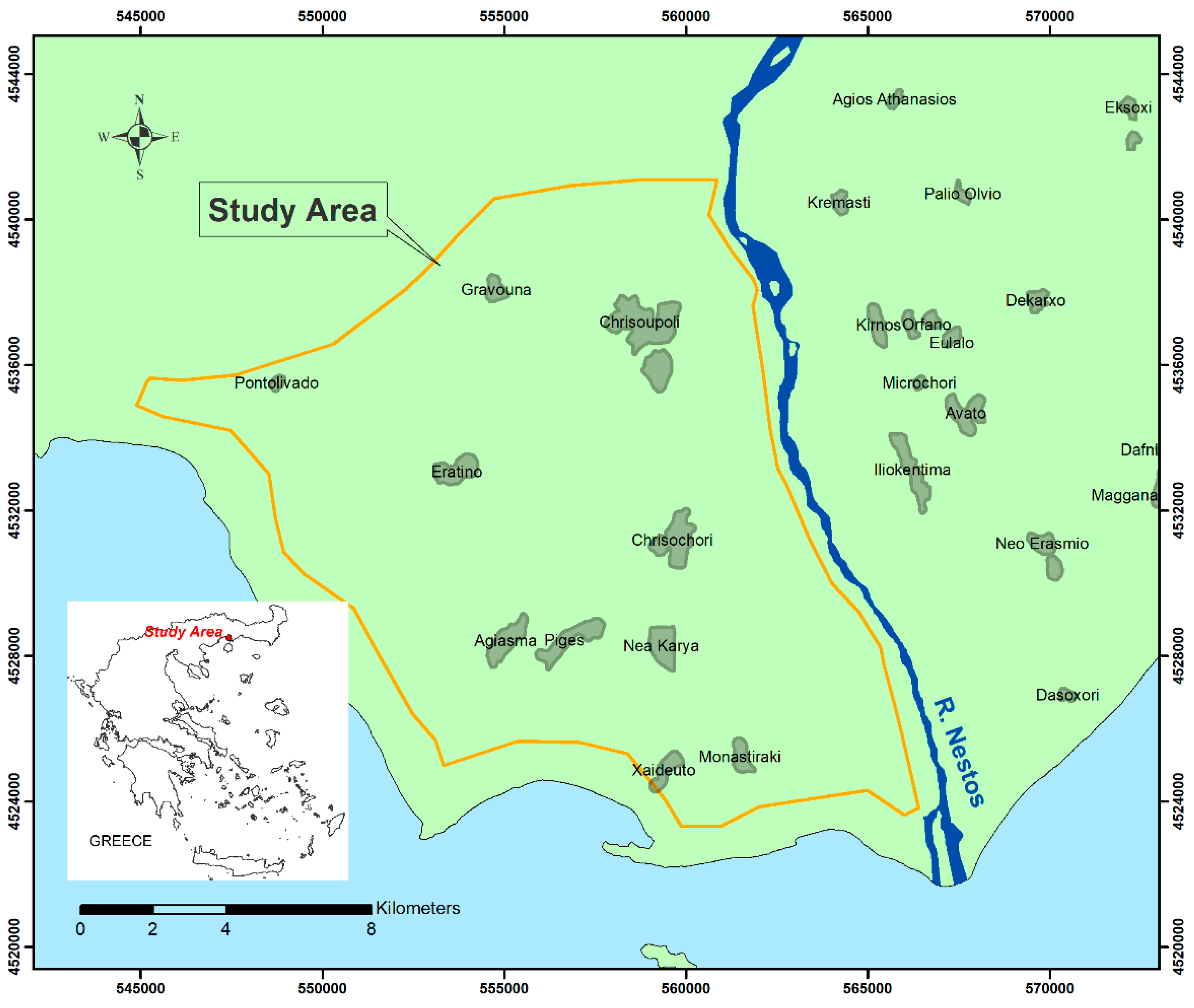
It is noted that the term “quality degradation” refers to a comparative characterization among the samples examined under the PoS index and, in no case, does it imply any specific characterization under the relevant legislation and/or international standards.

3. Case Study

The study area is located at the western part of the Nestos River delta (Figure 1) at the eastern coastal region of the Kavala Prefecture, Northeastern Greece. It is delineated by the Thracian Sea coastline to the south and west, the riverbed of the Nestos River to the east, and the Rhodope geological massif to the north, thus including the full length of the Nestos River along its deltaic plain. The river delta belongs to the National Park of Eastern Macedonia and Thrace, which was founded in the year 2008. In this section of the Nestos River delta, a great number of settlements are present. The river visibly splits the delta in almost two equal parts, expanding from the settlements of Nea Karvali to the west, up to Toxotes to the north, and Avdira to the east.

The deltaic plain slopes gently to the south with elevations ranging from +40 m at the northern margin to 0 ± 1 m at the southern end near the coastline. Limited-size morphological depressions are identified from north to south; these give rise to secluded seasonally filled stagnant water bodies (lakes or swamps). These features, and especially the marshes, were most distinguished in the early development phases of the delta and primarily owe their existence to residues of older secondary river courses or to mountain-zone currents.

In the whole study area (210.73 km²), agriculture is the dominant land use (over 77% landcover). A factor that contributes to deep percolation of groundwater recharge is flood irrigation, still practiced in many parts of the plain. An aftermath of this practice appears to be the prevention of seawater intrusion advancing into the coastal aquifer system; however, at the same time, this practice potentially affects groundwater quality by leaching pollutants originating from anthropogenic activities into the saturated zone. Finally, in recent years, shallow wells are mainly used for irrigation activities, while the use of deep wells is very limited and constrained to a short period of time [26].

4. Geo-Hydrological Setting

The deltaic region consists of Holocene sediments with an overall thickness of some tens of meters deposited mainly by the Nestos River and its substreams. These sediments are formed of alternate sand, clay, and silt layers, thus reflecting a broad spectrum of formational and depositional conditions. These conditions led to a very diverse geological domain. Moreover, the presence of organic clay in some spots is due to delta marshes.

The study area is part of the wider Nestos River delta. This delta is one of the wetlands of utmost significance in Greece and Europe because of the size and the diversity of its ecology. This ecosystem is part of the Ramsar Convention on Wetlands of International Importance and the Natura 2000 network and is a special protection area of the European Union Directive on the Conservation of Wild Birds. It is included in the National Park of Eastern Macedonia and Thrace, which extends from the Nestos River delta to the lakes of Vistonida and Ismarida. Overall, the Nestos River delta consists of various individual wetland ecosystems. The greatest and most significant of these are (in alphabetically order): The Agiasmos Lagoon, Bassova Lagoon, Chaidou Lagoon, Eratinos Lagoon, Keramoti Lagoon, Kokala Lagoon, Magana Lagoon, and Monastiraki Lagoon.

The minimum and maximum annual rainfalls for the period 1985–2019 were 227.30 mm and 968.20 mm, respectively. Taking into account that the mean annual precipitation value was 496.80 mm over this period, the mean annual volume of rainfall received in the study area was 104.69 × 10⁶ m³. The wettest and driest periods were November–December and July–September, respectively.

Two distinct units are present: (i) an unconfined aquifer and (ii) a confined aquifer system located in the Miocene sediment series. The former is primary recharged directly by precipitation, through percolation of the Nestos riverbed, and by lateral crossflows from the karst system located to the northern margin of the deltaic system. Lateral inflows contribute greatly to the recharge of the Miocene series aquifers. The unconfined aquifer, which is formed in the Quaternary deposits, is characterized by minor hydraulic head fluctuations.

The confined aquifer system is situated in the porous media of the delta (mainly sands and gravel which alternates with clays in vertical as well as in horizontal directions, forming a series of superimposed aquifers). Hence, under the unconfined aquifer, a series of confined aquifers exist up to a depth of at least 150 m. In the series of confined aquifer units, some artesian ones have been documented; these start from a shallow depth of about 15 m. In the Keramoti area, similar artesian units have been identified to a depth of approximately 120 m.

5. Materials and Methods

In the framework of this study, in situ measurements of groundwater temperature, pH, and electrical conductivity were performed at a monitoring network consisting of 24 and 22 wells in the unconfined and the confined aquifers (Figure 2), respectively, in four time periods (May and October 2019 and 2020). The monitoring periods correspond to the end of the wet and the dry seasons (May and October, respectively), thus are deemed representative of the extreme hydrological conditions in the region that are expected to reflect on the maximum potential water quality differentiations within a year. Groundwater samples were also collected from this network over the same periods and analyzed at the ELOT EN ISO 17025:2017-accredited laboratory of the Soil and Water Resources Institute of the Hellenic Agricultural Organization, Sindos, Greece, for the determination of 16 physicochemical and chemical parameters used in the calculation of PoS index: electrical conductivity (EC), NH₄⁺, ΝO₃⁻, ΝO₂⁻, Cl⁻, Na⁺, Ca²⁺, Mg²⁺, Mn²⁺, SO₄²⁻, and the dissolved forms of As, Pb, Cd, Cu, Fe, and B (As_dis, Pb_dis, Cd_dis, Cu_dis, Fe_dis, and B_dis).

Samples were collected in 1 L polyethylene bottles thoroughly cleaned with mild glass detergent, subsequently washed with deionized water, and air-dried. Samples were collected from taps or valves at the wellhead of each sampling point following operation of the pump for 5 to 10 min in order to ensure stagnant water from the pump mains was discharged and a representative groundwater sample was collected. A visual check of turbidity, and stabilization of the pH and EC values measured at the discharged water preceded sample collection, following which, sampling bottles were washed twice with discharged water, filled to the top, tapped, capped, and registered in dedicated sampling logs. In order to speed up field operations, no in situ filtration or chemical preservation was performed. Samples were transported to the laboratory facilities on the same day of sampling and cooled in thermally insulated containers with ice packs. At the laboratory facilities, samples were immediately filtered and stored in refrigerators at 4 °C. The fraction of the sample used for heavy metal determinations was acidified with ultra-pure HNO₃^- to pH < 2 [27]. Determinations were concluded within 2 days of collection for the major ions and EC and less than 10 days for the heavy metals. A set of counter samples was preserved for a period of a month as reference in case odd results dictated repetition of determinations.

Electrical conductivity was measured by a CRISON GLP 32 Conductimeter according to the ELOT EN 27888:1993 method [28]. Potentiometric measurement of alkalinity, carbonates, and bicarbonates was carried out using volumetric determination, according to the ELOT EN ISO 9963-1:1996 method [29]. Nitrates, nitrites, and ammonium were determined colorimetrically using a Perkin Elmer Lambda 35 UV/VIS spectrophotometer according to Standard Methods for the Examination of Water and Wastewater Handbook, APHA, 23rd edition [27], while boron was also determined colorimetrically using a Perkin Elmer Lambda 35 UV/VIS spectrophotometer according to Standard Methods for the Examination of Water and Wastewater, 2017, 1-43: “Sample Storage and Preservation and Methods of Soil Analysis, Part 3: Chemical Methods”, 1996, and Chapter 21, “Azomethine-Hydrogen Method” [30]. Cl^- was determined by the Mohr titration method [31]. Sodium was determined by Sherwood M410 Flame Photometer according to the ISO 9964-3:1993 method [32]. Calcium and magnesium were determined with a Perkin Elmer AAnalyst 700 Atomic Absorption Spectrometer according to Standard Methods for the Examination of Water and Wastewater, APHA, 3500, B, 23rd edition [27]. Trace elements and heavy metals were measured with a Perkin Elmer AAnalyst 700 Graphite Furnace Atomic Absorption Spectrometer according to the ELOT EN ISO 15586:2003 method [33], while mercury was determined with hydride generation atomic absorption spectrophotometry (HGAAS) [34].

Based on the results of the laboratory determinations, only negligible differences were noted between the two wet (May) and the two dry (October) sampling periods. On the contrary, as expected, changes were apparent between the dry and the wet periods. Hence, individual analysis and presentation of the results per sampling period would not add to the scope of the work, which comprises the identification and presentation of spatiotemporal variations in groundwater quality, focusing on possible discretization between the unconfined and the confined aquifers. Analysis of the results is, therefore, presented in the meaningful pattern of averaged values for the two wet (May 2019 and 2020) and the two dry (October 2019 and 2020) periods, as tabulated in

Table 3. Analytical results of groundwater determinations for unconfined aquifer (average values for May 2019 and 2020).

Well Code	Asdis	Pbdis	Cddis	NH4+	NO2−	NO3−	Bdis	Cudis	Mndis	Ca2+	Cl−	Fedis	Mg2+	Na+	SO42−	EC
	μg/L	μg/L	μg/L	mg/L	mg/L	mg/L	mg/L	μg/L	μg/L	mg/L	mg/L	μg/L	mg/L	mg/L	mg/L	μS/cm
25	1.00	<LOD	<LOD	<LOD	0.04	7.36	0.04	<LOD	844.70	84.40	10.50	59.18	11.88	9.05	22.58	546
26	25.35	<LOD	0.19	0.79	0.07	17.84	<LOD	<LOD	1016.10	76.48	14.88	6.27	16.53	16.76	45.04	549.5
27	6.43	<LOD	0.31	0.90	<LOD	<LOD	<LOD	<LOD	939.68	114.30	10.91	73.14	16.33	22.35	78.04	732.5
28	8.00	<LOD	0.21	0.06	0.41	17.34	0.14	<LOD	784.54	132.38	57.08	8.42	39.50	75.88	122.65	1118.5
29	<LOD	<LOD	<LOD	0.30	1.24	11.86	0.08	<LOD	791.35	81.08	13.28	156.35	16.38	23.78	17.85	635
30	<LOD	<LOD	<LOD	<LOD	0.25	5.33	0.11	<LOD	1262.35	80.05	13.73	128.32	23.60	38.81	59.76	722.5
31	<LOD	<LOD	0.46	0.07	0.23	8.21	<LOD	<LOD	1347.75	88.45	9.87	13.80	11.80	11.52	32.40	645.5
32	1.34	<LOD	0.23	0.08	0.25	9.57	<LOD	<LOD	797.26	81.23	7.64	6.48	8.90	8.16	3.52	422
33	<LOD	4.28	<LOD	4.90	<LOD	30.83	<LOD	<LOD	20.77	85.46	95.05	302.70	11.63	81.98	71.27	837
34	<LOD	<LOD	<LOD	0.11	<LOD	37.27	<LOD	<LOD	25.46	126.00	55.60	15.42	10.25	34.48	77.76	848
35	6.58	<LOD	0.24	4.11	0.02	<LOD	0.28	<LOD	760.88	64.65	126.29	26.76	42.13	127.62	5.97	1086.5
36	7.08	<LOD	<LOD	0.52	0.08	5.64	<LOD	<LOD	1394.25	95.28	33.44	32.72	18.58	28.72	65.04	717
37	7.98	<LOD	0.44	<LOD	0.43	13.17	<LOD	<LOD	369.54	55.85	6.56	<LOD	6.80	7.06	<LOD	335
38	8.99	<LOD	<LOD	0.34	0.02	<LOD	0.05	<LOD	1346.00	100.63	26.01	27.84	20.93	49.57	78.04	749
39	4.45	<LOD	<LOD	<LOD	<LOD	<LOD	<LOD	<LOD	22.67	106.73	399.11	19.30	29.10	182.93	18.88	1728
40	16.88	<LOD	<LOD	2.89	<LOD	1.22	0.39	<LOD	964.50	84.15	268.38	42.18	27.50	364.82	<LOD	2310
41	6.23	<LOD	0.19	5.30	<LOD	5.11	0.52	12.63	199.86	40.49	60.82	769.90	15.20	155.56	<LOD	986.5
42	45.58	<LOD	<LOD	1.66	0.02	<LOD	<LOD	<LOD	2345.60	67.48	6.89	102.02	8.48	10.68	<LOD	416
43	10.98	<LOD	0.31	1.37	<LOD	<LOD	<LOD	<LOD	1277.30	73.33	9.19	135.10	11.78	9.44	<LOD	454
44	3.38	<LOD	0.27	0.67	<LOD	<LOD	0.10	<LOD	981.00	86.83	25.14	82.75	19.48	65.79	74.67	860.5
45	10.09	<LOD	<LOD	0.78	0.06	12.50	0.42	<LOD	966.90	105.40	55.60	12.13	38.45	134.16	132.18	1206
46	4.94	<LOD	0.19	0.61	0.26	12.02	0.07	<LOD	1314.25	116.45	24.99	22.30	30.85	43.48	109.64	816

Note: LOD: Limit Of detection.

,

Table 4. Analytical results of groundwater determinations for unconfined aquifer (average values for October 2019 and 2020).

Well Code	Asdis	Pbdis	Cddis	NH4+	NO2−	NO3−	Bdis	Cudis	Mndis	Ca2+	Cl−	Fedis	Mg2+	Na+	SO42−	EC
	μg/L	μg/L	μg/L	mg/L	mg/L	mg/L	mg/L	μg/L	μg/L	mg/L	mg/L	μg/L	mg/L	mg/L	mg/L	μS/cm
25	5.11	<LOD	<LOD	0.17	<LOD	5.09	<LOD	<LOD	266.00	97.63	9.31	11.68	11.30	9.10	26.31	553
26	23.00	<LOD	<LOD	0.96	0.06	14.76	0.08	<LOD	387.50	79.48	13.52	9.58	14.48	15.21	44.85	571.5
27	6.21	<LOD	<LOD	0.74	<LOD	<LOD	<LOD	<LOD	709.50	109.60	9.25	15.39	13.95	17.29	51.22	653
28	12.74	<LOD	<LOD	0.07	0.15	34.41	0.13	<LOD	315.76	80.43	36.55	4.85	22.25	66.11	87.22	884
29	4.37	<LOD	<LOD	0.38	0.03	6.57	0.05	<LOD	263.46	78.58	10.56	14.82	12.53	20.08	24.04	541.5
30	2.94	<LOD	<LOD	0.14	0.13	11.21	0.10	<LOD	896.75	98.95	14.62	29.91	24.65	41.75	64.67	756
31	3.05	<LOD	<LOD	<LOD	0.31	12.62	<LOD	<LOD	712.00	121.25	10.59	11.00	10.90	10.39	42.13	673.5
32	2.29	<LOD	<LOD	0.12	0.20	7.29	<LOD	<LOD	300.06	89.58	11.56	8.12	8.88	8.90	32.49	516
33	1.73	<LOD	<LOD	10.12	0.06	<LOD	0.04	<LOD	17.72	33.64	85.81	201.24	12.88	57.43	83.40	728
34	3.10	<LOD	0.27	<LOD	<LOD	31.82	<LOD	<LOD	7.00	141.23	39.58	30.42	9.38	37.85	65.95	830
35	8.39	<LOD	<LOD	1.28	<LOD	<LOD	0.74	<LOD	403.88	73.53	22.51	38.67	31.90	43.49	68.04	704.5
36	2.84	<LOD	<LOD	0.37	0.06	6.14	<LOD	<LOD	466.75	100.75	11.22	10.65	18.90	29.46	65.40	675.5
37	9.91	<LOD	<LOD	0.17	<LOD	6.30	<LOD	<LOD	138.53	46.85	5.37	35.85	5.65	6.87	8.31	317
38	9.19	<LOD	<LOD	0.34	<LOD	<LOD	0.10	<LOD	848.13	91.50	15.01	10.73	22.10	86.87	67.90	771
39	4.38	<LOD	<LOD	<LOD	<LOD	<LOD	0.09	<LOD	9.87	154.43	261.27	32.97	41.15	268.76	38.67	2295
40	21.89	<LOD	<LOD	2.04	0.02	3.11	0.27	<LOD	404.76	64.55	268.38	27.87	20.28	238.58	5.97	1617
41	8.20	<LOD	<LOD	2.92	<LOD	1.15	0.28	<LOD	180.81	48.78	26.12	187.57	11.88	66.45	<LOD	626.5
42	23.26	<LOD	<LOD	1.41	<LOD	<LOD	0.06	<LOD	732.31	63.60	6.68	119.71	7.85	11.11	<LOD	390.5
43	8.12	<LOD	<LOD	1.60	<LOD	<LOD	0.04	<LOD	500.75	73.88	5.72	49.50	11.93	1.00	<LOD	469
44	4.14	<LOD	<LOD	0.77	<LOD	<LOD	0.14	<LOD	939.80	110.18	18.86	65.01	21.85	72.49	74.95	892.5
45	6.95	<LOD	<LOD	0.11	<LOD	6.89	0.46	<LOD	313.25	100.58	130.79	18.01	38.83	132.40	97.59	1235
46	4.03	<LOD	<LOD	0.23	0.09	16.18	0.04	<LOD	760.38	116.45	19.66	38.20	29.53	42.98	120.55	802.5

Note: LOD: Limit Of detection.

,

Table 5. Analytical results of groundwater determinations for confined aquifer (average values for May 2019 and 2020).

Well code	Asdis	Pbdis	Cddis	NH4+	NO2−	NO3-	Bdis	Cudis	Mndis	Ca2+	Cl−	Fedis	Mg2+	Na+	SO42−	EC
	μg/L	μg/L	μg/L	mg/L	mg/L	mg/L	mg/L	μg/L	μg/L	mg/L	mg/L	μg/L	mg/L	mg/L	mg/L	μS/cm
1	9.72	<LOD	<LOD	0.12	<LOD	<LOD	0.50	<LOD	12.95	189.63	164.25	189.63	2.41	253.19	52.95	1234.5
2	99.03	<LOD	<LOD	2.84	<LOD	<LOD	0.20	<LOD	756.85	226.48	42.87	226.48	18.40	75.26	<LOD	741.5
3	4.80	<LOD	<LOD	0.77	<LOD	<LOD	0.16	<LOD	662.69	27.46	23.65	27.46	16.70	95.96	<LOD	705.0
4	1.40	<LOD	<LOD	0.50	<LOD	<LOD	<LOD	<LOD	650.76	49.07	52.98	49.07	10.55	36.59	2.79	637.0
5	15.34	<LOD	<LOD	0.75	<LOD	<LOD	<LOD	5.55	830.11	87.55	8.61	87.55	8.48	17.45	<LOD	412.0
6	71.51	<LOD	<LOD	1.90	<LOD	<LOD	0.10	<LOD	1346.95	129.01	8.45	129.01	17.55	46.30	<LOD	511.0
7	30.82	<LOD	<LOD	3.02	<LOD	<LOD	<LOD	<LOD	814.25	6.30	33.07	6.30	5.08	22.68	<LOD	553.5
8	0.97	<LOD	<LOD	0.09	<LOD	<LOD	0.12	<LOD	177.75	<LOD	7.47	<LOD	18.30	44.00	3.15	446.5
9	29.00	<LOD	<LOD	0.93	0.02	<LOD	0.18	<LOD	838.20	7.20	4.27	7.20	15.73	31.65	<LOD	436.5
10	19.03	<LOD	<LOD	0.09	<LOD	<LOD	0.52	<LOD	6.07	116.21	97.27	116.21	1.61	232.38	41.76	1035.0
11	14.72	<LOD	0.19	0.08	<LOD	<LOD	0.38	13.40	19.70	70.89	164.66	70.89	4.00	249.67	34.58	1172.5
12	3.56	<LOD	0.19	<LOD	<LOD	<LOD	0.16	<LOD	22.43	52.64	102.64	52.64	5.05	184.17	30.13	910.0
13	26.10	<LOD	<LOD	0.74	<LOD	<LOD	0.09	<LOD	481.71	373.85	46.75	373.85	10.43	48.93	2.70	700.5
14	38.68	<LOD	0.18	3.61	<LOD	1.07	0.18	<LOD	611.16	202.35	98.87	202.35	18.58	142.08	<LOD	987.5
15	95.70	<LOD	0.23	4.59	0.38	<LOD	0.57	<LOD	694.81	30.53	107.19	30.53	32.40	232.79	<LOD	1424.5
16	11.63	<LOD	0.20	0.21	<LOD	<LOD	0.39	<LOD	18.35	17.17	113.85	17.17	2.25	219.66	4.52	1004.0
17	3.98	<LOD	0.18	<LOD	0.03	5.99	<LOD	<LOD	465.93	6.41	13.13	6.41	11.03	18.20	9.40	435.0
18	14.62	<LOD	0.17	1.96	<LOD	<LOD	0.12	<LOD	782.25	307.94	7.20	307.94	9.60	35.84	3.79	464.5
19	2.72	<LOD	<LOD	0.17	<LOD	<LOD	0.41	<LOD	110.59	27.00	456.34	27.00	10.38	399.61	28.49	2127.5
20	16.19	<LOD	0.19	0.05	<LOD	<LOD	0.24	<LOD	27.00	21.69	24.50	21.69	1.14	160.95	<LOD	683.5
21	15.83	<LOD	0.42	<LOD	<LOD	<LOD	0.47	<LOD	19.03	<LOD	115.05	<LOD	2.08	222.89	15.95	1046.0
22	< LOD	<LOD	0.21	<LOD	<LOD	142.83	<LOD	<LOD	10.03	17.24	45.39	17.24	21.03	64.48	51.79	1166.0
23	9.72	<LOD	0.20	0.76	<LOD	55.69	<LOD	<LOD	40.81	55.26	133.55	55.26	14.08	121.27	71.49	1085.0
24	< LOD	<LOD	0.34	<LOD	0.02	28.72	0.19	<LOD	624.44	68.30	825.41	68.30	53.18	321.27	102.22	1915.5

Note: LOD: Limit Of detection.

and

Table 6. Analytical results of groundwater determinations for confined aquifer (average values for October 2019 and 2020).

Well Code	Asdis	Pbdis	Cddis	NH4+	NO2-	NO3-	Bdis	Cudis	Mndis	Ca2+	Cl-	Fedis	Mg2+	Na+	SO42-	EC
	μg/L	μg/L	μg/L	mg/L	mg/L	mg/L	mg/L	μg/l	μg/L	mg/L	mg/L	μg/L	mg/L	mg/L	mg/L	μS/cm
1	8.34	<LOD	<LOD	<LOD	<LOD	<LOD	0.37	<LOD	8.24	43.73	93.30	43.73	3.17	188.91	33.67	977.0
2	63.52	<LOD	<LOD	2.67	<LOD	<LOD	0.21	<LOD	567.50	77.36	45.76	77.36	18.55	79.05	<LOD	747.0
3	6.08	<LOD	<LOD	0.75	<LOD	2.84	0.16	<LOD	499.25	11.24	21.78	11.24	15.35	87.08	<LOD	679.0
4	2.44	<LOD	<LOD	0.61	<LOD	<LOD	<LOD	<LOD	295.92	14.85	51.35	14.85	9.25	44.25	7.06	638.0
5	12.99	<LOD	<LOD	1.23	<LOD	1.88	<LOD	<LOD	400.24	5.03	7.64	5.03	7.55	15.01	<LOD	425.5
6	2.42	<LOD	<LOD	0.65	<LOD	1.46	0.05	<LOD	1006.25	10.92	7.67	10.92	15.93	48.22	<LOD	477.0
7	21.11	<LOD	<LOD	2.83	<LOD	3.60	<LOD	<LOD	314.57	41.91	32.28	41.91	8.85	24.86	<LOD	547.5
8	1.38	<LOD	<LOD	0.08	<LOD	<LOD	0.14	<LOD	70.16	3.50	7.61	3.50	16.03	41.26	<LOD	447.0
9	26.09	<LOD	<LOD	1.01	<LOD	<LOD	0.10	<LOD	656.75	21.60	4.25	21.60	14.30	36.29	<LOD	434.0
10	16.85	<LOD	<LOD	0.12	<LOD	<LOD	0.50	<LOD	<LOD	50.67	92.73	50.67	1.34	213.76	42.31	1024.0
11	13.18	<LOD	<LOD	0.06	<LOD	<LOD	0.38	<LOD	13.74	22.86	159.86	22.86	4.40	223.71	32.95	1199.5
12	3.14	<LOD	<LOD	<LOD	<LOD	<LOD	0.15	<LOD	<LOD	20.89	100.49	20.89	4.40	159.09	28.58	908.0
13	12.37	<LOD	<LOD	0.50	<LOD	<LOD	0.04	<LOD	105.70	35.47	40.86	35.47	9.48	63.96	7.06	704.0
14	29.25	<LOD	<LOD	1.93	<LOD	<LOD	0.38	<LOD	425.38	435.60	94.67	435.60	16.30	154.93	5.40	998.5
15	56.23	<LOD	<LOD	5.11	<LOD	1.06	0.76	<LOD	323.16	37.83	233.51	37.83	38.10	318.16	<LOD	1437.5
16	11.78	<LOD	<LOD	<LOD	<LOD	<LOD	0.46	<LOD	12.86	345.00	103.05	345.00	17.80	208.99	31.40	1021.0
17	3.75	<LOD	<LOD	0.05	0.03	2.75	<LOD	<LOD	128.83	24.96	6.43	24.96	7.73	11.45	11.13	362.7
18	10.36	<LOD	<LOD	1.83	<LOD	<LOD	0.14	<LOD	421.88	72.95	6.48	72.95	8.93	37.85	<LOD	464.5
19	2.02	<LOD	<LOD	0.11	<LOD	<LOD	0.41	<LOD	26.66	20.68	337.70	20.68	9.60	434.88	45.67	2200.0
20	14.91	2.60	<LOD	<LOD	<LOD	<LOD	0.25	<LOD	6.13	35.77	20.48	35.77	0.74	147.41	<LOD	666.0
21
22	1.30	<LOD	0.21	<LOD	<LOD	133.65	<LOD	<LOD	13.86	15.85	52.94	15.85	20.63	51.99	95.49	1182.5
23	9.00	<LOD	<LOD	<LOD	<LOD	57.49	<LOD	<LOD	34.00	30.27	101.25	30.27	13.50	129.40	85.49	1141.5
24	1.50	<LOD	<LOD	0.09	0.09	26.20	0.20	<LOD	411.38	23.30	590.33	23.30	51.88	374.84	125.22	2820.0

Note: LOD: Limit Of detection.

for the identified aquifers.

The LOD values for each determined parameter, following the adopted analytical methods, are: Na⁺-K⁺-Ca²⁺, 0.33 mg/L; Mg²⁺, 0.26 mg/L; NO₂⁻, 0.011 mg/L; NO₃⁻, 0.67 mg/L; NH₄⁺, 0.033 mg/L; Cl⁻, 0.5 mg/L; B_dis, 0.022 mg/L; SO₄²⁻, 1.80 mg/L; Mn_dis, 2.17 μg/L; As_dis, 0.33μg/L; Pb_dis, 1.70 μg/L; Cd_dis, 0.1 μg/L; Cu_dis, 3.33 μg/L; Fe_dis, 3.33 μg/L. As clearly illustrated in the tabulated results of the hydrochemical analyses, a considerable number of determinations are rather low, being below the limit of detection (LOD).

Such data may not be subject to further arithmetic or statistical analysis in this form, and, in this form, should be disregarded from further evaluation. However, this approach would lead to an erroneous perception of missing data, whereas, in fact, the dataset clearly illustrates very low concentrations in specific parameters. Various practices are proposed in the literature to address the condition of very low determined concentrations, apart from discarding the data [35]. Suggested practices include use of the limit of quantification (LOQ) instead of the LOD and setting as arbitrary concentration the value of LOD or LOQ. Alternatively, any other fraction of LOQ or LOD are used, usually 50% [36,37]. In the course of the current study, 50% of the LOD value for each determined parameter and for the analytical method used was adopted.

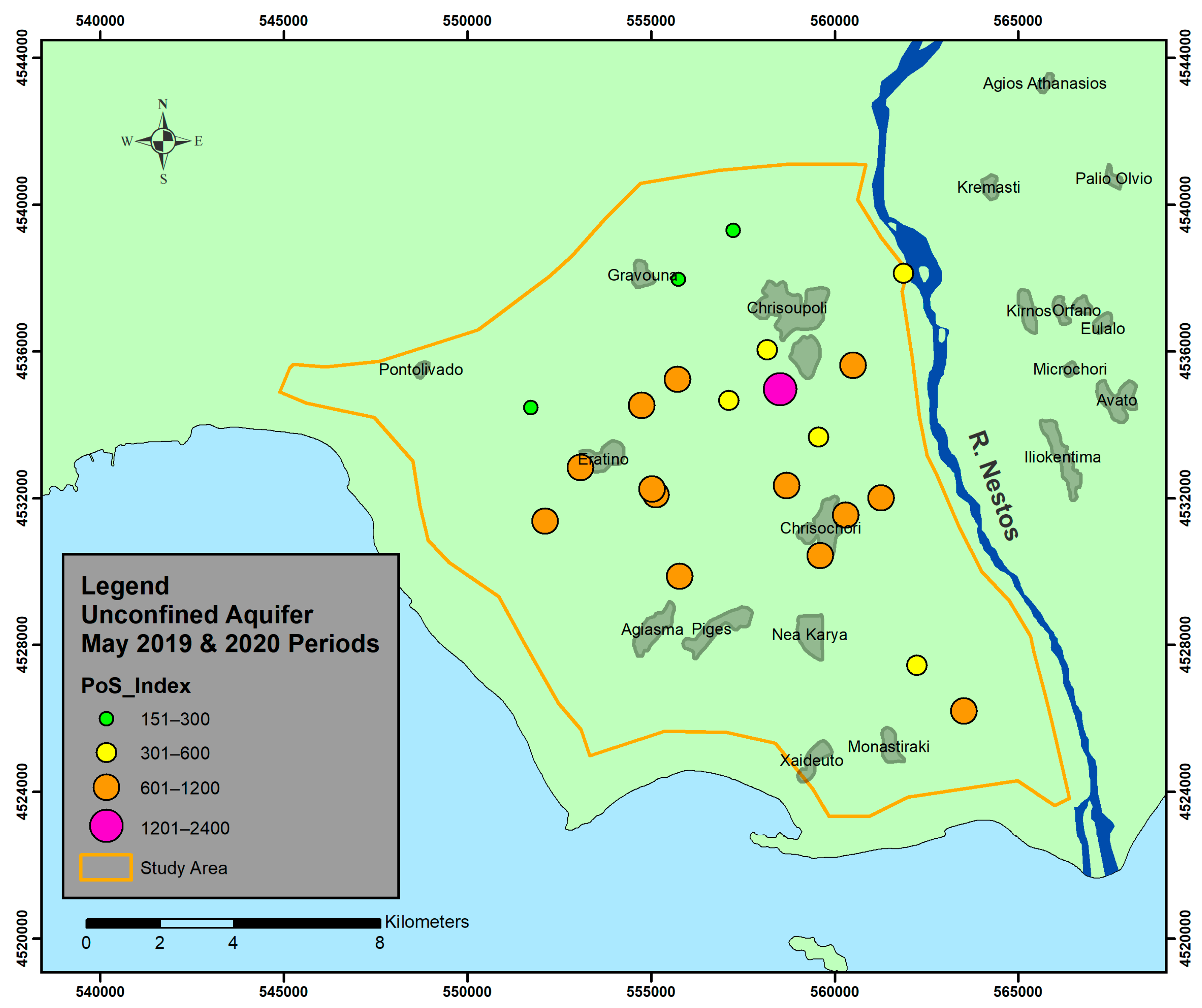
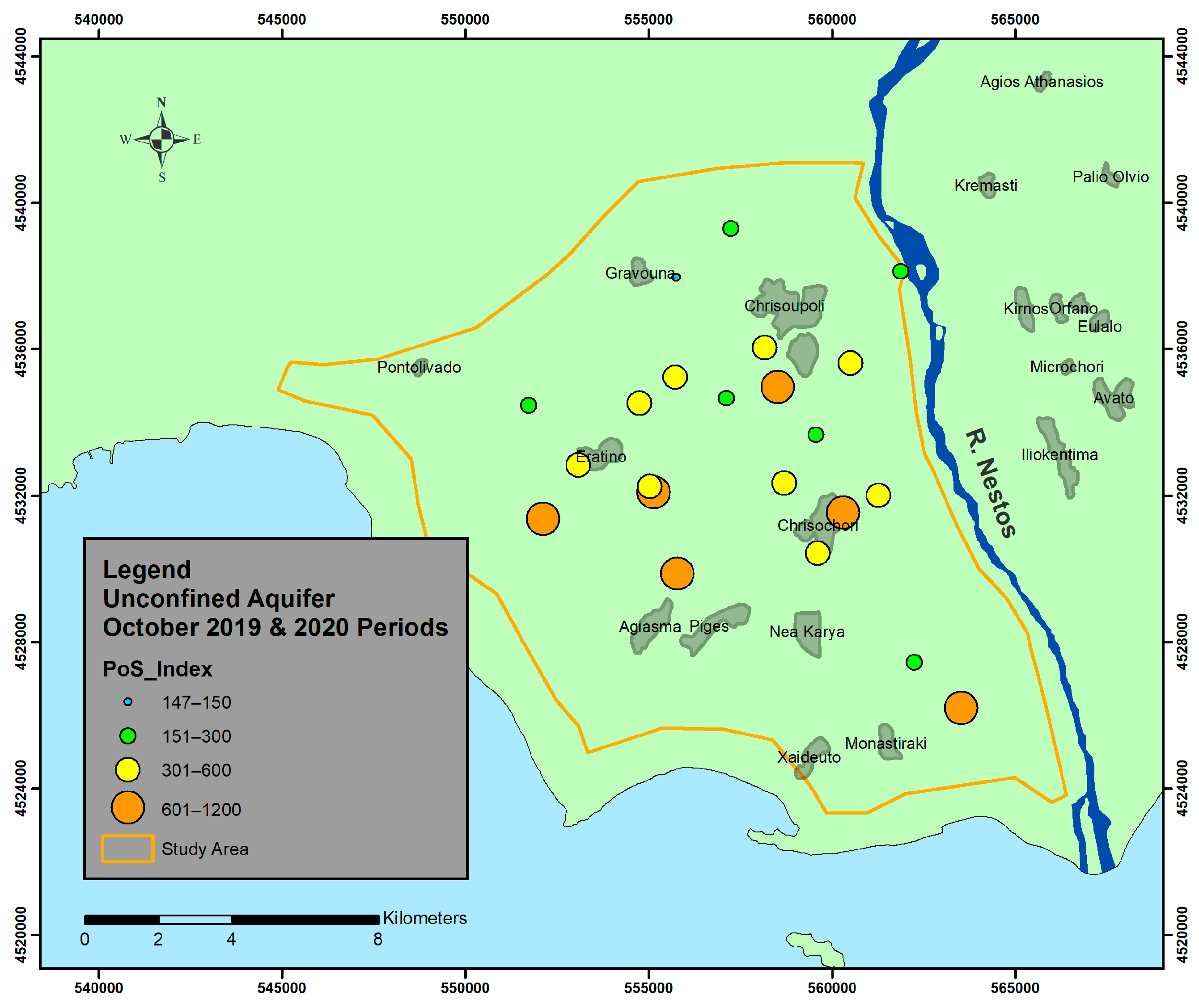
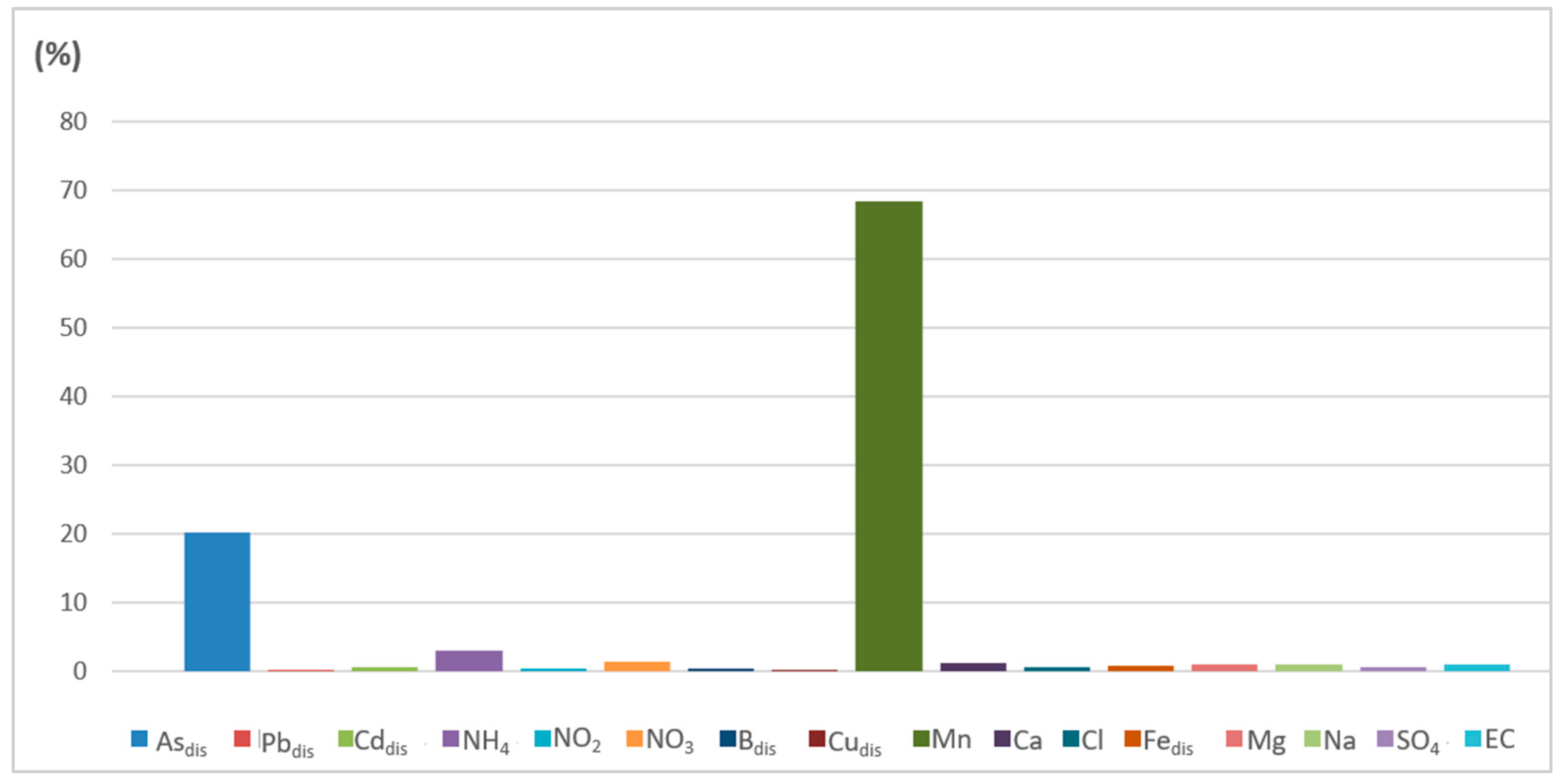
6. Results and Discussion

PoS index is calculated for the above 24 and 22 wells from the unconfined and the confined aquifers, respectively. In the following tables,

Table 7. Groundwater classification according to the PoS index (average May 2019 and 2020 values) (unconfined aquifer).

Well Code	PoS Index	Sample Classification		Quality Degradation Level
		Class	Color
25	546	3c/Mndis		Moderate
26	1152	4c/Asdis, Mndis		High
27	736	4a/Mndis		High
28	711	4a/Asdis, Mndis		High
29	541	3c/Mndis		Moderate
30	790	4a/Mndis		High
31	839	4b/Mndis		High
32	532	3c/Mndis		Moderate
33	236	2b/NH4+		Low
34	98	1/NO3-		None–Low
35	722	4a/Mndis		High
36	1002	4c/Mndis		High
37	420	3b/Mndis		Moderate
38	1005	4c/Mndis		High
39	186	2a/Asdis		Low
40	1054	4c/Mndis		High
41	454	3b/Asdis, NH4+, Mndis		Moderate
42	2305	5c/Asdis, Mndis		Very High
43	1019	4c/Asdis, Mndis		High
44	704	4a/Mndis		High
45	865	4b/Asdis, Mndis		High
46	946	4b/Mndis		High

,

Table 8. Groundwater classification according to the PoS index (average October 2019 and 2020 values) (unconfined aquifer).

Well Code	PoS Index	Sample Classification		Quality Degradation Level
		Class	Color
25	286	2c/Asdis, Mndis		Low
26	736	4a/Asdis, Mndis		High
27	577	3c/Asdis, Mndis		Moderate
28	519	3c/Asdis, Mndis		Moderate
29	278	2c/Asdis, Mndis		Low
30	638	4a/Mndis		High
31	522	3c/Mndis		Moderate
32	255	2c/Mndis		Low
33	288	2c/NH4+		Low
34	147	1/As, NO3-		None–Low
35	483	3b/Asdis, Mndis		Moderate
36	374	3a/Mndis		Moderate
37	297	2c/Asdis, Mndis		Low
38	721	4a/Asdis, Mndis		High
39	195	2a/Asdis		Low
40	785	4a/Asdis, Mndis		High
41	365	3a/Asdis, Mndis		Moderate
42	929	4b/Asdis, Mndis		High
43	501	3c/Asdis, Mndis		Moderate
44	691	4a/Mndis		High
45	407	3b/Asdis, Mndis		Moderate
46	594	3c/Mndis		Moderate

,

Table 9. Groundwater classification according to the PoS index (average May 2019 and 2020 values) (confined aquifer).

Sample Code	PoS Index	Sample Classification		Quality Degradation Level
		Class	Color
1	278	2c/Asdis		Low
2	2468	6/Asdis		Severe
3	526	3c/Mndis		Moderate
4	448	3b/Mndis		Moderate
5	816	4b/Asdis, Mndis		High
6	2242	5c/Asdis, Mndis		Very High
7	1156	4c/Asdis, Mndis		High
8	154	2a/Mndis		Low
9	1092	4c/Asdis, Mndis		High
10	440	3b/Asdis		Moderate
11	371	3a/Asdis		Moderate
12	134	1/Asdis		None–Low
13	852	4b/Asdis, Mndis		High
14	1243	5a/Asdis, Mndis		Very High
15	2443	6/Asdis		Severe
16	299	2a/Asdis		Low
17	380	3a/Asdis, Mndis		Moderate
18	824	4b/Asdis, Mndis		High
19	234	2b/Asdis, Mndis		Low
20	369	3a/Asdis		Moderate
21	387	3a/Asdis		Moderate
22	221	2b/NO3-		Low
23	351	3a/Asdis		Moderate
24	564	3c/Mndis		Moderate

and

Table 10. Groundwater classification according to the PoS index (average October 2019 and 2020 values) (confined aquifer).

Sample Code	PoS Index	Sample Classification		Quality Degradation Level
		Class	Color
1	218	2b/Asdis		Low
2	1657	5b/Asdis		Very high
3	457	3b/Asdis, Mndis		Moderate
4	258	2c/Mndis		Low
5	526	3c/Asdis, Mndis		Moderate
6	668	4a/Mndis		High
7	675	4a/Asdis, Mndis		High
8	90	1/Asdis, Mndis		None–low
9	929	4b/Asdis, Mndis		High
10	387	3a/Asdis		Moderate
11	326	3a/Asdis		Moderate
12	296	2c/Asdis		Low
13	343	3a/Asdis		Moderate
14	934	4b/Asdis, Mndis		High
15	1484	5a/Asdis		Very high
16	318	3a/Asdis		Moderate
17	168	2a/Asdis, Mndis		Low
18	508	3c/Asdis, Mndis		Moderate
19	165	2a/Asdis, Na+		Low
20	344	3a/Asdis		Moderate
21
22	247	2b/NO3-		Low
23	316	3a/Asdis		Moderate
24	458	3b/Mndis		Moderate

, the classification of the results are presented in accordance with the PoS index.

The following figures, Figure 3, Figure 4, Figure 5 and Figure 6, present the spatial distribution of the PoS Index for the unconfined and the confined aquifers.

Calculated PoS indices were used to study the spatiotemporal variations of the groundwater quality characteristics and depict the key parameters relating to the assessed conditions that could potentially cause adverse effects to humans and the natural environment. The following main observations can be made from the above tables (Table 7, Table 8, Table 9 and Table 10) and the spatial distribution depicted in Figure 3, Figure 4, Figure 5 and Figure 6.

• Unconfined aquifer

In the wet period of May, of the 22 total sampling points, 13 fall in the high-level degradation category, and only one sampling point (no. 42) falls into the very high-quality degradation category. In October, however, only 6 wells of the 22 belong in the high-level quality degradation category. Only samples of one well (no. 34) steadily present a low–none degradation level for both periods. In both periods, the main degradation factors are As and Mn. Water quality based on PoS appears higher during the wet period (May) compared to the dry (October) period (

Table 11. Comparative display of the two periods of the unconfined aquifer according to PoS index classes and identified dominant factors (Qfs).

	Wet Period (May 2019 and 2020)
PoS Index Class	1	2	3	4	5	6
No. of samples	1	2	5	13	1	0
% (percentage)	4.55	9.09	22.73	59.09	4.55	0.00
Dominant factors (Qfs)	NO3-	NH4+	Mndis	Mndis	Mndis
		Asdis	Asdis	Asdis	Asdis
			NH4+
	Dry Period (October 2019 and 2020)
PoS Index class	1	2	3	4	5	6
No. of samples	2	6	9	5	0	0
% (percentage)	9.09	27.27	40.91	22.73	0.00	0.00
Dominant factors (Qfs)	NO3-	Asdis	Asdis	Asdis
	Asdis	Mndis	Mndis	Mndis
		NH4+

).

• Confined aquifer

The overall picture presented is that the majority of the tested samples belong to the low and moderate degradation class for both periods (May and October). In the wet period (May), two samples (sampling points 2 and 15) demonstrate an exceptionally high level of degradation, two samples (sampling points 6 and 14) belong to very high degradation category, and two samples (sampling points 7 and 14) demonstrate a high degradation of quality. In the dry period of October, two samples (sampling points 2 and 15) belong to a high-degradation category, and three samples (sampling points 6, 7, and 14) belong to a high-degradation category. As in the unconfined aquifer, the main degradation factors are As and Mn, and a similar trend of improved overall quality status during the dry period of October is noted, although it is not pronounced (

Table 12. Comparative display of the two periods of the confined aquifer according to PoS index classes and identified dominant factors (Qf).

	Wet Period (May 2019 and 2020)
PoS Index Class	1	2	3	4	5	6
No. of samples	1	6	9	3	2	2
% (percentage)	4.17	25.00	37.50	12.50	8.33	8.33
Dominant factors (Qfs)	Asdis	Asdis	Asdis	Asdis	Asdis	Asdis
		Mndis	Mndis	Mndis	Mndis
		NH4+
		NO3-
	Dry Period (October 2019 and 2020)
PoS Index class	1	2	3	4	5	6
No. of samples	1	6	10	4	2	0
% (percentage)	4.35	26.09	43.48	17.39	8.70	0.00
Dominant factors (Qfs)	Asdis	Asdis	Asdis	Asdis	Asdis
	Mndis	Mndis	Mndis	Mndis
		Na+
		NO3-

).

As already stated, observing the distribution of the dominant factors (Qfs) among the six PoS index classes (Table 11 and Table 12), it is clear that As and Mn dominate (classes 2–6 for the two aquifers). Also, the other factors that affect the PoS index for classes 1 and 2 are NO₃, NH₄, and Na. Each substance, regardless of the P-class to which it belongs, may affect, either weakly or strongly, the overall groundwater quality status. Hence, PoS index is not biased towards toxic substances which may pose adverse effects to the environment (e.g., Pb, As, Hg) but also considers the major contribution of less toxic substances (e.g., Na, NO₃, NH₄, Mn) to the control of sample’s hydrogeochemistry and, consequently, to its overall environmental characteristics.

The cumulative contribution (%) of each of the parameters considered in the calculation of the PoS index for each of the periods (wet and dry) and the unconfined and confined aquifer is reported as derived from the following equation, Equation (4):

$$\mathrm{Contribution} (\%)=[\frac{\Sigma Qfi}{\Sigma Qfi+\Sigma Qfj+\dots +\Sigma Qfn}]\times 100$$

(4)

where ΣQfi is the total coefficient of the parameter i; ΣQfj is the total coefficient of the parameter j; and ΣQfn is the total coefficient of the parameter n.

The diagrams in Figure 7 and Figure 8 indicate that, for the unconfined aquifer, the main driving factor for groundwater quality degradation is Mn, at 68% for the wet period and approximately at 53% for the dry period. For the same aquifer, As is the second most important driving factor, at 20% and approximately 32% for the wet and dry seasons, respectively.

The diagrams in Figure 9 and Figure 10 indicate that, for the confined aquifer, the main driving factor for groundwater quality degradation is As, at about 56% for the wet and dry periods, respectively, followed by Mn, at about 32% and 28% for the wet and dry periods, respectively. The percentage of contribution for each of the other parameters for both aquifers and periods is less than 10%.

Analysis of the results (Table 11 and Table 12, Figure 7, Figure 8, Figure 9 and Figure 10) and their spatial distribution clearly suggest that the controlling factors of groundwater quality are As and Mn, which show a slight variability between the wet and the dry sampling periods and between the confined system and the unconfined aquifer. In both aquifers, the most degraded quality characteristics appear around the villages of Chrisochori and, secondarily, Chrisoupoli, which coincides well with the documented geothermal field of Nestos basin [38]. Hence, the elevated concentrations of these parameters may well be linked to the geological structure and the low enthalpy fields documented, as suggested in several cases of such fields across the world [39,40,41]. As already discussed, in applying the PoS methodology, a set of reference values needs to be considered, which, in our case, is the potability set of criteria, as practiced in many analogous applications. The origin of these parameters can clearly be traced back to natural geogenic processes. As such, the quality status of the assessed water samples may not be characterized as environmentally poor, but these samples indeed demonstrate impaired potability. Assuming the environmental quality characterization, the thresholds set in the implementation of the method for the particular parameters could have been shifted to higher values to account for the natural background concentrations due to the geothermal fields. Had this been the case, the implementation of the method would have not pinpointed these parameters at all. In fact, this is the rationale adopted by the EU in the framework of groundwater quality characterization, as the Water Framework Directive (2000/60/EEC) [42] focuses solely on the identification of human-induced elevated concentrations. However, this approach, which indeed seeks to assess deviations of groundwater quality from natural conditions, may fail to identify quality issues that are of essence in particular uses. As and Mn concentrations in the unconfined aquifer are indeed elevated but, in general, are lower than in the confined aquifer system, which could be argued to be the result of mixing of groundwater of the unconfined aquifer with surface water from the Nestos River that is mainly used for irrigation.

Even though nitrogen compounds are not the dominant controlling factors of groundwater quality in the assessed samples, they do contribute to its degradation. Especially in the unconfined aquifer, nitrogen compounds in the forms of NO₃^- and NO₄⁺ are apparent, and rather scattered, as reported in recent research works. Nitrogen concentrations are higher in the wet season compared to the dry season, and this may be attributed mainly to the following reasons: (a) during the wet season, the residues of fertilizers in the unsaturated zone are being leached down to the saturated zone due to the recharge the system receives, (b) parts of the unsaturated zone become saturated as the groundwater levels elevate in response to recharge, (c) typically, basic fertilization is practiced in late winter–early spring time, thus, in conjunction with the practiced over-irrigation, nitrogen leaches into the saturated zone. The confined aquifer system also exhibits nitrogen concentrations, but much lower, influencing the quality of the system to a much lower degree. The existence, however, of nitrogen compounds in the confined aquifer proves that the two systems are not entirely secluded by an aquiclude, which is a typical hydrogeological feature reported in other alluvial basins. Moreover, this finding may support the hypothesis of direct hydraulic interaction of the two aquifer systems through the production wells installed in the basin which tap all aquifer units drilled. Due to this phenomenon and the construction characteristics of the wells, it has been estimated that the preferential flow paths that develop through the gravel packs of the production wells may increase the vertical vector of the hydraulic conductivity of the confining geological strata by 2–3 orders of magnitude per basin—about the same scale as the study area.

Quality issues appear to be more concentrated in the confined aquifer system, especially around the Chrisochori–Chrisoupoli area, as already mentioned, that coincides with the geothermal field. On the contrary, the unconfined aquifer exhibits more scattered quality degradation issues that cover a much wider area, and these are, as already mentioned, related to nitrogen compounds. Clearly, nitrogen is an indicator of agricultural activity, the main economic activity in the region, as Nestos is amongst the high agricultural productivity basins of the country.

In contrast to conventional hydrochemical analyses concluded to date for the basin, salinization-related parameters do not seem to control or even strongly influence groundwater quality. Electric conductivity, or other conventionally considered parameters’ concentrations, such as Na⁺, for example, may often lead to misleading results or mask the quality-controlling factors, as these are clearly revealed in the studied case.

7. Conclusions

Accurate and reliable quality assessment is of essence in effective management of groundwater resources. As quick decisions need to be made, often by non-experts. understanding the key quality issues in a conclusive yet easy to conceive manner is necessary. To this end, index-based quality assessment methods offer a valuable tool. Amongst the numerous such methods proposed in the literature, PoS is a relatively new one that builds on the philosophy of quality assessments that are easy to use and comprehend, filtering out details that are essential and preserving accuracy.

Since, as its background, the method references toxicity studies listed in the literature and the quality standards for water intended for human consumption, it needs to be applied with great conscience and consideration with regards to the term “quality degradation level”. Hence, using unanimously accepted reference levels of a specific water use, the method yields a classification system that, however, does not necessarily imply degraded water quality “senso stricta”, but a potential harmful effect to biotic end users. It therefore follows that a critical view is always needed in carefully interpreting the results, thus avoiding misinterpretations. To this end, the term quality degradation level originally adopted by the method may be substituted with “quality category” or “level/class”, thus avoiding connotations that may be misleading. Indeed, the merit of the method compared to others, such as the chemical quality classification and assessment schemes for groundwater in the context of the 2000/60 EC Water Framework Directive [43]; 2006/118 EC Directives [44]; and 1st revision of the Thracian Water District (EL 12) [45], “Characterization and evaluation of the status of the groundwater bodies of the Thracian Water District (EL 12), Nestos Delta Groundwater System (EL 1200060)”, is that it employs a standardized approach regardless of the natural background levels for each constituent in each considered groundwater system, enabling a direct comparison of quality characteristics.

The results of the PoS index provide a new perspective to groundwater quality assessment. The key points of the deduced results are in line with the results of typical hydrochemical aproaches such as isoparametric spatial distribution maps, statistical analyses, and linear diagrams. PoS visualizes results in discrete classes and subclasses of quality degradation, thus offering a detailed assessment which does not lack spatial and temporal resolution. Highlighting the key parameters that control and shape the quality characteristics of the examined samples, the method helps focusing on the potential origin of the findings, these being either geogenic or manmade. In the studied case, it was deduced that the key quality issues relate to geothermal fields (As, Mn) and agricultural activities (nitrogen compounds), ruling out seawater intrusion as a key mechanism. Seawater intrusion could mistakenly have been assumed to be a key mechanism if not carefully interpreted through the study of conventional hydrochemical analysis methods. Based on this assessment, pressure analysis for a given catchment may easily confirm the potential origin of the quality degradation. As no actual restriction occurs to the parameters considered for the assessment, the method is adequately versatile to be used for comparisons between different aquifers of the same system, and of systems of different catchments, over various periods of time. Of course, any index-based assessment needs to be accompanied by in-depth analysis and study of the identified quality issues, employing conventional hydrochemical studies, statistical approaches, and hydrochemical diagrams, amongst others, to reach conclusive results and detailed, deep understanding of the dominant hydrogeochemical evolution mechanisms. Such analyses are indispensable, comprehended by experts, and constitute the full justification for groundwater quality assessment in support of the easy-to-comprehend PoS results.

References

1. Kim, J.; Kim, R.; Lee, J.; Chang, H. Hydrogeochemical characterization of major factors affecting the quality of shallow groundwater in the coastal area at Kimje in South Korea. Environ. Geol. 2003, 44, 189–478. [Google Scholar] [CrossRef]
2. Zhu, G.F.; Li, Z.Z.; Su, Y.H.; Ma, J.Z.; Zhang, Y.Y. Hydrogeochemical and isotope evidence of groundwater and recharge in Minqin Basin, Northwest China. J. Hydrol. 2007, 333, 239–251. [Google Scholar] [CrossRef]
3. Sandeep, K.G.; Tziritis, E.; Sudhir, K.S.; Jayant, K.T.; Abhay, K.S. Environmental monitoring of water resources with the use of PoS index: A case study from Subarnarekha River basin, India. Environ. Earth Sci. 2018, 77, 70. [Google Scholar] [CrossRef]
4. Piper, A.M. A graphic procedure in the geochemical interpretation of water analyses. Eos Trans. Am. Geophys. Union 1994, 25, 914–923. [Google Scholar]
5. Durov, S.A. Natural water and graphical representation of their composition. Dokl. Akad. Nauk USSR 1948, 59, 87–90. [Google Scholar]
6. Wilcox, L.V. Classification and Use of Irrigation Waters; Circular No. 969; U.S. Department of Agriculture: Washington, DC, USA, 1955; 19p. [Google Scholar]
7. Revelle, R. Criteria for recognition of sea water in ground waters. Trans. Am. Geophys. Union 1941, 22, 593–597. [Google Scholar]
8. Sivakumar, S.; Chandrasekaran, A.; Ravisankar, R.; Ravikumar, S.M.; Jebakumar, J.P.P.; Vijayagopal, P. Rements of natural radioactivity and evaluation of radiation hazards in coastal sediments of east coast of Tamilnadu, India using statistical approach. J. Taibah Univ. Sci. 2014, 8, 375–384. [Google Scholar] [CrossRef]
9. McKenna, J.E. An enhanced cluster analysis program with bootstrap significance testing for ecological community analysis. Environ. Model. Softw. 2003, 18, 205–220. [Google Scholar] [CrossRef]
10. Tziritis, E.; Panagopoulos, A.; Arampatzis, G. Development of an operational index of water quality (PoS) as a versatile tool to assist groundwater resources management and strategic planning. J. Hydrol. 2014, 517, 339–350. [Google Scholar] [CrossRef]
11. Tziritis, E.; Arampatzis, G.; Hatzigiannakis, E.; Panoras, G.; Panoras, A.; Panagopoulos, A. Quality characteristics and hydrogeochemistry of irrigation waters from three major olive groves in Greece. Desalination Water Treat. 2016, 57, 11582–11591. [Google Scholar] [CrossRef]
12. Tziritis, E.; Skordas, K.; Kelepertsis, A. The use of hydrochemical analyses and multivariate statistics for the characterization of groundwater resourses in the complex aquifer system. A case study in Amyros River basin, Thessaly, central Greece. Environ. Earth Sci. 2016, 75, 1–11. [Google Scholar] [CrossRef]
13. Salcedo-Sánchez, E.R.; Garrido Hoyos, S.E.; Esteller Alberich, M.V.; Martínez Morales, M. Application of water quality index to evaluate groundwater quality (temporal and spatial variation) of an intensively exploited aquifer (Puebla Valley, Mexico). Environ. Monit. Assess. 2016, 188, 1–20. [Google Scholar] [CrossRef]
14. Fernández, N.; Solano, F. Índices de Calidad y de Contaminación del Agua: Technical Report; Universidad de Pamplona: Norte de Santander, Colombia, 2005. (In Spanish) [Google Scholar]
15. Lumb, A.; Sharma, T.C.; Bibeault, J.-F.; Klawunn, P. A Comparative Study of USA and Canadian Water Quality Index Models. Water Qual. Expo. Health 2012, 3, 203–216. [Google Scholar] [CrossRef]
16. CCME. Canadian Environmental Quality Guidelines for the Protection of Aquatic Life; CCME water quality index: Technical report, 1.0; CCME: Winnipeg, MB, Canada, 2001. [Google Scholar]
17. Basha, U.I.; Rajasekhar, M.; Ghosh, S. Spatial assessment of groundwater quality using CCME-WQI and hydrochemical indices: A case study from Talupula Mandal, Ananthapuramu district, South India. Appl. Water Sci. 2022, 12, 168. [Google Scholar] [CrossRef]
18. Agency for Toxic Substances and Disease Registry (ATSDR). Detailed Data Table for the 2011 Priority List of Hazardous Substances. Agency for Toxic Substances and Disease Registry. 2011. Available online: https://stacks.cdc.gov/view/cdc/26622 (accessed on 20 November 2011).
19. Soltani, S.; Moghaddam, A.A.; Barzegar, R.; Kazemian, N.; Tziritis, E. Hydrogeochemistry and water quality of the Kordkandi-Duzduzan plain, NW Iran: Application of multivariate statistical analysis and PoS index. Environ. Monit. Assess. 2017, 189, 455. [Google Scholar] [CrossRef] [PubMed]
20. Vrouchakis, I. Hydrogeological Research Using Modern Management Tools in the Context of Qualitative and Quantitative Monitoring of the Aquifer System of the Tyrnavos Subbasin (Thessaly). Ph.D. Thesis, Athens Agronomist University, Athens, Greece, 2022. (In Greek). [Google Scholar]
21. Valko, M.M.H.C.M.; Morris, H.; Cronin, M.T.D. Metals, toxicity and oxidative stress. Curr. Med. Chem. 2005, 12, 1161–1208. [Google Scholar] [CrossRef] [PubMed]
22. International Toxicity Estimates for Risk (ITER). Toxicology Data Network. International Toxicity Estimates for Risk. 2011. Available online: https://pubmed.ncbi.nlm.nih.gov/15760833/ (accessed on 30 November 2012).
23. World Health Organization (WHO). Guidelines for Drinking-Water Quality, 4th ed.; WHO: Geneva, Switzerland, 2011.
24. Allen, M.J.; Yen, W.M. Introduction to Measurement Theory, printing ed.; Waveland Press: Long Grove, IL, USA, 2002. [Google Scholar]
25. Directive 2020/2184/EC; European Directive on the Quality of Water Intended for Human Consumption. Publication Office of the European Union: Luxembourg, 2020.
26. Delimani, P. Geological Changes of the Coastline in the Thrace Region and Impact on the Land Use of the Coastal Zone. Ph.D. Thesis, Department of Civil Engineering, Democritus University of Thrace, Xanthi, Greece, 2000. (In Greek). [Google Scholar]
27. American Public Health Association. APHA Standard Methods for The Examination of Water and Wastewater, 23rd ed.; American Public Health Association (APHA): Washington, DC, USA, 2017. [Google Scholar]
28. Novotny, V. Water Quality: Prevention, Identification and Management of Diffuse Pollution; Van Nostrand-Reinhold Publishers: New York, NY, USA, 1994; ISBN 0442005598. [Google Scholar]
29. DIN EN ISO 9963-1:1996-02; Wasserbeschaffenheit—Bestimmung der Alkalinität—Teil 1: Bestimmung der Gesamten und der Zusammengesetzten Alkalinität (ISO 9963-1:1994); Deutsche Fassung EN ISO 9963-1:1995. DIN Standards Committee Water Practice (NAW): Berlin, Germany, 1995; p. 24.
30. Keeney, D.R.; Nelson, D.W. Methods of Soil Analysis; Page, A.L., Ed.; Agronomy Monographs; American Society of Agronomy, Soil Science Society of America: Madison, WI, USA, 1983; ISBN 9780891189770. [Google Scholar]
31. Belcher, R.; Macdonald, A.M.G.; Parry, E. On mohr’s method for the determination of chlorides. Anal. Chim. Acta 1957, 16, 524–529. [Google Scholar] [CrossRef]
32. ISO 9964-3:1993; Water Quality—Determination of Sodium and Potassium—Part 3: Determination of Sodium and Potassium by Flame Emission Spectrometry. ISO: Geneva, Switzerland, 1993.
33. ISO 15586:2003; Water Quality—Determination of Trace Elements Using Atomic Absorption Spectrometry with Graphite Furnace [Online]. ISO: Geneva, Switzerland, 2003. Available online: https://www.iso.org/standard/38111.html (accessed on 13 May 2018).
34. Mohammed, E.; Mohammed, T.; Mohammed, A. Optimization of instrument conditions for the analysis for mercury, arsenic, antimony and selenium by atomic absorption spectroscopy. MethodsX 2018, 5, 824–833. [Google Scholar] [CrossRef]
35. Nehls, G.J.; Akland, G.G. Procedures for handling aerometric data. J. Air Pollut. Control Assoc. 1973, 23, 180–184. [Google Scholar] [CrossRef]
36. Clarke, J.U. Evaluation of censored data methods to allow statistical comparisons among very small samples with below detection limit observations. Environ. Sci. Technol. 1998, 32, 177–183. [Google Scholar] [CrossRef]
37. Hornung, R.W.; Reed, L.D. Estimation of average concentration in the presence of nondetectable values. Appl. Occup. Environ. Hyg. 1990, 5, 46–51. [Google Scholar] [CrossRef]
38. Kolios, N.; Koutsino, S.; Arvanitis, A.; Rydakis, G. Geothermal Situation in Northeastern Greece. In Proceedings of the World Geothermal Congress, Antalya, Turkey, 24–29 April 2005. [Google Scholar]
39. Davraz, A.; Nalbantçılar, M.T.; Varol, S.; Önden, İ. Hydrogeochemistry and reservoir characterization of the Konya geothermal elds, Central Anatolia/Turkey. Geochemistry 2022, 82, 125867. [Google Scholar] [CrossRef]
40. Morales-Simfors, N.; Bundschuh, J. Arsenic-rich geothermal fluids as environmentally hazardous materials—A global assessment. Sci. Total Environ. 2022, 817, 152669. [Google Scholar] [CrossRef] [PubMed]
41. Kaasalainen, H.; Stefánsson, A.; Giroud, N.; Arnórsson, S. The geochemistry of trace elements in geothermal fluids, Iceland. Appl. Geochem. 2015, 62, 207–223. [Google Scholar] [CrossRef]
42. Directive 2000/60/EC; European Framework Directive, Guidance Document 18: Guidance on Ground Water Status and Trend Assessment. European Commission: Luxembourg, 2009.
43. Directive 2000/60/EC; European Directive on the Establishing a Framework for Community Action in the Field of Water Policy. European Commission: Luxembourg, 2000.
44. Directive 2006/118/EC; European Directive on the Protection of Groundwater against Pollution and Deterioration. European Commission: Luxembourg, 2006.
45. 1st Review of the Thracian Water District (EL 12)—National Gazette of Greece No 4680B. 2017. Available online: https://wfdver.ypeka.gr/el/consultation-gr/1revision-consultation-gr/consultation-1revision-el12-gr/ (accessed on 13 May 2018).
Figure 1. Study area.
Water 16 00352 g001
Figure 2. Groundwater monitoring network points for the unconfined and the confined aquifers.
Water 16 00352 g002
Figure 3. Spatial distribution of PoS Index for the unconfined aquifer (average May 2019 and 2020 values).
Water 16 00352 g003
Figure 4. Spatial distribution of PoS Index for the unconfined aquifer (average October 2019 and 2020 values).
Water 16 00352 g004
Figure 5. Spatial distribution of PoS Index for the confined aquifer (average May 2019 and 2020 values).
Water 16 00352 g005
Figure 6. Spatial distribution of PoS Index for the confined aquifer (average October 2019 and 2020 values).
Water 16 00352 g006
Figure 7. Cumulative contribution of the presented parameters in applying the PoS index for all analyzed samples during the wet season (May 2019 and 2020) for the unconfined aquifer.
Water 16 00352 g007
Figure 8. Cumulative contribution of the presented parameters in applying the PoS index for all analyzed samples during the dry season (October 2019 and 2020) for the unconfined aquifer.
Water 16 00352 g008
Figure 9. Cumulative contribution of the presented parameters in applying the PoS index for all analyzed samples during the wet season (May 2019 and 2020) for the confined aquifer.
Water 16 00352 g009
Figure 10. Cumulative contribution of the presented parameters in applying the PoS index for all analyzed samples during the dry season (October 2019 and 2020) for the confined aquifer.
Water 16 00352 g010