Effect of the Likelihood Function on the Calibration of the Effective Manning Roughness Factor

Abstract

Hydrodynamic models (HMs) are tools for simulating flow behavior through the solution of conservation equations. These equations can have different degrees of simplification, which influence the model structure. One-dimensional (1D) HMs are still popular due to their simplicity. A crucial parameter for obtaining accurate 1D HM outputs is the effective Manning roughness factor (EMRF). The EMRF reflects additional numerical and dissipative aspects beyond boundary roughness. Although generalized likelihood uncertainty estimation (GLUE) is an important method for uncertainty analysis, it requires the selection of a likelihood function and a cutoff threshold. The goal of this study was to determine the effect of the likelihood function on the EMRF characteristics for mountain river morphologies, considering a certain cutoff threshold. The results show that the error model and the treatment of the residual in the objective function affect the EMRF range and limits in the studied reaches with a cascade or step pool. Furthermore, the analysis shows that these morphologies deviate from the model structure, which may affect the likelihood curve shape. Notably, the EMRF and measured roughness did not intersect in the studied reach with a plane bed, which is attributed to the presence of vegetation on the banks of that reach.

1. Introduction

Hydrodynamic models (HMs) are used to predict water motion through the solution of conservation equations [1,2]. HMs are used for predicting flood levels and flood risk [3]. One-dimensional (1D) HMs are still useful models due to their low data and computational resource requirements and ease of use [1,4,5]. Furthermore, the roughness factor is the main source of uncertainty in HMs when topographic data are accurately collected [3]. However, the roughness factor in a HM is an effective parameter, and its definition changes according to the flow description [6]. Thus, research on the behaviors of these parameters in 1D models is important. On the other hand, generalized likelihood uncertainty estimation (GLUE) is the most common methodology for reporting uncertainty [7] (other methods for determining uncertainty are described in Chowdhury and Egodawatta [8] and Yarahmadi et al. [9]). However, GLUE requires two arbitrary choices, likelihood functions and cutoff thresholds, which potentially alter the GLUE results [10]. This research addresses GLUE experiments on 1D HMs with different morphologies, different likelihood functions, different flow magnitudes, and a cutoff threshold based on water depth uncertainty. The goal of this study was to investigate the behavior of an effective roughness parameter, namely, the effective Manning roughness factor (EMRF), for different resistance phenomena and likelihood functions.

GLUE research has focused on likelihood curves, GLUE methodology modification, uncertainty bounds analysis, and comparisons with other uncertainty quantification methodologies. The likelihood curves are compared in two cases: (i) in a 1D unsteady flow HEC-RAS (U.S. Army Corps of Engineers) model of two reaches with discrete and continuous datasets [1] and (ii) in a two-dimensional (2D) shallow water equation (where convective and inertial terms are discarded), where two different types of likelihood functions are tested [11]. Some studies have focused on improving the GLUE framework. Aronica et al. [12] proposed a methodology to obtain the spatially distributed uncertainty within GLUE frameworks. The methodology was tested in two reaches using LISFLOOD: 1D modeling for the main channel and 2D modeling for the floodplain. Blasone et al. [13] proposed an adaptive sampling method for the prior parameter distribution. This methodology was tested in three different hydrological models. Papaioannou et al. [5] aimed to develop a generic methodology for roughness uncertainty assessment via 1D HMs. This approach includes a technique to determine the prior distribution of roughness and proposes an approach for the sampling procedure. The method was tested using a 1D HEC-RAS model. Some GLUE studies consider uncertainties in several parameters, which are individually and simultaneously propagated through the HMs. For example, this includes roughness and upstream flow in 1D models with uniform flow and steady shallow water equations [14] or flow–topography–roughness coupling in 1D HEC-RAS models [7]. Research has aimed to constrain the uncertainty bounds using different techniques: Bhola et al. [3] proposed a certain threshold for the objective function for HEC-RAS 2D, whereas Werner et al. [15] tested the utility of comprehensive calibration data to constrain the distributed flood plain roughness. The uncertainty quantification capabilities of GLUE have been assessed against various methodologies and model types. Reis et al. [16] compared GLUE with DREAM (Differential Evolution Adaptive Metropolis) in estimating discharge using the Manning equation. The calibrated parameters included Manning roughness and slope. Although both methods provided valid calibrated parameters for the model, DREAM exhibited a lower relative deviation between estimated and measured discharge, and its calibrated parameters showed a stronger correlation compared to those of GLUE. This et al. [17] compared GLUE with a Bayesian procedure for calibrating parameter values and assessing uncertainty in design flow estimates (quantiles) within catchment modeling. The Bayesian approach has demonstrated superiority in parameter identification and results in lower uncertainty in quantiles. In addition to GLUE, Mishra et al. [18] state that the turbulence model used in Computational Fluid Dynamics (CFDs) for aerospace systems is simple and cost-effective, yet capable of capturing specific characteristics of turbulence. Consequently, explicit uncertainty quantification in model predictions is essential. Mishra et al. [18] successfully tested a module in the CFD software SU2 that focused on estimating uncertainty and errors associated with turbulence closure models (EQUiPS).

The scope of this paper focuses on studying the EMRF under various dissipative processes and likelihood functions in mountain river reaches. To our knowledge, a similar study has not yet been presented. Section 2 describes different methodologies used to determine the EMRF and measured roughness (MR), considering the characteristics of the reaches studied, available data, GLUE testing, metrics, cutoff threshold, and HEC-RAS modeling. The results and discussion of the EMRF range and limits and a comparison of the obtained EMRFs and MRs are presented in Section 3 and Section 4. Finally, in Section 5, a summary of the sections and the main findings of this study are presented.

2. Materials and Methods

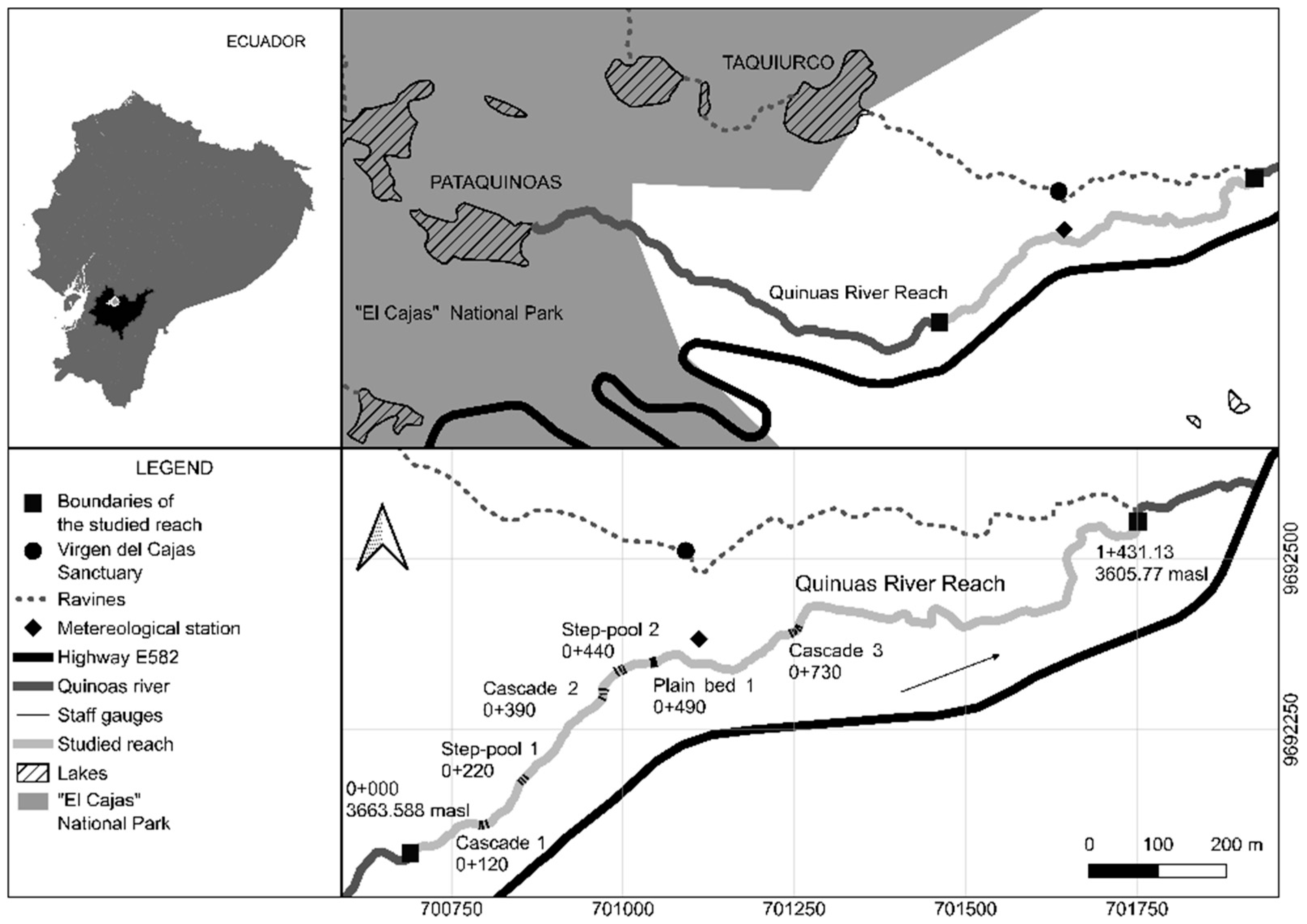
2.1. Studied Site

Figure 1 shows a map of part of the Quinuas River. This part of the river has been divided into six reaches based on morphology, where different field data have been collected. For the present study, three reaches were chosen as representatives of each morphology studied: Cascade 3, Plane bed 1, and Step pool 1. The names of the reaches and some geometric characteristics are shown in

Table 1. Geometric characteristics of the reaches studied.

Reach	Length (m)	Slope (%)	D84 (m)
Cascade 3	18.08	8.5	316.5 × 10−3
Step pool 1	12.22	6.1	251.2 × 10−3
Plane bed 1	6.26	3.16	218.8 × 10−3

.

2.2. Studied Available Data

Data on the reaches studied here are available and have already been used in some studies [19,20].

Table 2. Available data in the studied reaches.

Variable	Instrument	Methodology	Reference
Topography	Total station/Differential GPS	Point surveying of different cross-sections at the studied reaches	[20]
Water levels	Staff gauges	Measurement of water depth with a measuring tape in Staff gauges	[20]
Wetted width	Measuring tape	Measuring the water surface width excluding any protruding boulder width	[21]
Flow	HOBO U24-00 freshwater conductivity data loggers	Dilution gauging method	[22]
Velocity	Two HOBO U24-00 freshwater conductivity data loggers	U = L T-1, L is the distance between two instruments, T is the travel time estimated through the Harmonic method	[23]
Friction Slope	Staff gauges	Approximation through water surface slope using the measured staff gauges reads	[24]
Bed material size distribution	Sampling frame/Pebble-box	Pebble counting	[25]
Roughness parameter	Indirect determination	Darcy–Weisbach or Manning resistance equation	[26]

provides a summary of the different available data types for the reaches described in Table 1, which will hereafter be referred to as cascade, step pool, and plane bed.

2.3. GLUE Test

The GLUE methodology has been developed for calibration and uncertainty estimation [27]. In this article, GLUE has been utilized for calibration purposes. During modeling, various sources of error can arise, including model structures, boundary conditions, and observations. GLUE acknowledges that different combinations of these variables can produce acceptable simulations. GLUE consist of the following steps:

• Select the model parameter for calibration: the Manning roughness factor for the main channel.
• Choose a formal definition of likelihood. This function reflects how well the simulated results predict observations [27]. The functions used in this study are explained in the section titled “Likelihood Function”.
• Select the distribution of the parameter to be varied. In cases of limited knowledge, it is advisable to use a uniform distribution [1,27]. The roughness range for the cascade and plane bed is set at 0.03–0.5, whereas in the step pool, the range is expanded to 0.03–0.7, as the previous range was insufficient.
• Perform multiple simulations using the parameter sets within the chosen range. Each simulation is assigned a likelihood value. In this study, 20,000 runs were conducted for the three morphologies, with model outputs compared to water depth observations at three staff gauges (step pool and plane bed) and five staff gauges (cascade). An iterative process was implemented in the HEC-RAS controller using Visual Basic for Excel^® based on the code provided by Goodell [28]. Simulations with high likelihood values were retained. In this context, the separation between behavioral and non-behavioral models was achieved using a cutoff threshold (see Section CUTOFF Threshold).

2.4. Likelihood Function

Three likelihood functions were selected in this research, namely, the root mean square error (RMSE), the mean absolute error (MAE), and a modification of MAE called MAEU, which includes the uncertainty in water level measurements. The RMSE, MAE, and MAEU were modified to be dimensionless; this process is shown below.

2.4.1. First Likelihood Function: RMSEa

The RMSE is a metric commonly used during model performance evaluation [29]. According to Li et al. [10], this metric follows a square error model, where the residuals are squared. This metric has been used as a statistical measure when soft computing is used to predict Manning roughness parameters [9] or in the calibration of complex models encompassing urban hydrology, hydraulics, and stormwater quality [8].

$$\mathrm{RMSE}=\sqrt{{\displaystyle \frac{\sum _{\mathrm{i}=1}^n{\left({\mathrm{O}}_{\mathrm{i}} - {\mathrm{S}}_{\mathrm{i}}\right)}^2}{\mathrm{N}}}},$$

(1)

$$\mathrm{RMSEa}={\displaystyle \frac{\mathrm{RMSE}}{\overline{\mathrm{O}}}},$$

(2)

where O_i is the water depth observation [cm], S_i is the simulated water depth [cm], $\overline{\mathrm{O}}$ is the mean of the water depth observations [cm], and N is the number of data points.

2.4.2. Second Likelihood Function: MAEa

The MAE is a widely used metric to estimate model performance [29]. It follows an absolute error model, where the absolute value of the residuals is taken, as discussed by Li et al. [10]. The MAE was selected as the metric in Werner et al. [15] for discrete field data. Similarly, Li et al. [10] selected the MAE as a typical likelihood measure for hydrological model research, using the inverse MAE.

$$\mathrm{MAE}={\displaystyle \frac{1}{\mathrm{N}}}{\sum }_{\mathrm{i}=1}^{\mathrm{N}}\left|{\mathrm{O}}_{\mathrm{i}}-{\mathrm{S}}_{\mathrm{i}}\right|,$$

(3)

$$\mathrm{MAEa}={\displaystyle \frac{\mathrm{MAE}}{\overline{O}}},$$

(4)

2.4.3. Third Likelihood Function: MAEUa

MAEU is a modification of MAE in which the uncertainty in the measured water level (δa_h = 1.5%) is added. Thus, if a residual is less than the expected uncertainty, the residual will not be considered an error but rather an expected difference between the model outputs and observations.

$$\mathrm{if} \left\{\begin{array}{c}{\mathrm{Residual}}_{\mathrm{i}}<{\mathsf{\delta }\mathrm{a}}_{\mathrm{h}} {\mathrm{w}}_{\mathrm{i}}=0\\ {\mathrm{Residual}}_{\mathrm{i}}>{\mathsf{\delta }\mathrm{a}}_{\mathrm{h}} {\mathrm{w}}_{\mathrm{i}}=1\end{array}\right.,$$

(5)

$$\mathrm{MAEU}={\displaystyle \frac{{\sum }_{\mathrm{i}=1}^{\mathrm{n}}{\mathrm{residual}}_{\mathrm{i}} {\mathrm{w}}_{\mathrm{i}}}{\mathrm{N}}},$$

(6)

$$\mathrm{MAEUa}={\displaystyle \frac{\mathrm{MAEU}}{\overline{\mathrm{O}}}},$$

(7)

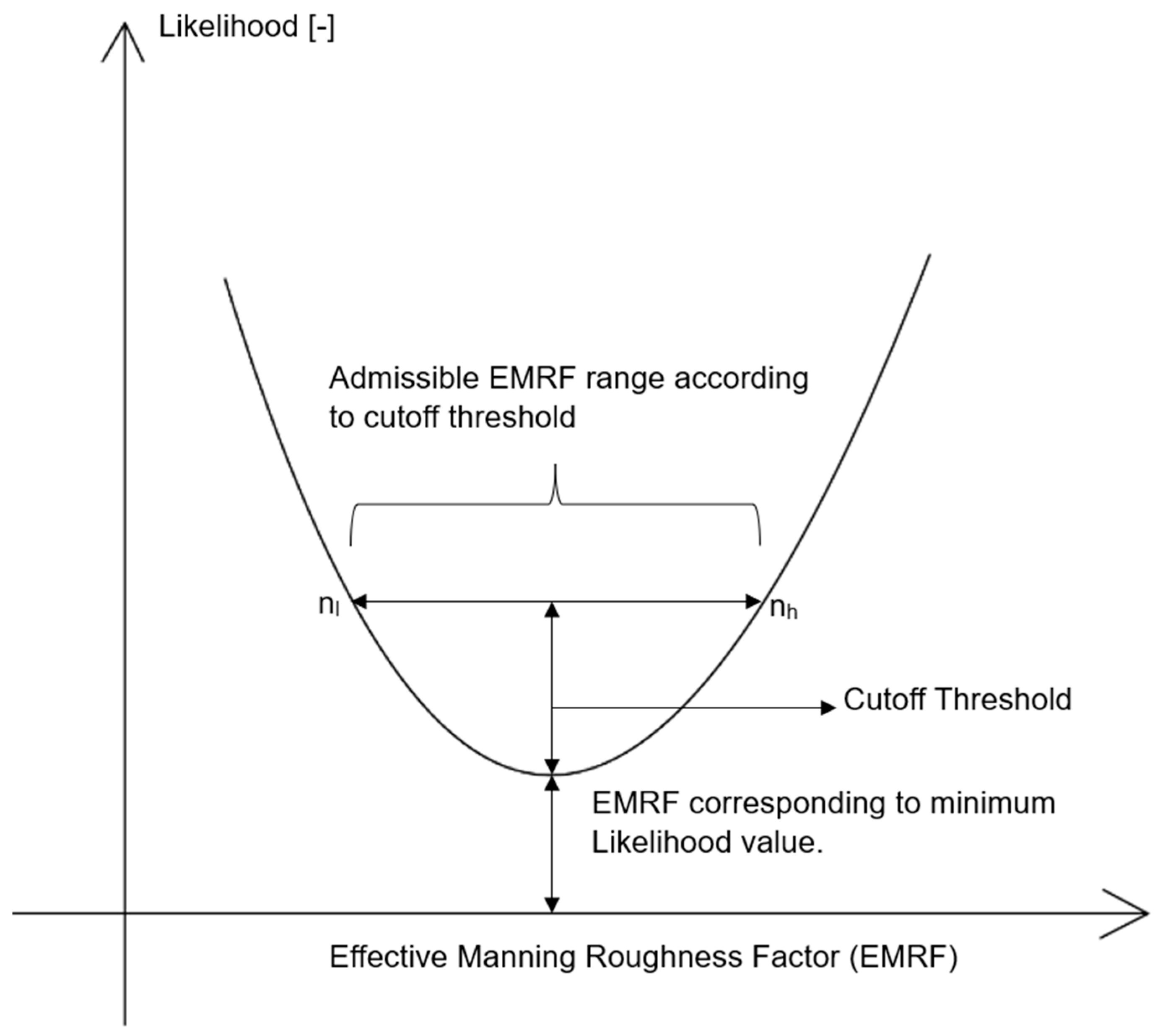
2.5. CUTOFF Threshold

Figure 2 depicts a scheme to illustrate the concept of the cutoff threshold, which obtains a model with acceptable performance [13]. Indeed, the cutoff threshold is an acceptable difference from the peak likelihood, which can be a certain value [13] or percentage [10,15]. However, in earlier work, the cutoff threshold was based on an arbitrary decision instead of an explicit criterion, as stated by Werner et al. [15]. In this research, the uncertainty in the water level measurements ($\mathsf{\delta }{\mathrm{a}}_{\mathrm{h}}$= 1.5%) was used as the cutoff threshold.

2.6. HEC-RAS

The selected reaches were run in the 1D component of HEC-RAS developed by the Hydrologic Engineering Center of the United States Army Corps of Engineers. All the HMs were run under steady-state conditions with a mixed flow regime. The HEC-RAS Controller^® allowed the iterative process to vary different parameters [28]. In this case, the main channel roughness parameter was chosen because the water level did not reach the floodplain. The reach topographic data were obtained from a combination of differential GPS and total station measurements to achieve high accuracy. The cross-sections were placed at crucial points, such as locations with changes in bed slope or abrupt alterations in XS shape. The boundary conditions were imposed upstream and downstream as normal depth. At some critical points, additional cross-sections were interpolated to stabilize the HM.

3. Results

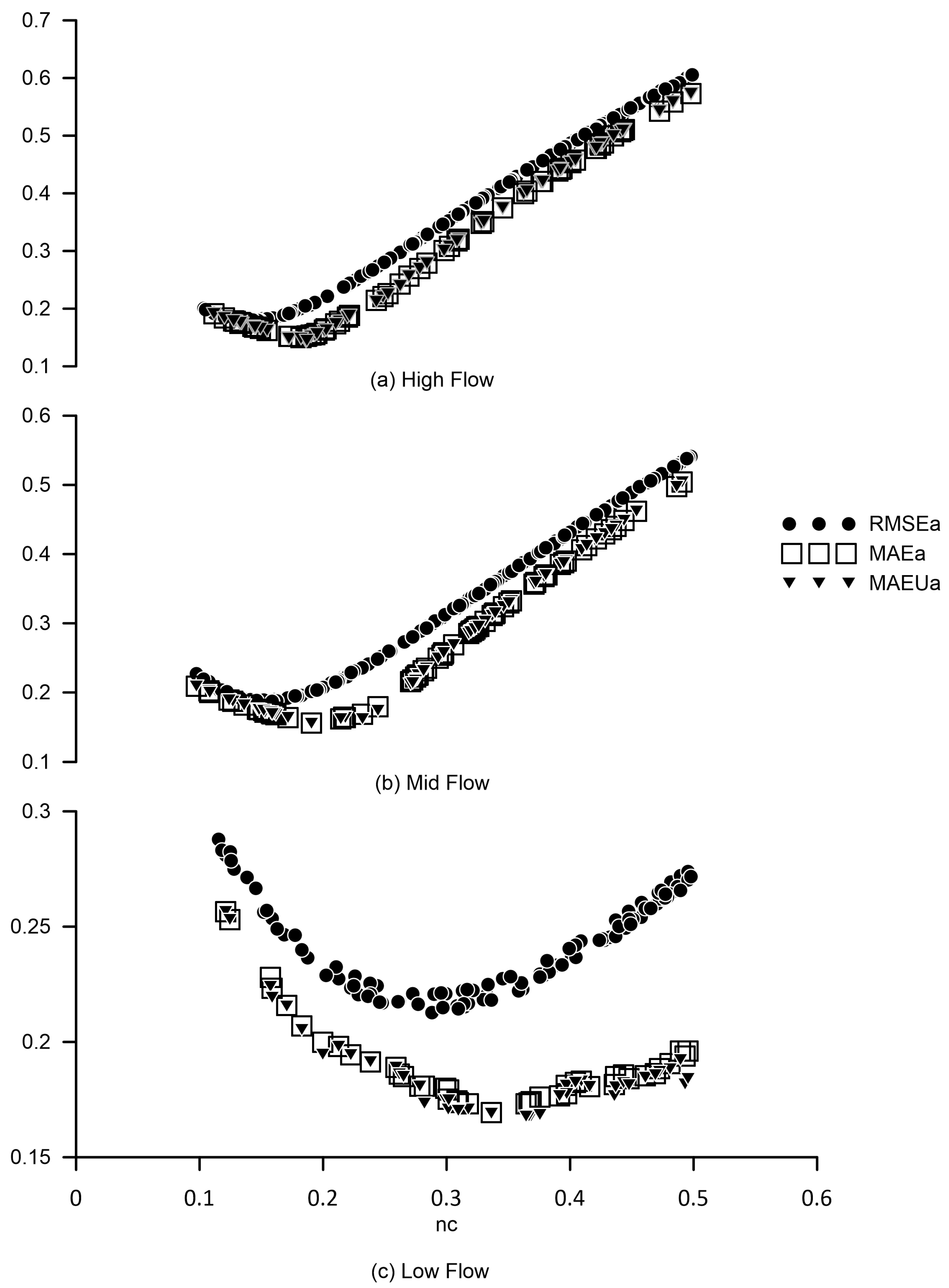
3.1. Effective Manning Rougheness Factor Range

The EMRF range, or nh-nl, in Figure 2 presents different magnitudes depending on the likelihood, morphology, and flow magnitude studied.

When the general trends of the EMRF in terms of MAEa, RMSEa, and MAEUa were analyzed, it was observed that the range of the EMRF decreased with increasing flow (refer to

Table 3. EMRF ranges (nh-nl in Figure 2).

Likelihood\Flow Magnitude	Cascade			Step Pool			Plane Bed
	Low	Moderate	High	Low	Moderate	High	Low	Moderate	High
L1: RMSEa	0.296	0.098	0.082	0.311	0.023	0.019	0.115	0.024	0.019
L2: MAEa	0.326	0.107	0.071	0.398	0.024	0.023	0.119	0.023	0.021
L3: MAEUa	0.323	0.110	0.063	0.373	0.023	0.021	0.090	0.023	0.019

). For low flow, the plane bed exhibited the lowest EMRF range (~0.1), in contrast to the cascade (~0.32) or the step pool (~0.36). Furthermore, in the moderate- and high-flow scenarios, the step pool and plane bed demonstrated comparable EMRF ranges (~0.02), whereas the cascade EMRF still varied between the moderate- (~0.1) and high-flow scenarios (0.07).

Differences can be observed in the EMRF ranges obtained from the MAEa, RMSEa, and MAEUa likelihoods (Table 3). Furthermore, the variations in EMRF ranges from these likelihood functions were small for the cascade and plane bed, indicating differences of less than 13% for only two extreme cases, with a difference of approximately 23%. In the step pool, the differences in EMRF ranges were more pronounced, particularly for the results of RMSEa and MAEa-MAEUa, with differences reaching 27%.

3.2. EMRF Limits

The influence of the likelihood function on EMRF limits (nl and nh according to Figure 2) was limited to the cascade morphology. MAEa and MAEUa produced similar nl/nh values for all the cases studied, with the maximum difference ranging from 0.21% to 11%, which was observed only in the extreme case of a plane bed and low flow. The average difference between MAEa and MAEUa was 3.03%. This difference is considered acceptable given that the uncertainty in the MR at this studied site was 22% [20]. Likewise, the nl/nh values obtained from the RMSEa and MAEa/MAEUa likelihoods exhibited similar differences between the step pool and plane bed morphologies. In the step pool, the maximum difference in nh between RMSEa and MAEa/MAEUa reached 13%, whereas the maximum difference in nl reached 1.65%, where the largest difference occurred for low flow. However, the remaining flows in this morphology produced differences in the nl/nh values of less than 3%. In the plane bed, the maximum difference in nl reached 11% at low flow, whereas in other scenarios, the difference in nl/nh was less than 1.5%. The cascade nl/nh values from RMSEa-MAEa/MAEUa demonstrate a stronger reliance on the likelihood function than those of the step pool or plane bed morphologies. Furthermore, nl, determined through RMSEa-MAEa/MAEUa, exhibited a maximum disparity of 41%, whereas nh displayed a maximum difference of 20%. Notably, these variations were absent during low flow, but were noticeable during moderate and high flows.

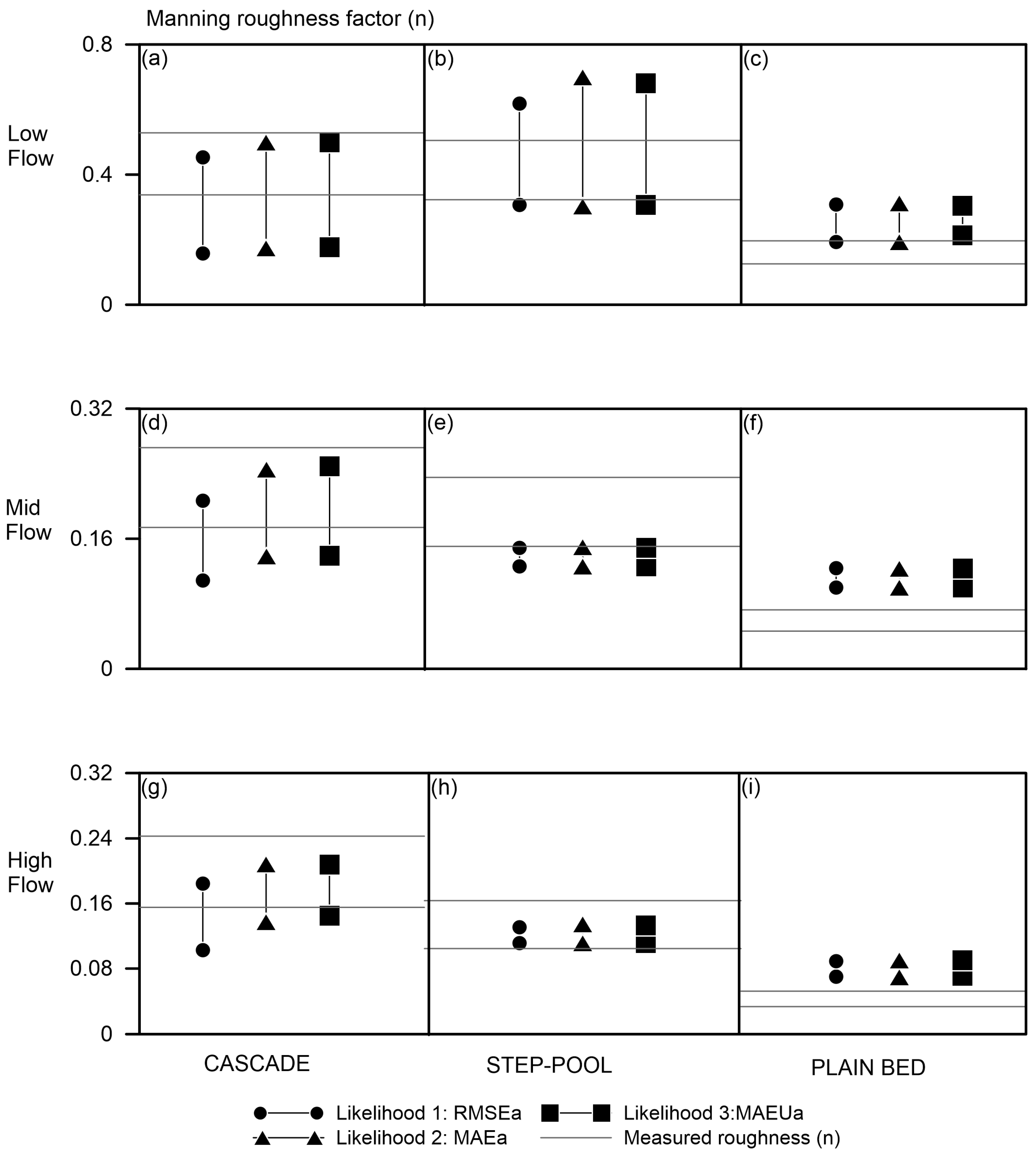
3.3. EMRF and Measured Roughness Factor

Figure 3 depicts the EMRF range and the measured Manning roughness (MR) values at the studied sites, considering uncertainty. The occurrence of the intersection between the EMRF and MR depends on morphology. In the cascade and step pool morphologies, all likelihoods resulted in EMRF intersecting with MR across all flow magnitudes, but in the plane bed, the intersection was limited to low flows.

4. Discussion

4.1. EMRF Range

The EMRF and topography are the major sources of uncertainty in HMs [1,12]. According to Bhola et al. [3], topography is usually seen as an input with the lowest uncertainty; however, there are studies in which this input has an important effect on model output. In this research, the topography was carefully measured with accurate instruments (see the description of the methodology in Section 2), so the main source of uncertainty was the EMRF. Moreover, the EMRF definition changes depending on the flow description (model structure [1]); thus, the EMRF encompasses different momentum and energy dissipation phenomena not included in the simplified conservation equations. In 1D HMs, roughness not only represents the interaction between water and the flow boundary but also the low-level representation of turbulence losses, three-dimensional (3D) effects, and incorrect geometry [3,6].

The general tendency of the EMRF range decreasing as flow increases is intuitive given that at low flow, there are more dissipative processes affecting water flow than at a moderate or high flow [30,31]. Furthermore, the cascade corresponds to higher EMRF ranges than those of the step pool or plane bed, given that the cascade likelihood curves (see Figure 4) are smoother than the step pool and plane bed likelihood curves (see Figure 5 and Figure 6). This behavior is attributed to the interaction of water with a random transverse and longitudinal distribution of boulders and cobbles in the cascade [32], where different flow patterns with different velocity components are present [24], even at high flows.

Different likelihoods have been used to test the effects of distinct error projections [29] on EMRF ranges. The cascade and plane bed EMRF ranges have shown no sensitivity to the residual weighting (RMSEa, MAEa [29]) or to the inclusion of uncertainty in the metrics (MAEUa [29]), but the step pool EMRF ranges are sensitive to residual weighting (RMSEa, MAEa) in the likelihood function. A possible explanation is the tumbling flow present in this morphology, where subcritical and supercritical flow occurs [30]. Moreover, the step pool likelihood curves do not have a ‘U’ shape. Instead, they start at an optimum, and the model performance decreases as the flow increases.

4.2. EMRF Limits

In the EMRF range, the EMRF limits show sensitivity to only the residual weighting in one morphology: the cascade morphology with moderate and high flows. Figure 4 shows that as the roughness parameter increases, the likelihood curves of the RMSEa and MAEa/MAEUa start to markedly differ. Moreover, the resulting optimum values are different. For example, in the cascade with low flow, the curves of RMSEa and MAEa/MAEUa have the same pattern, but the likelihood values are different.

4.3. EMRF and MR

During calibration, such as that performed here through GLUE, the goal is to find the parameters that provide results closer to observations while considering different uncertainties [11]. Uncertainty in the model results is related to the model structure (in this case, 1D) and uncertainties are related to the available information. The available information was meticulously quality controlled to reduce its associated uncertainty. Furthermore, the uncertainty in the MR was evaluated and estimated.

The EMRF is an important parameter in a HM, so an appropriate estimation of this parameter is a priority. However, frequently, data are insufficient, and the roughness parameter must be chosen using empirical equations, tables, or any other method developed to predict MR. Thus, if there is an intersection between EMRF and MR values, the methodologies developed to estimate MR can be used to estimate EMRF. These results indicate that the influence of the likelihood function on the intersection of the EMRF and MR depends on the magnitude of the flow resistance.

In this research, the cascade and step pool exhibited similar MR values, whereas the plane bed parameters were smaller [20]. Surprisingly, in the plane bed, the EMRF and MR intersected only at low flow. The reason for the lack of intersection in this morphology could be the presence of vegetation that enters the water, increasing the flow resistance [20]. Based on the current findings and insights from [20] Cedillo et al., when data are lacking, it is recommended to utilize nondimensional hydraulic geometry equations to estimate the EMRF while considering an uncertainty of 22%.

4.4. Comparison with the Literature Review

Pappenberger et al. [1] emphasize the need for a distinction between EMRF and MR, which are clearly not the same. The MR in this research was determined through field measurements described in the Methodology section (see Table 2). However, MR can be estimated based on data from the literature or the land use type [3]. The EMRF depends on the flow description, so this parameter can have different physical meanings [33]. This research aimed to compare the EMRF in the HEC-RAS steady-state model across different morphologies and MRs. Note that a similar study has not yet been presented in the literature. Most of the related literature addresses (i) changes in the likelihood curves due to the use of different calibration datasets [1] or different likelihood function types [11], (ii) improvements in GLUE to obtain spatially distributed uncertainty [12] or to improve the efficiency by modifying the sampling process of the prior parameter distribution [13], and (iii) comparisons of the predictability capacities of 1D and 2D inundation extents [33].

In this research, the EMRF range decreased as flow increased; however, another study indicates that low flows can complicate model predictions. In Reis et al. [16], which compares the uncertainty quantification of GLUE and DREAM when discharge was simulated using the Manning equation, the lowest simulated discharges consistently overestimated the observed values. In fact, that study identified a pattern similar to the one in this research, showing an inverse relationship between the relative deviation of estimated and measured discharges and flow magnitude. Furthermore, the discharge observations fell outside the uncertainty interval.

5. Conclusions

The effective Manning roughness factor (EMRF) has an important influence on hydrodynamic models (HMs) and is generally different from the measured roughness (MR). In this research, different analyses were developed to understand EMRF behavior in one-dimensional (1D) stationary models (SMs). Thus, the generalized likelihood uncertainty estimation (GLUE) methodology was implemented in a 1D SM with different likelihood functions and a threshold equal to the water depth measurement uncertainty. Three mountain river reaches were simulated with different morphologies (distinct flow patterns and dissipative processes). These studied reaches have detailed geometries, bed material composition, flow, MR, and field measurement uncertainty data available. The goal of this research was to analyze the influence of morphology and the likelihood function on the EMRF ranges, EMRF limits, and differences between the EMRF and MR.

Different results were obtained from different tests, where the influence of the morphology and flow magnitude on the EMRF vary. The tendency for the EMRF range to decrease as flow increases is attributed to the occurrence of different flow dissipative processes in mountain rivers. The influence of these processes decreases as flow increases. Moreover, the cascade and step pool morphologies were sensitive to likelihood residual weighting, affecting the EMRF range and EMRF limits. A common characteristic of these morphologies is the flow characteristics and resistance phenomena affecting the shapes of the likelihood curves. For example, the likelihood curves of the step pool start at an optimum, and as the roughness parameter increases, model performance decreases. The cascade likelihood curves differ at a certain roughness value. Moreover, the comparison of the EMRF and MR revealed that in the cascade and step pool, there was an intersection of these parameters. However, in the plane bed, there was an intersection of these parameters only at low flows. This difference may be due to the presence of vegetation on the banks.

References

1. Pappenberger, F.; Beven, K.; Horritt, M.; Blazkova, S. Uncertainty in the Calibration of Effective Roughness Parameters in HEC-RAS Using Inundation and Downstream Level Observations. J. Hydrol. 2005, 302, 46–69. [Google Scholar] [CrossRef]
2. Teng, J.; Jakeman, A.J.; Vaze, J.; Croke, B.F.W.; Dutta, D.; Kim, S. Flood Inundation Modelling: A Review of Methods, Recent Advances and Uncertainty Analysis. Environ. Model. Softw. 2017, 90, 201–216. [Google Scholar] [CrossRef]
3. Bhola, P.K.; Leandro, J.; Disse, M. Reducing Uncertainty Bounds of Two-Dimensional Hydrodynamic Model Output by Constraining Model Roughness. Nat. Hazards Earth Syst. Sci. 2019, 19, 1445–1457. [Google Scholar] [CrossRef]
4. Cook, A.; Merwade, V. Effect of Topographic Data, Geometric Configuration and Modeling Approach on Flood Inundation Mapping. J. Hydrol. 2009, 377, 131–142. [Google Scholar] [CrossRef]
5. Papaioannou, G.; Vasiliades, L.; Loukas, A.; Aronica, G.T. Probabilistic Flood Inundation Mapping at Ungauged Streams Due to Roughness Coefficient Uncertainty in Hydraulic Modelling. Adv. Geosci. 2017, 44, 23–34. [Google Scholar] [CrossRef]
6. Morvan, H.; Knight, D.; Wright, N.; Tang, X.; Crossley, A. The Concept of Roughness in Fluvial Hydraulics and Its Formulation in 1D, 2D and 3D Numerical Simulation Models. J. Hydraul. Res. 2008, 46, 191–208. [Google Scholar] [CrossRef]
7. Jung, Y.; Merwade, V. Uncertainty Quantification in Flood Inundation Mapping Using Generalized Likelihood Uncertainty Estimate and Sensitivity Analysis. J. Hydrol. Eng. 2012, 17, 507–520. [Google Scholar] [CrossRef]
8. Chowdhury, A.; Egodawatta, P. Automatic Model Calibration of Combined Hydrologic, Hydraulic and Stormwater Quality Models Using Approximate Bayesian Computation. Water Sci. Technol. 2022, 86, 321–332. [Google Scholar] [CrossRef]
9. Yarahmadi, M.B.; Parsaie, A.; Shafai-Bejestan, M.; Heydari, M.; Badzanchin, M. Estimation of Manning Roughness Coefficient in Alluvial Rivers with Bed Forms Using Soft Computing Models. Water Resour. Manag. 2023, 37, 3563–3584. [Google Scholar] [CrossRef]
10. Li, Z.; Yang, T.; Zhang, N.; Zhang, Y.; Wang, J.; Xu, C.-Y.; Shi, P.; Qin, Y. Understanding the Impacts Induced by Cut-off Thresholds and Likelihood Measures on Confidence Interval When Applying GLUE Approach. Stoch. Environ. Res. Risk Assess. 2022, 36, 1215–1241. [Google Scholar] [CrossRef]
11. Aronica, G.; Hankin, B.; Beven, K. Uncertainty and Equifinality in Calibrating Distributed Roughness Coefficients in a Flood Propagation Model with Limited Data. Adv. Water Resour. 1998, 22, 349–365. [Google Scholar] [CrossRef]
12. Aronica, G.; Bates, P.D.; Horritt, M.S. Assessing the Uncertainty in Distributed Model Predictions Using Observed Binary Pattern Information within GLUE. Hydrol. Process. 2002, 16, 2001–2016. [Google Scholar] [CrossRef]
13. Blasone, R.S.; Vrugt, J.A.; Madsen, H.; Rosbjerg, D.; Robinson, B.A.; Zyvoloski, G.A. Generalized Likelihood Uncertainty Estimation (GLUE) Using Adaptive Markov Chain Monte Carlo Sampling. Adv. Water Resour. 2008, 31, 630–648. [Google Scholar] [CrossRef]
14. Bozzi, S.; Passoni, G.; Bernardara, P.; Goutal, N.; Arnaud, A. Roughness and Discharge Uncertainty in 1D Water Level Calculations. Environ. Model. Assess. 2015, 20, 343–353. [Google Scholar] [CrossRef]
15. Werner, M.G.F.; Hunter, N.M.; Bates, P.D. Identifiability of Distributed Floodplain Roughness Values in Flood Extent Estimation. J. Hydrol. 2005, 314, 139–157. [Google Scholar] [CrossRef]
16. Reis, G. da C. dos; Pereira, T.S.R.; Faria, G.S.; Formiga, K.T.M. Analysis of the Uncertainty in Estimates of Manning’s Roughness Coefficient and Bed Slope Using GLUE and DREAM. Water 2020, 12, 3270. [Google Scholar] [CrossRef]
17. Cu Thi, P.; Ball, J.E.; Dao, N.H. Uncertainty Estimation Using the Glue and Bayesian Approaches in Flood Estimation: A Case Study—Ba River, Vietnam. Water 2018, 10, 1641. [Google Scholar] [CrossRef]
18. Mishra, A.A.; Mukhopadhaya, J.; Iaccarino, G.; Alonso, J. Uncertainty Estimation Module for Turbulence Model Predictions in SU2. AIAA J. 2019, 57, 1066–1077. [Google Scholar] [CrossRef]
19. Cedillo, S.; Sánchez-Cordero, E.; Timbe, L.; Samaniego, E.; Alvarado, A. Resistance Analysis of Morphologies in Headwater Mountain Streams. Water 2021, 13, 2207. [Google Scholar] [CrossRef]
20. Cedillo, S.; Sánchez-Cordero, E.; Timbe, L.; Samaniego, E.; Alvarado, A. Patterns of Difference between Physical and 1-D Calibrated Effective Roughness Parameters in Mountain Rivers. Water 2021, 13, 3202. [Google Scholar] [CrossRef]
21. Lee, A.J.; Ferguson, R.I. Velocity and Flow Resistance in Step-Pool Streams. Geomorphology 2002, 46, 59–71. [Google Scholar] [CrossRef]
22. Hudson, R.; Fraser, J. Introduction to Salt Dilution Gauging for Streamflow Measurement, Part IV: The Mass Balance (or Dry Injection) Method. Streamline Watershed Manag. Bull. 2005, 9, 6–12. [Google Scholar]
23. Nitsche, M.; Rickenmann, D.; Kirchner, J.W.; Turowski, J.M.; Badoux, A. Macroroughness and Variations in Reach-Averaged Flow Resistance in Steep Mountain Streams. Water Resour. Res. 2012, 48, W12518. [Google Scholar] [CrossRef]
24. David, G.C.L.; Wohl, E.; Yochum, S.E.; Bledsoe, B.P. Controls on Spatial Variations in Flow Resistance along Steep Mountain Streams. Water Resour. Res. 2010, 46, W03513. [Google Scholar] [CrossRef]
25. Bunte, K.; Abt, S.R. Sampling Surface and Subsurface Particle-Size Distributions in Wadable Gravel- and Cobble-Bed Streams for Analyses in Sediment Transport, Hydraulics, and Streambed Monitoring; US Department of Agriculture, Forest Service, Rocky Mountain Research Station: Fort Collins, CO, USA, 2001; ISBN RMRS-GTR-74. [Google Scholar]
26. Comiti, F.; Cadol, D.; Wohl, E. Flow Regimes, Bed Morphology, and Flow Resistance in Self-Formed Step-Pool Channels. Water Resour. Res. 2009, 45, W04424. [Google Scholar] [CrossRef]
27. Beven, K.; Binley, A. The Future of Distributed Models: Model Calibration and Uncertainty Prediction. Hydrol. Process. 1992, 6, 279–298. [Google Scholar] [CrossRef]
28. Goodell, C. Breaking the HEC-RAS Code: A User’s Guide to Automating HEC-RAS; h2ls: Portland, OR, USA, 2014. [Google Scholar]
29. Chai, T.; Draxler, R.R. Root Mean Square Error (RMSE) or Mean Absolute Error (MAE)?—Arguments against Avoiding RMSE in the Literature. Geosci. Model Dev. 2014, 7, 1247–1250. [Google Scholar] [CrossRef]
30. Curran, J.H.; Wohl, E.E. Large Woody Debris and Flow Resistance in Step-Pool Channels, Cascade Range, Washington. Geomorphology 2003, 51, 141–157. [Google Scholar] [CrossRef]
31. Wohl, E. Mountain Rivers; American Geophysical Union: Washington, DC, USA, 2000; Volume 14, ISBN 0-87590-318-5. [Google Scholar]
32. Montgomery, D.R.; Buffington, J.M. Channel-Reach Morphology in Mountain Drainage Basins. Geol. Soc. Am. Bull. 1997, 109, 596–611. [Google Scholar] [CrossRef]
33. Horritt, M.S.; Bates, P.D. Evaluation of 1D and 2D Numerical Models for Predicting River Flood Inundation. J. Hydrol. 2002, 268, 87–99. [Google Scholar] [CrossRef]
Figure 1. Map of the reaches studied: Cascade 3, Step pool 1, and Plane bed 1.
Water 16 02879 g001
Figure 2. Explanation of the cutoff threshold.
Water 16 02879 g002
Figure 3. Effect of likelihood on the admissible EMRF and Measured roughness in comparison with EMRF. Cascade: (a) Low flow, (d) Mid flow, (g) High flow. Step-pool: (b) Low flow, (e) Mid flow, (h) High flow. Plain bed: (c) Low flow, (f) Mid flow, (i) High flow.
Water 16 02879 g003
Figure 4. Different likelihood functions for Cascade 3.
Water 16 02879 g004
Figure 5. Different likelihood functions for Step pool 1.
Water 16 02879 g005
Figure 6. Different likelihood functions for Plane bed 1.
Water 16 02879 g006