Abstract
Recent studies have shown the potential of transformer-based neural networks in increasing prediction capacity. However, classical transformers present several problems such as computational time complexity and high memory requirements, which make Long Sequence Time-Series Forecasting (LSTF) challenging. The contribution to the prediction of time series of flood events using deep learning techniques is examined, with a particular focus on evaluating the performance of the Informer model (a particular implementation of transformer architecture), which attempts to address the previous issues. The predictive capabilities of the Informer model are explored and compared to statistical methods, stochastic models and traditional deep neural networks. The accuracy, efficiency as well as the limits of the approaches are demonstrated via numerical benchmarks relating to real river streamflow applications. Using daily flow data from the River Test in England as the main case study, we conduct a rigorous evaluation of the Informer efficacy in capturing the complex temporal dependencies inherent in streamflow time series. The analysis is extended to encompass diverse time series datasets from various locations (>100) in the United Kingdom, providing insights into the generalizability of the Informer. The results highlight the superiority of the Informer model over established forecasting methods, especially regarding the LSTF problem. For a forecast horizon of 168 days, the Informer model achieves an NSE of 0.8 and maintains a MAPE below 10%, while the second-best model (LSTM) only achieves −0.63 and 25%, respectively. Furthermore, it is observed that the dependence structure of time series, as expressed by the climacogram, affects the performance of the Informer network.
1. Introduction
Flood events refer to the natural phenomena characterized by the overflow or inundation of land areas that are typically dry, caused by excessive accumulation of water. These events can occur due to various factors such as heavy rainfall, snowmelt, dam failure, or coastal surges. Floods are of huge importance worldwide as natural disasters that affect different regions, leaving a profound impact on societies [1]. They transcend geographical boundaries and affect millions of lives around the world, making them a critical area of study and research. Understanding the impacts and mitigating the risks associated with flood events is of paramount importance to safeguard human life and minimise socio-economic and environmental damage. They can result in loss of life, property damage, displacement of communities, disruption of essential services, and long-term ecological consequences. The severity and frequency of flooding events vary globally, making accurate forecasting and alertness crucial for effective disaster management and mitigation strategies. In the context of the above, the accurate prediction of daily river streamflow, which constitutes an important factor in flooding, is essential.
Precise streamflow forecasting is particularly needed in agricultural water management, because it affects irrigation scheduling, mitigation of drought and flood, and many other actions that ensure agriculture stability and optimize crop yields. On the other hand, timely and accurate forecasts can reduce the impact of drought, allowing for proactive water management strategies through adjustments in irrigation and water-saving plans ahead of the dry seasons [2]. Likewise, streamflow predictions are vital in flood prevention and management, thus protecting farmland from flooding and associated losses. Hence, this pre-emptive approach provides a robust tool for agriculture water managers to make informed decisions for improving the overall efficiency of water use in agriculture.
Various techniques are employed to achieve accurate and reliable results for estimating river streamflow, most of which are either physically based models or data-driven. Physically based models for streamflow prediction depend on specific hydrological hypotheses and necessitate extensive hydrological data for effective calibration [3]. They represent hydrological systems truthfully and show what is happening with the processes involved. They also prove particularly beneficial when a deep understanding of the physical processes is essential, such as assessing the impact of land use changes or climatic variations on streamflow [4]. Beyond data constraints [5], these models often require complex parameterization, a process prone to challenges and imprecision. Unfortunately, the calibration of these models is resource-intensive and time-consuming. As a result, there is a growing interest in enhancing data-driven models for streamflow prediction, which are more efficient and cost-effective.
For time series prediction of river streamflow, advanced approaches like statistical models, such as autoregressive integrated moving average (ARIMA) [6], and seasonal decomposition methods are widely used. These statistical models leverage historical data to forecast future flow values, considering seasonality and trends. Moreover, machine learning algorithms—including k-Nearest Neighbors (KNN) [7], Artificial Neural Networks (ANN), Light Gradient Boosting Machine Regressor (LGBM), Linear Regression (LR), Multilayer Perceptron (MLP), Random Forest (RF), Stochastic Gradient Descent (SGD), Extreme Gradient Boosting Regression (XGBoost), and Support Vector Regression (SVR)—have been widely used as well [4]. There is also great interest in deep learning methods, like Recurrent Neural Networks (RNN), Long Short-Term Memory (LSTM) [8] networks and Convolutional Neural Networks (CNN) [9]. Some other models follow a combined methodology utilizing artificial neural networks that obey any given law of physics, known as Physics Informed Neural Networks (PINNs) [10].
In recent years, modern deep learning models like Transformers, have gained popularity (Figure 1) for many tasks, including time series prediction, due to their ability to capture complex temporal long-range dependencies and non-linear patterns. Through an attention mechanism, transformers grant a complete and interrelated view of the entire time series being analyzed. These methods could play a crucial part in accurate forecasting of river streamflow and thus empowering water resource managers to make informed decisions for flood management, drought mitigation, and sustainable water allocation.
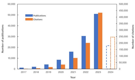
Figure 1.
The number of publications and citations per year from 2017 (until 2 June 2024), related to Transformer networks (data were obtained from Dimensions AI [11], using the keywords: “transformer model”, “attention mechanism”, “self-attention in neural networks”).
1.1. Literature Review
1.1.1. Traditional Methods
Time series forecasting has attracted great scientific interest among researchers of many disciplines and for the analysis of various tasks, including the area of hydrology and streamflow prediction. Many algorithms have been used over the years to solve the problem of forecasting, from classical statistical methods to advanced deep learning algorithms. In the book of Box et al. [12], there are several statistical methods and techniques used to analyse and forecast time series data, including the Autoregressive Integrated Moving Average (ARIMA) model [13]. This model follows the Markov process and creates an autoregressive model for recursive sequential forecasting. Exponential Smoothing [14] is used to examine the practical application for handling trend, seasonality, and other components of time series data. Similar models have been applied for streamflow forecasting problem for the last 50 years, like Moving Average (MA), Auto Regressive Moving Average (ARMA), Linear Regression (LR), and Multiple Linear Regression (MLR) [15,16,17].
Some limitations of these traditional techniques include the frequent assumption that the time series data are linear and stationary. Models such as ARIMA and exponential smoothing have limited ability to approximate complex patterns of time series data, such as anomalies, abrupt changes, slope changes, and non-linear relationships. Another challenge of traditional models is the limitations they may have when processing large-scale time series data or high-dimensional data [18]. As a result, researchers have focused on crafting models designed to mitigate the limitations inherent in conventional models, e.g., data-driven approaches in the broader domain of Artificial Intelligence (AI).
1.1.2. Machine Learning Approaches
In the realm of streamflow forecasting, various machine learning techniques have been used in the literature. Among these, Artificial Neural Networks (ANN) [19] have gained prominence for their ability to model complex relationships within streamflow data. Support Vector Machines (SVM) [20] have also been employed, leveraging their proficiency in handling high-dimensional datasets and capturing nonlinear patterns. Additionally, Random Forests [21] have demonstrated effectiveness, particularly in mitigating issues related to overfitting and enhancing prediction accuracy. Gradient Boosting Machines (GBM) like the extreme gradient boosting regression (XGBoost) [22], which basically is an optimization of the gradient boosting method for decision tree models, has gained popularity in streamflow prediction [23]. Recent studies demonstrate a growing role that artificial intelligence techniques can also play in improving the accuracy and efficiency of water resource management [24] within agricultural settings. These machine learning approaches offer diverse methodologies for analysing and forecasting flood events, contributing valuable insights to the field and addressing the challenges associated with traditional hydrological models. As researchers dive into the literature, the comparative strengths and weaknesses of these techniques become apparent.
1.1.3. Deep Learning Approaches
More recently there is also great interest in deep learning methods in streamflow forecasting. Commencing with Recurrent Neural Networks (RNNs) and extending to Long Short-Term Memory (LSTM) [25] networks—a distinct subtype of RNNs as well as Gated Recurrent Units (GRUs) [26], capable at capturing temporal relationships in streamflow data and generating accurate predictions. Convolutional Neural Networks (CNNs) [27] can extract critical features from numerous inputs with its convolutions. Additionally, hybrid and spatio-temporal models that combine CEEMDAN, FE, VMD, SVM, RF, GRU, and TCN have demonstrated improvements in streamflow forecasting [28,29]. Likewise, big companies like Amazon and Facebook have gained the opportunity to create their own forecasting models, i.e., DeepAR [30] and Prophet [31] respectively. In [32] researchers implemented Deep Autoregressive (DeepAR), a methodology based on iterative networks such as LSTMs producing probabilistic forecasting, for multi-step-ahead flood probability prediction. On the other side Prophet’s core idea is to model time series data as a combination of trend, seasonality and noise components and its performance is evaluated for daily and monthly streamflow forecasting both in short and long term horizon [21,33].
The year 2017 marked a significant milestone in the field of deep learning with the introduction of the Transformer model, as documented in the relevant work [34]. This groundbreaking model introduced the concept of the attention mechanism, empowering the model to selectively focus on different parts of the input sequence for more effective output generation. Initially applied to natural language processing (NLP), particularly in translation, these models have rapidly gained popularity across various fields and tasks, including time series analysis [35]. The key distinguishing features of Transformer models, that set them apart from other deep learning models (LSTM, GRU, CNN, etc.) include their capacity to capture long-range dependencies, their ability to parallelize tasks, and their effective management of large-scale datasets. Transformer-based applications in time series tasks [35,36,37], highlighting the advantages, limitations and possible future research directions. The increased utilization of models with transformer architecture prompted researchers to swiftly create various transformer-based models, each tailored by research groups to address distinct challenges and requirements in time series forecasting tasks. In fact, several models, e.g., Linformer (NLP) [38], Reformer (NLP) [39], Longformer (NLP) [40], SSDNet [41], TFT [42], Autoformer [43], Triformer [44], TCCT [45], Pyraformer [46], TACTiS [47], FEDformer [48], Scaleformer [49], and Crossformer [50] all share common structure but also have unique features and improvements for the task of time series forecasting. However, it is essential to bear in mind that machine and deep learning models have inherent limitations. Successful model construction relies on large amount and high-quality training data, but challenges such as overfitting must be carefully managed.
In the field of streamflow prediction, researchers lately explored the application of certain transformer models [51,52,53]; however, these endeavors are still in their early stages of development. The Informer model [54] (i.e., a transformer-based model), highlighted in this study, uniquely combines various characteristics and is worth studying. Specifically designed for predicting long sequences in time series data, Informer has been evaluated on diverse datasets, including electrical transformer temperature, electricity consumption, and climate data. They were also applied in tasks such as drought prediction [55], motor bearing vibrations [56], wind energy production [57], as well as in runoff prediction [58]. The model employs a Kullback–Leibler [59] divergence-based method, i.e., a “distance” measure for probability distributions, to simplify the attention matrix, significantly reducing computational complexity.
1.2. Objectives and Structure of the Study
This paper focuses on the problem of streamflow prediction using state-of-the-art deep learning models, notably the transformer-based models, which have gathered substantial scientific attention and are increasingly recognized for their efficacy in time series prediction. These models demonstrate promising results in capturing temporal dependencies within time series data more efficiently. The first objective is to compare five distinct models: a naive Hurst–Kolmogorov stochastic benchmark model (SB), a time series model (ARIMA), an optimized machine learning algorithm (XGBoost), an iterative deep learning network (LSTM), and a transformer-based deep learning model (Informer), in the problem of river streamflow forecasting utilizing a single dataset. Subsequently, to further assess and highlight the performance of the most effective model, the best model was exclusively applied in the forecasting analysis across a large dataset comprising more than 100 individual time series of river streamflow within the United Kingdom territory. This focused evaluation aims to provide a comprehensive understanding of the Informer’s capabilities and effectiveness in handling a diverse range of temporal patterns within different time series scenarios.
The contributions of the present paper are as follows:
- Applying a novel approach by incorporating a transformer-based model (Informer) into river streamflow forecasting, contributing to the exploration of advanced deep learning techniques in hydrology. Although these methods (i.e., transformers) are quite advanced, their utilization in hydrology has not been widespread.
- Utilizing and comparing five distinct models (SB, ARIMA, XGBoost, LSTM, Informer) for river streamflow forecasting.
- Conducting an in-depth assessment of the Informer model’s performance across a dataset featuring 112 individual time series of river streamflow in the United Kingdom.
- Providing valuable insights into the Informer model’s capabilities in handling diverse temporal patterns within different time series scenarios. The performance of the Informer model was assessed in comparison with the structure of the time series.
Apart from the present (Section 1), which provides a brief introduction in the importance of the analysis of flooding events and exploring Artificial Intelligence (AI) approaches, there are four more sections. The methods used are described in Section 2, while the data and results of the two different applications are described in Section 3 and Section 4. In Section 5 further discussions are provided, and Section 6 concludes the outcomes of this study.
2. Materials and Methods
This section introduces five models (SB, ARIMA, XGBoost, LSTM and Informer) applied to time series forecasting of daily streamflow in the River Test and analyses their limitations. This selection of models was made to ensure representation from each category: benchmark, statistical, machine learning, deep learning, and transformer models.
2.1. Stochastic Benchmark (SB)
Establishing a benchmark model is crucial for comparative analysis. For this task, we introduce the Stochastic Benchmark (SB) method as our benchmark model. The stochastic benchmark method provides a fundamental baseline for evaluation, embodying a simplified yet robust approach in hydroclimatic time series forecasting. This method can serve as an alternative to other benchmark methods, such as the average or naïve methods.
This approach is based on the assumption of a Hurst–Kolmogorov (HK) process, characterized by its climacogram. The climacogram [60] is a key tool in stochastic time series analyses of natural phenomena. The term is defined as the graph of the variance of time-averaged stochastic process (assuming stationarity) with respect to time scale k and is denoted by [61]. The climacogram is proven valuable in identifying long-term variations, dependencies, persistence, and clustering within a process, a characteristic shared with Transformer models. This can be achieved by using the Hurst (H) coefficient, which is equal to half of the slope of the climacogram on a double logarithmic scale graph.
Considering a stochastic process (here we denote stochastic variables, by underlining them) in continuous time t, representing variables like rainfall or river flow, the cumulative process is defined as follows:
Then, is the time-averaged process. The climacogram of the process is the variance of the time-averaged process at time scale k [62], i.e.,
In Hurst–Kolmogorov (HK) processes, the future depends on the recorded past and the climacogram is expressed in mathematical form as [63]:
where the and are scale parameters with units of time and , respectively, while the coefficient H is the Hurst coefficient, and describes the long-term behaviour of the autocorrelation structure, or the persistence of a process [64]. More specifically, based on the Hurst coefficient, three cases can be distinguished as follows:
- 0.5; the process has random variation (white noise).
- 0.5 1; the process is positively correlated. It seems to be the case in most natural processes, where the time series shows long-term persistence or long-term dependence.
- 0 0.5; the process is anti-correlated.
As described in Koutsoyiannis [65] in classical statistics, samples are inherently defined as sets of independent and identically distributed (IID) stochastic variables. Classical statistical methods, aiming to estimate future states, leverage all observations within the sample. The above pose challenges when applied to time series data from stochastic processes. This leads to the following question: what is the required number of past conditions to consider when estimating an average that accurately represents the future average over a given period of length ?
The estimation of the local future mean at period length with respect to the present and the past, i.e.,
Assuming that there are a large number of n observations from the present and the past, but only are selected for estimation [65], then we have:
while we can answer the above question by finding the that minimizes the mean square error:
As demonstrated in [65] the standardized mean square error can be expressed in terms of the climacogram as:
For the case of the Hurst–Kolmogorov process for which the Equation (3) is valid, the value of that minimizes the error A is:
The above Equation (8) distinguishes two cases depending on the value of H coefficient. If 0.6, this yields , which means that the future mean estimate is the average of the entire set of n observations (equivalent to average method). However, if 0.6, then it can be used terms for estimating the future average.
In this paper the above methodology is used to create a new, simple and theoretically substantiated benchmark model for comparison with other models. The SB method makes the simplistic assumption that future values will remain similar to the average of past values, ignoring any potential trends, seasonality, or sudden changes in the time series data. As a result, it becomes a crude approach.
2.2. Autoregressive Integrated Moving Average (ARIMA)
For many years now, the ARIMA model has been applied as an important statistical method in making forecasts. It combines three basic components: autoregressive (AR), order of integration (I), and moving average (MA). Thus, in some way, it effectively captures the underlying patterns and dynamics within time series data. This model is characterized by three primary parameters:
- p—the order of autoregressive terms; The autoregressive component (AR) signifies the correlation between an observation and the number of preceding observations. The parameter p refers to the number of lag observations or autoregressive terms in the model.
- d—degree of differencing; The differencing component (I) is employed to render the time series stationary by eliminating trends or seasonality. The parameter d denotes the number of differences required to achieve stationarity, i.e., the statistical properties of the series, such as mean and variance, remain constant over time.
- q—order of moving average terms; The moving average component (MA) considers the impact of past error terms on the current value. It calculates the weighted average of the previous forecast errors. The parameter q represent the size of the moving average window.
Usually the determination of the best set of parameters (p, d, q) is done with a metric, the aim of which is to find the combination of parameters that provides the optimal balance (trade-off) between model complexity and a strong fit to the training data. In the context of the ARIMA model, the Akaike Information Criterion (AIC) [66] metric serves this role, which compares the goodness of fit of different models. Lower AIC values indicating a better balance between fit and model complexity. It is calculated based on the log-likelihood function and can be written as:
where L is the maximum log-likelihood and k is the number of model parameters.
The main disadvantage of ARIMA is that it assumes linearity and stationarity, making it hard to deal with non-linear relationships. In addition, it struggles with long-term forecasting due to its limited capacity to capture complex temporal patterns, as well as with outliers.
2.3. Extreme Gradient Boosting (XGBoost)
XGBoost (eXtreme Gradient Boosting) [67] algorithm is a powerful machine learning algorithm based on the gradient boosting framework, and it became popular marking dominating performance in Kaggle competitions [68]. It is about an ensemble method, meaning that it utilizes several algorithms (base learners) by boosting approach. In the boosting approach, each model is trained to correct the errors of the previous base learners, resulting in a model that progressively improves its performance (sequential learning) by optimizing an objective function. Boosting algorithms play a crucial role in dealing with bias-variance trade-offs. In XGBoost, the base learners are decision trees [69], where each leaf node is associated with a numerical weight. Each sample is routed to a specific leaf based on its input features, with the leaf’s weight representing the model’s prediction for that sample. Gradient boosting involves creating new models to correct the errors of previous ones, ultimately combining them for the final prediction. The term ’gradient boosting’ comes from the use of the gradient descent algorithm to minimize prediction error as new models are added. XGBoost defer from other boosting algorithms because it applies regularization in the objective function to avoid overfitting, and parallel tree building, making it much faster. Those characteristics combining a highly efficient, flexible and portable algorithm. Figure 2 depicts the structure of the XGBoost algorithm and its training process.
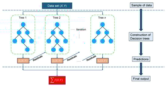
Figure 2.
The architecture of the XGBoost algorithm.
Following [67], the objective function that needs to be minimized at t-th iteration is:
where is the target value, is the prediction, l is a differentiable loss function, is the output of the new model at iteration t, and n is the number of training samples. The first term of Equation (10) measures how well the model perform on training data, and the second term is a regularization term that measures the complexity of the base learners (i.e., trees), to avoid overfitting. In Equation (11) T stands for the number of leaves in the tree, with leaf weights w, and , are regularization parameters. The task of optimizing this objective function can be simplified to minimizing a quadratic function, by using the second order Taylor expansion [70].
XGBoost is sensitive to hyperparameters and careful tuning is required to achieve good performance. This process can lead to pretty high optimization, particularly when working with large datasets. The model only accepts numerical values for processing. Additionally, the model’s complexity makes it less interpretable compared to simpler algorithms.
2.4. Long Short-Term Memory (LSTM)
Long Short-Term Memory (LSTM) networks represent an enhanced version of Recurrent Neural Networks (RNNs) [71], engineered to hold onto information from previous data for extended periods. They are designed for processing sequential data. LSTMs adeptly address the challenge of long-term dependencies through the incorporation of three gating mechanisms and a dedicated memory unit. They were first introduced by Hochreiter and Schmidhuber in 1997 [72] marking a milestone in deep learning. In many cases it is very important to know the previous time steps for a long length, in order to obtain a correct prediction of the outcome in each problem. This type of networks try to solve the “vanishing gradients” problem [73] (i.e., the loss of information during training that occurs when gradients become extremely small and extend further into the past), which remains the main problem in RNN’s. At its core, LSTM consists of various components, including gates and cell state (also referred as the memory of the network), which collectively enable it to selectively retain or discard information over time. In a LSTM network there are three gates as depicted in Figure 3, and the back-propagation algorithm is used to train the model. These three gates and the cell state can be described as follows:
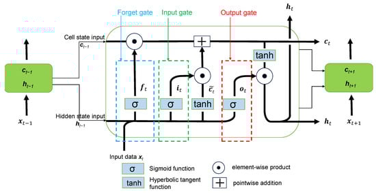
Figure 3.
Illustration of the LSTM cell architecture, for the time instances , with the corresponding gates (Adapted from [74]).
- Input gate: decides how valuable the current input is for solving the task, thus choosing the inflow of new information, selectively updating the memory cell. This gate uses the hidden state at former time step and current input to update the input gate with the following equation:
- Forget gate: decides which information from the previous cell state is to be discarded, allowing the network to prioritize relevant information. This is determined by the sigmoid function. Specifically, it takes the previous hidden state as well as the current input and outputs a number between 0 (meaning this will be skipped) and 1 (meaning this will be utilized), for each number of the cell state . The output of the forget gate can be expressed as:
- Output gate: regulates the information that the network outputs, refining the data stored in the memory cell. It decides what the next hidden state should be and this is achieved through the output vector . The output of this gate is described by the equation:
- Cell state: the long-term dependencies are encoded in the cell states and in this way the problem of “vanishing gradients” can be avoided. Cell state at current time step updates the former by taking into account the candidate cell state , representing the new information that could be added to the cell state, the input vector and the forget vector . Cell states updated values are as follows:
Final output of the LSTM has the form:
To summarize, Equations (12)–(17) express the mathematical calculations that are performed sequentially in the LSTM model, where , , are the input gate, forget gate and output gate vectors respectively, with subscript t indicating the current time step; , , represent weight matrices for connecting input, forget, and output gates with the input , respectively; , , denote weight matrices for connecting input, forget, and output gates with the hidden state ; , , are input, forget, and output gate bias vectors, respectively; the candidate cell state and the current cell state. Two activation functions is being used with and stands for sigmoid function and hyperbolic tangent function respectively. Finally ⊙ operation is the element-wise or Hadamard product and + operation is simply pointwise addition.
LSTMs in general have huge computational complexity, especially when dealing with long sequences. Additionally, like other machine and deep learning models, they are prone to overfitting when there is insufficient training data. Learning dependencies over very long sequences is challenging due to the aforementioned vanishing (or exploding) gradient problem. Lastly, the hyperparameter tuning coupled with limited interpretability further adds to model’s drawbacks.
2.5. Transformer-Based Model (Informer)
First off, an initial examination of transformer models is imperative for our investigation. The characteristic feature of transformers is the so-called self-attention mechanism, enabling the model to weigh different parts of the input sequence differently based on their relevance. This attention mechanism allows transformers to capture long-range dependencies efficiently, breaking the sequential constraints of traditional models like LSTMs. The transformer architecture consists of encoder and decoder layers, each comprised of multi-head self-attention mechanisms and feedforward neural networks. The encoder processes the input sequence using self-attention mechanisms to extract relevant features. The decoder then utilizes these features to generate the output sequence, incorporating both self-attention and encoder-decoder attention mechanisms for effective sequence-to-sequence tasks. The use of positional encoding provides the model with information about the position of input tokens in the sequence. Parallelization becomes a strength, as transformers can process input sequences in parallel rather than sequentially, significantly speeding up training and inference.
The Informer model, which was proposed by Zhou et al. (2021) [54], is a deep artificial neural network, and more specifically an improved Transformer-based model, that aims to solve the Long Sequence Time-series Forecasting (LSTF) problem [54]. This problem requires high prediction capability to capture long-range dependence between inputs and outputs. Unlike LSTM, which relies on sequential processing, transformers, and consequently Informer, leverage attention mechanisms to capture long-range dependencies and parallelize computations. The key feature lies in self-attention, allowing the model to weigh input tokens differently based on their relevance to each other, enhancing its ability to capture temporal dependencies efficiently. The rise in the application of transformer networks have emphasized their potential in increasing the forecasting capability. However, some issues concerning the operation of transformers, such as the quadratic time complexity (), the high memory usage and the limitation of the encoder-decoder architecture, make up transformer to be unproductive in problems when dealing with long sequences. Informer addresses those issues of the “vanilla” transformer [34] and trying to resolve them, by applying three main characteristics [54]:
- ProbSparse self-attention mechanism: a special kind of attention mechanism (ProbSparse—Probabilistic Sparsity) which achieves in time complexity and memory usage, where L is the length of the input sequence.
- Self-attention distilling: a technique that highlights the dominant attention making it effective in handling extremely long input sequences.
- Generative style decoder: a special kind of decoder that predicts long-term time series sequences with one forward pass rather than step-by-step, which drastically improves the speed of forecast generation.
Informer model preserves the classic transformer architecture, i.e., encoder-decoder architecture, while at the same time aiming to solve LSTF problem. The LSTF problem, that Informer is trying to solve, has an sequence input at time t, following the formulation of [75]:
and the output or target (predictions) is the corresponding sequence of vectors:
where , are input and output series of vectors at a specific time t, and are the input and output number of elements, respectively. LSTF encourage a longer enough output length , than usual forecasting cases. Informer supports all forecasting tasks (e.g., multivariate predict multivariate, multivariate predict univariate etc.), where are feature dimensions of input and output, respectively.
The structure of Informer model is illustrated in Figure 4, wherein three main components are distinguished: encoder layer, decoder layer and prediction layer. Encoder mainly handles longer sequence inputs by using sparse self-attention, an alternative to the traditional self-attention method. The trapezoidal component refers to the extracted self-attention operation, which significantly reduces the network’s size. The component between multi-head (i.e., a module for attention mechanisms which is often applied several times in parallel) ProbSparse attention, indicates self-attention distilling blocks (presented with light blue), that lead to concatenated feature map. On the other side, the decoder deals with input from the long-term sequence, padding target elements to zero. This procedure computes an attention-weighted component within the feature graph, resulting in the prompt generation of these elements in an efficient format.
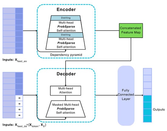
Figure 4.
Informer model structure (Adapted from ’Informer: Beyond Efficient Transformer for Long Sequence Time-Series Forecasting’, Zhou et al. [54]).
The ProbSparse (i.e., Probabilistic Sparsity) self-attention mechanism reduces the computation cost of self-attention drastically, while maintaining its effectiveness. Essentially, instead of Equation (20), Informer uses Equation (21) for the calculation of attention. The core concept of the attention mechanism revolves around computing attention weights for each element in the input sequence, indicating their relevance to the current output. This process begins by generating query (q), key (k), and value (v) vectors for each element in the sequence, where the query vector represents the current network output state, and the key and value vectors correspond to the input element and its associated attribute vector, respectively. Subsequently, these vectors are utilized to calculate attention weights through a scaled dot-product relation, measuring the similarity between the vectors. Figure 5 provides an overview of the attention mechanism’s architecture, where MatMul stands for matrix multiplication, SoftMax is the normalized exponential function for converting numbers into a probability distribution, and Concat for concatenation. The function that summarises attention mechanism can be written as [34]:
where Q, K, V are the input matrices of the attention mechanism. The dot-product of query q and key k is divided by the scaling factor of , with d representing the dimension of query and key vectors (input dimension). The significant difference between Equations (20) and (21) is that keys K are not linked to all possible Q queries but to the u most dominant ones, resulting in the matrix (which is obtained by the sparse probability distribution of Q).
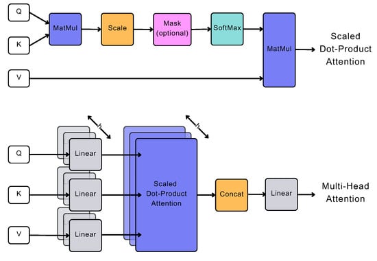
Figure 5.
Visualization of attention mechanism (Adapted from ‘Attention Is All You Need’, Vaswani et al. [34]).
An empirical approach is proposed for effectively measuring query sparsity, which is calculated by a method similar to Kullback–Leibler divergence. For each (query) and in the set of keys K, there is the bound [54]. Therefore, the proposed max-mean measurement is as follows:
If the query achieves a higher ), its attention probability p becomes more “diverse” and is likely to include the dominant dot-product pairs in the header field of the long-tail self-attention distribution.
The distribution of self-attention scores follows a long-tail distribution, with “active queries” positioned at the upper end of the feature map within the “head” scores, while “lazy queries” reside at the lower end within the “tail” scores. The preceding is illustrated in Figure 6. The ProbSparse mechanism is tailored to prioritize the selection of “active” queries over “lazy” ones.
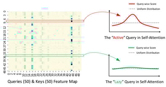
Figure 6.
Illustration of ProbSparse Attention (Source: [76]).
The encoder aims to capture the long-range dependencies within the lengthy sequence of inputs, under the constraint of using memory. Figure 7 is depicting model’s encoder. The process of self-attention distilling serves to assess the dominant features and generate a consolidated map of self-attention features for the subsequent level. Essentially, it involves simplifying the complex self-attention mechanism of the transformer model into simpler and smaller form, suitable for integration into the Informer model.

Figure 7.
Informer’s encoder architecture (Adapted from [54]).
As distinguished in Figure 7 encoder contains enough attention blocks, convolution layers (Conv1d) and max pooling layers (MaxPool), to encode the input data. The copies of the main stack (Attention Block 1) with continuously decreasing inputs by half, increase the reliability of the distilling operation. The process continues by reducing to of the original length. At the end of the encoder, all feature maps are concatenated to direct the output of the encoder directly to the decoder.
The purpose of the distillation operation is to reduce the size of the network parameters, giving higher weights to the dominant features, and produce a focused feature map in the subsequent layer. The distillation process from the j-th layer to the -th layer is described by the following procedure:
where represents the attention block, Conv1d(·) performs an 1-D convolutional filters with the ELU(·) activation function [77].
The structure of the decoder does not differ greatly from that published by Vaswani et al. [34]. It is capable of generating large sequential outputs through a single forward pass process. As shown in Figure 4, it includes two identical multi-head attention layers. The main difference is the way in which the predictions are generated through a process called generative inference, which significantly speeds up the long-range prediction process. The decoder receives the following vectors:
where is the start token (i.e., parts of input data), is a placeholder for the target sequence (set to 0). Subsequently, the masked multi-head attention mechanism adjusts the ProbSparse self-attention computation by setting the inner products to , thereby prohibiting each position from attending to subsequent positions. Finally, a fully connected layer produces the final output, while the dimension of the output depends on whether univariate or multivariate prediction is implemented.
Although Informer reduces time complexity compared to vanilla Transformers, it can still be resource-intensive, requiring significant memory and processing power for very large datasets. As a deep learning model, its performance depends on the quality and quantity of the training data, and it also requires careful hyperparameter tuning, which could be time-consuming and may need specific domain knowledge.
2.6. Evaluation Metrics
To assess the effectiveness of the different models accurately, this paper engages Mean Squared Error (MSE), Root Mean Squared Error (RMSE), Mean Absolute Error (MAE), Mean Absolute Percentage Error (MAPE) and Nash-Sutcliffe Efficiency (NSE) coefficient as evaluation metrics. In some cases, the coefficient of determination was also determined. The formulas for calculating these metrics are provided below.
where is the i-th observed value; is the corresponding forecasted value; is the mean of the y observed values; is the predicted values from the statistical model (linear regression model) inferred from the observed values; and n the number of total data points for .
3. Analysis and Results (Case Study 1: River Test)
3.1. Study Area
The study area centers on the River Test [78] (Figure 8), situated in Hampshire, southern England. It rises at Ashe close to Basingstoke, it spans approximately 64 km2, flowing southwards until it meets Southampton Water. The River Test is an important watercourse known for its ecological diversity, historical and hydrological significance. Notably, it encompasses a significant biological area designated as a Special Scientific Interest, spanning 438 hectares (ha).
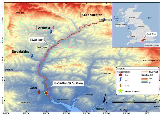
Figure 8.
Study area.
3.2. Data
The hydroclimatic data were collected, stored, processed and consolidated, by national data centres in England. In particular, data from The CEDA Archive [79], Defra [80], and the National River Flow Archive [81] were utilized. Dataset contains 12 features, among which flow from river stations and climate data of the region, i.e., precipitation and temperature across diverse points within the region of Hampshire in England. The dataset comprises 41 years of daily observations spanning from 1980 to 2021, totaling 15,341 values (slightly fewer in certain attributes). Figure 9 presents the first 20 rows of the data in tabular format, displaying all their attributes, while Table 1 provides a description of these characteristics. Table 2 shows the medatada information about the stations of the dataset.
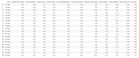
Figure 9.
River Test dataset format.

Table 1.
Description of data features.
Table 2.
Metadata of stations of the dataset.
During the data preprocessing stage, we conducted checks to identify any erroneous values, temporal gaps or potential outliers in the data. In this study we focus on streamflow forecasting, while the flow_Broadlands column was selected for the method application. This column represents the measured flow in the Broadlands area (Figure 8). The fluctuation in flow is closely associated with flooding events, making this data characteristic particularly important.
The streamflow measurements consists of 15,225 values from 1 January 1980 to 6 September 2021. We split the data into training, validation, and testing sets using a ratio of 0.7:0.1:0.2, a fairly common splitting scheme. Approximately, the initial 33 years were used for model training, with the remaining data allocated for testing. Figure 10 illustrates the time series of the station streamflow, with the training (train), validation (val) and testing (test) data split indicated.
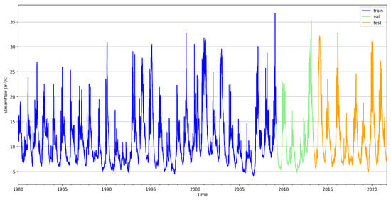
Figure 10.
River Test streamflow time series of Broadlands station.
In this particular case study we aim to forecast streamflow time series at the Broadlands station using various forecast horizons. The selected forecast horizons include 2, 10, 20, 40, 60, 80, 100, and 168 days. Five different models were employed: a Hurst–Kolmogorov stochastic model (SB), a common time series model (ARIMA), and machine and deep learning networks (XGBoost, LSTM and Informer). All analyses and code development were conducted in Python 3.10.12, utilizing relevant libraries. The computational resources of Google Colab, specifically the NVIDIA Tesla K80 with 12 GiB VRAM, were leveraged to ensure optimal conditions for training deep neural networks.
3.3. Model Architectures
3.3.1. SB
For this application, the stochastic benchmark model, described in Section 2.1, was chosen over a naive model. The naive approach assumes that future values in a time series will mirror the most recent observed value, or the mean of all values of the time series. In contrast, the SB model determines the precise number of past terms to consider and computes a representative average for the forecast horizon at hand. This model serves as a benchmark for comparison against more sophisticated forecasting models.
In order to find the required conditions (in our case days) to be taken into account regarding the forecast horizon, it is necessary to calculate the Hurst coefficient H, which is approximated by the climacogram. Figure 11 shows the climacogram of the time series of streamflow at Broadlands station. For simplicity, only the long-term dependence was considered (highlighted with orange in Figure 11), rather than the entire climacogram. This resulted in a coefficient of H = 0.7, which simplifies things and equations of Section 2.1 are directly applicable. Utilizing Equation (8) we compute the required , based on given and H. Table 3 summarizes those combinations of , .

Figure 11.
Empirical climacogram of streamflow at Broadlands station.
Table 3.
Ratio of terms (in days) of past and future .
3.3.2. ARIMA
By monitoring the AIC metric values across different parameter combinations, as well as their corresponding time, it was determined that the optimal parameters for the ARIMA model are ARIMA(3,1,3). For this specific model the AIC was found to be AIC = 34,941.93 with a corresponding computational time of 9.7 s.
3.3.3. XGBoost
Using the XGBoost Python package 2.1.1, we constructed a forecasting model by first generating features based on the date and incorporating lagged values from the time series, to effectively model time-dependent relationships in the data. To ensure robust model performance, we employed cross-validation in our evaluation process. After optimizing the model through Grid Search, we finalized the hyperparameters, which are detailed in Table 4.
Table 4.
XGBoost model Hyperparameters.
3.3.4. LSTM
The LSTM model was constructed using the PyTorch library 2.1.0, a widely used tool for deep learning tasks. During training, the time series data was utilized, and fixed-length sequences were generated after zero mean and unit variance normalization. Sequentially, each sequence was fed into the LSTM model individually, with the immediate subsequent value also recorded, using a sliding window method. Sliding window method divides training data into overlapping windows of fixed size. Each window serves as an input sequence for the model, with the target being the future values of the time series [82]. Through testing and experimentation with different architectures, the optimal hyperparameters and network architecture were identified, as summarized in Table 5. This iterative process involved adjusting and refining the model to achieve the best performance.
Table 5.
LSTM model Hyperparameters.
3.3.5. Informer
The final and main model examined in this study is the transformer-based Informer model, which was also implemented using PyTorch library 2.1.0. Following data partitioning into training, validation, and test sets, normalization is applied, and the data is segmented into input and target subsequences, as previously, using the sliding window method. Data were normalized such that the mean is 0 and the standard deviation is 1 (StandardScaler). The input subsequences are then passed through the encoder to the decoder, where future values of the time series are predicted. Table 6 outlines the model architecture, excluding details on the encoder input sequence length and prediction sequence length. Through an iterative fine-tuning process involving various combinations of input and prediction sequences, optimal values, as presented in Table 7, were determined.
Table 6.
Informer model Hyperparameters.
Table 7.
Combinations of input sequence length and prediction length of Informer model.
3.4. Results and Comparison
As previously mentioned, the forecast horizon spans from 2 to 168 days. Table 8 provides a detailed overview of the performance metrics, including NSE, RMSE, MAE, and MAPE, for each of the forecast horizons, across all models. For each forecast horizon, the best scores are emphasized in bold. Figure 12 provides a comprehensive and straightforward representation of the data presented in the corresponding table, through a bar chart depicting evaluation metrics. Furthermore, Figure 13 depict the predicted and ground truth values in corresponding prediction window.
Table 8.
Models results of streamflow forecasting on River Test. The best result for each metric at each forecast horizon is highlighted in bold.
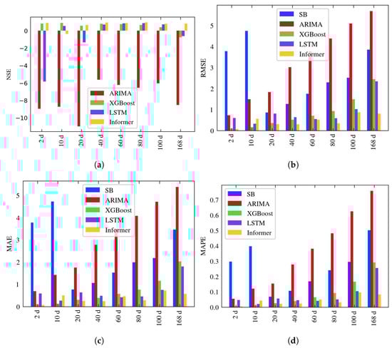
Figure 12.
Bar chart presenting the evaluation metric results. In subfigure (a), the SB method is excluded due to its high error values, which affected effective visualization. (a) NSE metric. (b) RMSE metric. (c) MAE metric. (d) MAPE metric.
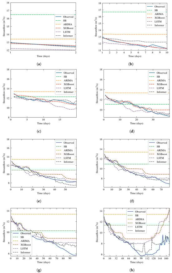
Figure 13.
Prediction results of all five models compared with ground truth across all prediction windows. (a) Forecast horizon = 2 days. (b) Forecast horizon = 10 days. (c) Forecast horizon = 20 days. (d) Forecast horizon = 40 days. (e) Forecast horizon = 60 days. (f) Forecast horizon = 80 days. (g) Forecast horizon = 100 days. (h) Forecast horizon = 168 days.
Insights can be derived from the findings presented in Table 8. The machine and deep learning models exhibit superior performance compared to both the naive stochastic approach and the statistical ARIMA model, which struggles to fully grasp the complex dynamics of time series. The SB model displayed poor predictive capabilities, with extremely low NSE values. Meanwhile, XGBoost and LSTM demonstrates robust performance at the 10-day forecasting horizon, but its effectiveness diminished at longer time horizons. At the 10-day forecast horizon, XGBoost ranks as the highest-performing algorithm; on the other hand LSTM has the lowest MAE value on 60-day forecast. Overall, the Informer model stands out as the top performer. Remarkably, the Informer model significantly improves the results, with the prediction error gradually and smoothly increasing as the prediction horizon extends. This underscores the Informer’s effectiveness in improving prediction capabilities for long-range forecasting tasks. The Informer’s performance, as measured by the MAPE metric, does not surpass 10%, while the NSE coefficient achieves 0.8 at the longest horizon, demonstrating a high level of accuracy.
As noted in the model comparison, the Informer model excels, having the best performance. Figure 14 presents the Informer model’s outcomes in a scatter plot displaying predicted streamflow values. The solid blue line in the plot represents the ideal estimation, where if each prediction point of the model matched the actual observed value. Overall, Informer model demonstrates good performance, with the trend line exhibiting a coefficient of determination () of 0.91. However, weaker performance is noted at lower values, corresponding to local minima in our context.

Figure 14.
Scatter plot of predicted streamflow values from the Informer model in the River Test.
4. Analysis and Results (Case Study 2: Examining the Performance of the Informer Model across Numerous Rivers)
4.1. Study Area
The selected study area for evaluating the Informer performance across a substantial number of time series (>100) covers a wider area of the United Kingdom, where the previous case study belongs as well.
Given its varied topography and extensive river networks, the UK frequently witnesses devastating flooding incidents with far-reaching consequences. This study centers on the rivers of the UK, aiming to devise and assess a deep learning-based method for forecasting flood events, and more specifically the Informer model.
A key factor motivating the selection of this study area is the extensive database maintained by the United Kingdom, known as the National River Flow Archive (NRFA) [81], which systematically gathers and manages data on river flow from numerous gauging stations across the entire country. This database serves as a fundamental resource for the current investigation. Figure 15 depicts the extensive coverage of gauging stations within the NRFA database, along with the corresponding river networks.
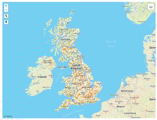
Figure 15.
Map of the UK with the locations of available stations from the NRFA database (Source: https://nrfa.ceh.ac.uk/data/search (accessed on 10 February 2023)).
4.2. Data
As already mentioned, the data were obtained from the NRFA database [81] and are available online. Similar to the prior study, this analysis focuses on time series data of river streamflow, aiming to forecast for a specific horizon. Accessing this database allows for straightforward searches, leveraging filters based on specific criteria relevant to individual research needs (e.g., real-time data availability, location etc.). In this particular study, the selection was primarily based on three criteria:
- The availability of daily streamflow data.
- The time series should span a long period (i.e., >20 years).
- The data should be continuous without missing values, with a completeness rate exceeding 95%.
This analysis resulted in a collection of 112 data stations, with their respective geographical locations illustrated in Figure 16. The dataset collected represents a broad spectrum of river morphologies, hydroclimate conditions, and varying amounts of historical data.
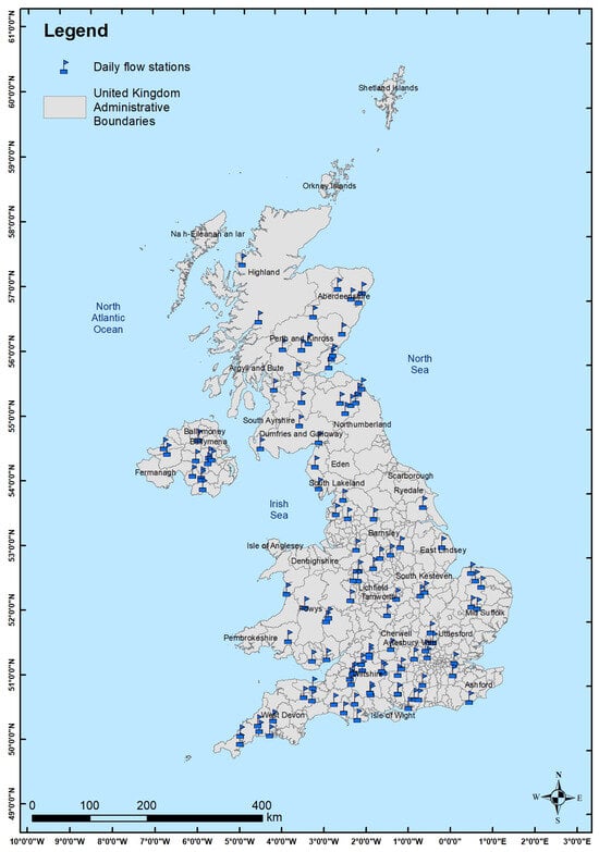
Figure 16.
Geographical distribution of the 112 stations used for forecasting.
4.3. Informer Architecture
The evaluation using the Informer model was conducted uniformly across all time series with identical architecture and forecast horizon (30 days). Since the study’s aim wasn’t to fine-tune forecast results for each individual river, conducting a thorough hyperparameters search on a river-by-river basis was considered unnecessary, computationally expensive and time-consuming. Based on the case study presented in Section 3, we identified the optimal architecture tailored to the specified forecast horizon. Thus, the selection of input and output sequences mirrored that of the previous River Test study and remained consistent. Following data split into training, validation, and testing sets (maintaining a 70:10:20 ratio), normalization and segmentation into input and target subsequences were performed as previously. Table 9 outlines the details on the model architecture employed.
Table 9.
Informer model Hyperparameters, used in the second case study for the 112 stations.
4.4. Results
For the 30-day forecast horizon and utilizing the same architecture, the Informer model was trained to forecast the river flow for each station. It’s important to highlight that this approach isn’t ideal for deep learning-based forecasting tasks, as each time series should ideally be individually treated and optimized. However, addressing such a significant quantity of time series in this manner demands significant computational resources and time. Hence, for this specific scenario, the investigation focused on evaluating the model’s performance using a fixed network architecture.
Figure 17 summarises the prediction results of all 112 stations in a single scatter plot between observed and estimated flows. The figure also provides the optimal prediction (red solid line), where the forecast coincides with the ground truth. However, the trend line of the predictions (blue dashed line) exhibits a coefficient of determination = 0.4, implying poor model performance. Figure 17 also shows the box plot illustrating the MAPE performance metrics. Specifically, for every 30-day forecast of each time series, the MAPE metric was computed once. The sum of these errors, for each time series, is plotted in the box plot. The diagram depicts the moderate performance of the Informer network, characterized by a median value of 0.5 or 50%.
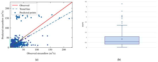
Figure 17.
(a) Scatter plot of predicted Informer model values and (b) box plot of the MAPE error metric between estimated and observed streamflow, examined at 112 stations.
To examine the underperformance of the model, we analysed the scores of loss functions across the three subdivisions of all time series (i.e., train, validation and test set), relative to the structure of the time series, as represented by climacograms. Figure 18 displays all the empirical climacograms. The entire 112 climacograms were sorted according to their slope, and subsequently, their respective losses on the train, validation, and test sets were assigned to each one. The results of the earlier investigation are plotted in Figure 19.
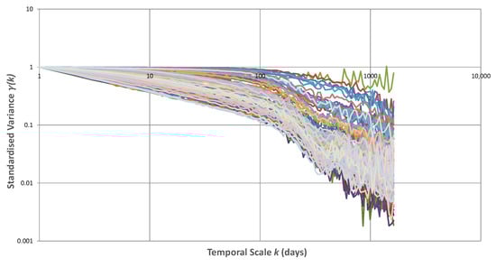
Figure 18.
Empirical climacograms of the 112 daily streamflow time series used in the analysis.
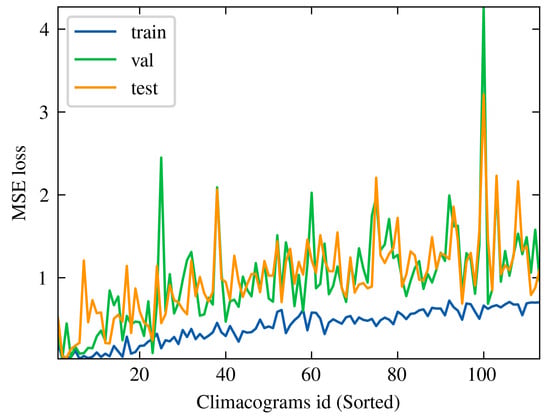
Figure 19.
Informer performance compared with climacograms. On horizontal axis each climacogram is sorted based on slope, in ascending order. Climacogram with id near to zero indicates higher H value, which decreases as we move towards the right of the axis.
5. Discussion and Future Directions
In the past few years, transformer network and the variations of its architecture have been extensively applied across many domains [35]. Although the high popularity they receive, their usage in hydrology and streamflow forecasting is still in its early stages and remains relatively underdeveloped. In the above sections we tried to make some insights about streamflow forecasting with a transformer-based model. i.e., Informer. We utilized real-world data to assess the performance of the models, evaluating results with widely used metrics— and . When some studies analyse flood prediction with transformer models, they typically rely on data from only one or two stations to generate their results (e.g., [53,58,83]). In contrast, we also make a case study where we focus on the Informer model and its performance on more than 100 river streamflow stations.
In the initial application, where data from River Test were analysed, we compared the Informer model, the LSTM model, the XGBoost model, the ARIMA model and the Hurst-Kolmogorov stochastic approach [84]. Data include daily streamflow of Broadlands station and the chosen forecast horizons were 2, 10, 20, 40, 60, 80, 100, and 168 days. Machine and deep learning approaches have the best results, with the Informer showing its superiority over LSTM and XGBoost—especially for long-term prediction (Figure 13). It should be noted that SB and ARIMA models could have better results if the seasonality was explicitly modeled. Stochastic approach could replace the classic baseline models in hydrology and especially in forecasting problems, as it is theoretically authenticated. Based on our results (Figure 14) Informer model has pretty good performance with a coefficient of 0.91. The optimization task in transformer networks is a pretty challenging work, due to their complex architecture and the vast number of hyperparameters involved. This process is time consuming, requires computational resources and cautious fine-tuning to balance performance and efficiency.
Due to this extensive procedure, we chose to universally perform Informer model in the second case study, with the same hyperparameters. This involved using a large dataset containing 112 river basins and the model used the best set of hyperparameters, as revealed from the first implementation for a forecast horizon of 30 days. The upper had a totally different performance, resulting a coefficient of determination 0.4 for all the stations (Figure 17a). Bad behaviour of Informer is represented also by the boxplot in Figure 17b, where for each station is calculated MAPE error. This case arises with a median value of 50%. An interesting insight of this large analysis is the fact that model performance is related to climacogram of the time series. Climacogram is a high effective stochastic tool [61] for detecting the long-term changes, thereby providing a better understanding of a process. We analysed stations that provide a wide range of different characteristics, as illustrated in Figure 18. We then tracked the MSE loss function values across all three subsets: training, validation, and test sets. An upward trend in MSE loss was observed as the Hurst coefficient H decreased. Figure 19 shows this outcome, where on x-axis each climacogram is sorted based on the slope, in ascending order. Thus, climacograms with id near zero indicates a higher H value, which decreases as we move towards the right of the axis. From one point of view this observation is a bit anticipated, since a stochastic process with high Hurst value is less unpredictable in short-term prediction [85]. The situation is being reversed in long-range prediction, where a time series with high Hurst coefficient has bigger uncertainty. In our case we had 30 days forecast horizon, which corresponds to short-term forecasting and results verify the above findings.
The scope of this study may be increased, leading to a major improvement in the methods employed in the current work to improve the performance and applicability of the models. To begin with, the development and evaluation of other transformer-based models and networks for the problem of streamflow forecasting should be considered. This great popularity they receive in other topics, such as natural language processing, suggests their likely utility in flood prediction as well. Additionally, in order to improve forecasts, the exploitation of other flood-related variables (e.g., temperature, rainfall, etc.) in the context of multivariate forecasting needs to be looked into. Another important aspect is quantifying the uncertainty of such models and addressing it through probabilistic forecasting. Moreover, the investigation of the performance of transformer ensemble modelling with statistical, stochastic, or other deep learning networks and the evaluation of models by implementing real-time predictions for immediate comparison can bring useful knowledge. Similarly to the approach taken in this research, an analysis of the impact that time series characteristics may have on the performance of the Informer model (and beyond) should be conducted [86], along with the identification of techniques or transformations to address any potential issues that arise. On top of that, post-processing techniques might boost the model’s results. Lastly, but equally important, is the attempt to interpret the operation of deep learning models (Interpretable AI) [87] and explain their results or the decisions made (Explainable AI) [88]. A way to achieve this is by incorporating models like PINNs, which integrate the underlying physics of the problem being addressed.
6. Summary and Conclusions
In this work, we study the contribution of deep learning networks to the prediction of time series related to flood events. Special emphasis was placed on modern deep learning tools such as transformer networks and in particular the Informer model. We executed two applications, where in the first one we compared five models on streamflow data from the River Test in England. Comparisons with more traditional deep learning networks (LSTM), machine learning model (XGBoost) and time series model (ARIMA) were included, along with the introduction of a naive Hurst–Kolmogorov stochastic approach for predictive modeling as a reference model. A distinct examination was conducted, as a secondary case study on the Informer model, evaluating its performance across a multitude of rivers in the UK. The analysis and processing of the applications led to some conclusions, which are summarised below:
- The stochastic approach is simple and theoretically substantiated on stochastic processes, suitable for use as a reference model.
- The technology of transformer based models shows great potential for improving the accuracy of time series forecasting models for both short-term and long-term sequences, when fine-tuning model’s hyperparameters for each time series individually.
- The Informer model significantly decreases the time complexity and memory requirements compared to “vanilla” transformers. However the training and learning process remains a challenging and time-consuming task.
- Regarding the first application, the Informer model demonstrated superior performance in the River Test application, outperforming the other models. The ARIMA statistical model struggled to capture the complex patterns in the time series, when seasonality is not explicitly modeled. The XGBoost and LSTM network performed well for short-term forecasting, which is not the case for the long-term prediction, whereas Informer delivered better results.
- In the second case, exploring the Informer model across numerous rivers revealed that the performance of the model can be influenced by the structure of the time series data.
- Transformers come with drawbacks such as computational complexity, limited interpretability, and limited scalability. Therefore, each time series needs to be addressed and assessed independently.
Floods are a major problem nowadays, and accurate forecasting helps in dealing with them. However, it remains a challenging task to solve. Overall, the transformer’s architecture is notably promising in addressing complex temporal patterns and concepts. Nevertheless, as has been noted, computational complexity and scalability pose limitations that need to be addressed. More analysis on those kinds of networks should be explored in future hydrologic research. Future research should focus on optimizing these models to enhance efficiency and interpretability, ensuring their practical applicability in flood forecasting, as well as exploring the impact of different hyperparameters on their performance.
Author Contributions
Conceptualization, N.T.; methodology, N.T.; software, N.T.; validation, N.T.; formal analysis, N.T.; investigation, N.T., D.K, T.I. and P.D.; resources, N.T.; data curation, N.T.; writing—original draft preparation, N.T.; writing—review and editing, N.T. and D.K.; visualization, N.T.; supervision, N.T., D.K., T.I. and P.D.; project administration, N.T., D.K., T.I. and P.D. All authors have read and agreed to the published version of the manuscript.
Funding
This research received no external funding.
Data Availability Statement
The data used, were retrieved from UK National River Flow Archive and are available online for free (https://nrfa.ceh.ac.uk/data/search (accessed on 10 February 2023)). The data are provided under the terms and conditions specified by the archive.
Conflicts of Interest
The authors declare no conflict of interest.
References
- Yu, Q.; Wang, Y.; Li, N. Extreme Flood Disasters: Comprehensive Impact and Assessment. Water 2022, 14, 1211. [Google Scholar] [CrossRef]
- Yan, Z.; Li, M. A Stochastic Optimization Model for Agricultural Irrigation Water Allocation Based on the Field Water Cycle. Water 2018, 10, 1031. [Google Scholar] [CrossRef]
- Nearing, G.S.; Kratzert, F.; Sampson, A.K.; Pelissier, C.S.; Klotz, D.; Frame, J.M.; Prieto, C.; Gupta, H.V. What Role Does Hydrological Science Play in the Age of Machine Learning? Water Resour. Res. 2021, 57, e2020WR028091. [Google Scholar] [CrossRef]
- Kumar, V.; Kedam, N.; Sharma, K.V.; Mehta, D.J.; Caloiero, T. Advanced Machine Learning Techniques to Improve Hydrological Prediction: A Comparative Analysis of Streamflow Prediction Models. Water 2023, 15, 2572. [Google Scholar] [CrossRef]
- Liang, J.; Li, W.; Bradford, S.; Šimůnek, J. Physics-Informed Data-Driven Models to Predict Surface Runoff Water Quantity and Quality in Agricultural Fields. Water 2019, 11, 200. [Google Scholar] [CrossRef]
- Wang, Z.-Y.; Qiu, J.; Li, F.-F. Hybrid Models Combining EMD/EEMD and ARIMA for Long-Term Streamflow Forecasting. Water 2018, 10, 853. [Google Scholar] [CrossRef]
- Yang, M.; Wang, H.; Jiang, Y.; Lu, X.; Xu, Z.; Sun, G. GECA Proposed Ensemble-KNN Method for Improved Monthly Runoff Forecasting. Water Resour. Manag. 2020, 34, 849–863. [Google Scholar] [CrossRef]
- Ni, L.; Wang, D.; Singh, V.P.; Wu, J.; Wang, Y.; Tao, Y.; Zhang, J. Streamflow and rainfall forecasting by two long short-term memory-based models. J. Hydrol. 2020, 583, 124296. [Google Scholar] [CrossRef]
- Ghimire, S.; Yaseen, Z.M.; Farooque, A.A.; Deo, R.C.; Zhang, J.; Tao, X. Streamflow prediction using an integrated methodology based on convolutional neural network and long short-term memory networks. Sci. Rep. 2021, 11, 17497. [Google Scholar] [CrossRef]
- Qi, X.; de Almeida, G.A.; Maldonado, S. Physics-informed neural networks for solving flow problems modeled by the 2D Shallow Water Equations without labeled data. J. Hydrol. 2024, 636, 131263. [Google Scholar] [CrossRef]
- Digital Science. Dimensions AI: The Most Advanced Scientific Research Database; Dimensions: Reading, UK, 2018; Available online: https://app.dimensions.ai/discover/publication (accessed on 2 June 2024).
- Box, G.E.P.; Jenkins, G.M. Time Series Analysis: Forecasting and Control; Holden-Day: San Francisco, CA, USA, 1970. [Google Scholar]
- Ab Razak, N.H.; Aris, A.Z.; Ramli, M.F.; Looi, L.J.; Juahir, H. Temporal flood incidence forecasting for Segamat River (Malaysia) using autoregressive integrated moving average modelling. J. Flood Risk Manag. 2016, 11, S794–S804. [Google Scholar] [CrossRef]
- Nourani, V.; Najafi, H.; Amini, A.B.; Tanaka, H. Using Hybrid Wavelet-Exponential Smoothing Approach for Streamflow Modeling. Complexity 2021, 2021, 6611848. [Google Scholar] [CrossRef]
- Valipour, M.; Banihabib, M.E.; Behbahani, S.M.R. Comparison of the ARMA, ARIMA, and the autoregressive artificial neural network models in forecasting the monthly inflow of Dez dam reservoir. J. Hydrol. 2013, 476, 433–441. [Google Scholar] [CrossRef]
- Valipour, M.; Banihabib, M.E.; Behbahani, S.M.R. Parameters Estimate of Autoregressive Moving Average and Autoregressive Integrated Moving Average Models and Compare Their Ability for Inflow Forecasting. J. Math. Stat. 2012, 8, 330–338. [Google Scholar] [CrossRef]
- Jozaghi, A.; Shen, H.; Ghazvinian, M.; Seo, D.-J.; Zhang, Y.; Welles, E.; Reed, S. Multi-model streamflow prediction using conditional bias-penalized multiple linear regression. Stoch. Environ. Res. Risk Assess. 2021, 35, 2355–2373. [Google Scholar] [CrossRef]
- Yaseen, Z.M.; El-shafie, A.; Jaafar, O.; Afan, H.A.; Sayl, K.N. Artificial intelligence based models for stream-flow forecasting: 2000–2015. J. Hydrol. 2015, 530, 829–844. [Google Scholar] [CrossRef]
- Ikram, R.M.A.; Ewees, A.A.; Parmar, K.S.; Yaseen, Z.M.; Shahid, S.; Kisi, O. The viability of extended marine predators algorithm-based artificial neural networks for streamflow prediction. Appl. Soft Comput. 2022, 131, 109739. [Google Scholar] [CrossRef]
- Noori, R.; Karbassi, A.R.; Moghaddamnia, A.; Han, D.; Zokaei-Ashtiani, M.H.; Farokhnia, A.; Gousheh, M.G. Assessment of input variables determination on the SVM model performance using PCA, Gamma test, and forward selection techniques for monthly stream flow prediction. J. Hydrol. 2011, 401, 177–189. [Google Scholar] [CrossRef]
- Papacharalampous, G.A.; Tyralis, H. Evaluation of random forests and Prophet for daily streamflow forecasting. Adv. Geosci. 2018, 45, 201–208. [Google Scholar] [CrossRef]
- Ni, L.; Wang, D.; Wu, J.; Wang, Y.; Tao, Y.; Zhang, J.; Liu, J. Streamflow forecasting using extreme gradient boosting model coupled with Gaussian mixture model. J. Hydrol. 2020, 586, 124901. [Google Scholar] [CrossRef]
- Szczepanek, R. Daily Streamflow Forecasting in Mountainous Catchment Using XGBoost, LightGBM and CatBoost. Hydrology 2022, 9, 226. [Google Scholar] [CrossRef]
- Chang, F.-J.; Chang, L.-C.; Chen, J.-F. Artificial Intelligence Techniques in Hydrology and Water Resources Management. Water 2023, 15, 1846. [Google Scholar] [CrossRef]
- Sahoo, B.B.; Jha, R.; Singh, A.; Kumar, D. Long short-term memory (LSTM) recurrent neural network for low-flow hydrological time series forecasting. Acta Geophys. 2019, 67, 1471–1481. [Google Scholar] [CrossRef]
- Zhao, X.; Lv, H.; Wei, Y.; Lv, S.; Zhu, X. Streamflow Forecasting via Two Types of Predictive Structure-Based Gated Recurrent Unit Models. Water 2021, 13, 91. [Google Scholar] [CrossRef]
- Shu, X.; Ding, W.; Peng, Y.; Wang, Z.; Wu, J.; Li, M. Monthly Streamflow Forecasting Using Convolutional Neural Network. Water Resour. Manag. 2021, 35, 5089–5104. [Google Scholar] [CrossRef]
- Dong, J.; Wang, Z.; Wu, J.; Cui, X.; Pei, R. A Novel Runoff Prediction Model Based on Support Vector Machine and Gate Recurrent unit with Secondary Mode Decomposition. Water Resour. Manag. 2024, 38, 1655–1674. [Google Scholar] [CrossRef]
- Wang, Z.; Xu, N.; Bao, X.; Wu, J.; Cui, X. Spatio-temporal deep learning model for accurate streamflow prediction with multi-source data fusion. Environ. Model. Softw. 2024, 178, 106091. [Google Scholar] [CrossRef]
- Salinas, D.; Flunkert, V.; Gasthaus, J.; Januschowski, T. DeepAR: Probabilistic forecasting with autoregressive recurrent networks. Int. J. Forecast. 2019, 36, 1181–1191. [Google Scholar] [CrossRef]
- Taylor, S.J.; Letham, B. Forecasting at Scale. Am. Stat. 2018, 72, 37–45. [Google Scholar] [CrossRef]
- Zou, Y.; Wang, J.; Peng, L.; Li, Y. A novel multi-step ahead forecasting model for flood based on time residual LSTM. J. Hydrol. 2023, 620, 129521. [Google Scholar] [CrossRef]
- Tyralis, H.; Papacharalampous, G.A. Large-scale assessment of Prophet for multi-step ahead forecasting of monthly streamflow. Adv. Geosci. 2018, 45, 147–153. [Google Scholar] [CrossRef]
- Vaswani, A.; Shazeer, N.; Parmar, N.; Uszkoreit, J.; Jones, L.; Gomez, A.N.; Kaiser, Ł.; Polosukhin, I. Attention is all you need. Adv. Neural Inf. Process. Syst. 2017, 30, 5998–6008. [Google Scholar]
- Wen, Q.; Zhou, T.; Zhang, C.; Chen, W.; Ma, Z.; Yan, J.; Sun, L. Transformers in Time Series: A Survey. In Proceedings of the International Joint Conference on Artificial Intelligence (IJCAI’23), Macao, China, 19–25 August 2023. [Google Scholar]
- Li, S.; Jin, X.; Xuan, Y.; Zhou, X.; Chen, W.; Wang, Y.X.; Yan, X. Enhancing the Locality and Breaking the Memory Bottleneck of Transformer on Time Series Forecasting. In Proceedings of the Annual Conference on Neural Information Processing Systems 2019, NeurIPS 2019, Vancouver, BC, Canada, 8–14 December 2019; Volume 32. [Google Scholar]
- Wu, N.; Green, B.; Ben, X.; O’Banion, S. Deep Transformer Models for Time Series Forecasting: The Influenza Prevalence Case. arXiv 2020, arXiv:2001.08317. [Google Scholar]
- Wang, S.; Li, B.Z.; Khabsa, M.; Fnag, H.; Ma, H. Linformer: Self-Attention with Linear Complexity. arXiv 2020, arXiv:2006.04768. [Google Scholar]
- Kitaev, N.; Kaiser, L.; Levskaya, A. Reformer: The Efficient Transformer. In Proceedings of the International Conference on Learning Representations, Addis Ababa, Ethiopia, 26 April–1 May 2020; Available online: https://openreview.net/forum?id=rkgNKkHtvB (accessed on 15 May 2023).
- Beltagy, I.; Peters, M.E.; Cohan, A. Longformer: The Long-Document Transformer. arXiv 2020, arXiv:2004.05150. [Google Scholar]
- Yang, L.; Koprinska, I.; Rana, M. SSDNet: State Space Decomposition Neural Network for Time Series Forecasting. In Proceedings of the 2021 IEEE International Conference on Data Mining (ICDM), Auckland, New Zealand, 7–10 December 2021; pp. 370–378. [Google Scholar] [CrossRef]
- Lim, B.; Arık, S.Ö; Loeff, N.; Pfister, T. Temporal Fusion Transformers for interpretable multi-horizon time series forecasting. Int. J. Forecast. 2021, 37, 1748–1764. [Google Scholar] [CrossRef]
- Wu, H.; Xu, J.; Wang, J.; Long, M. Autoformer: Decomposition Transformers with Auto-Correlation for Long-Term Series Forecasting. Proc. Adv. Neural Inf. Process. Syst. (NeurIPS) 2021, 34, 22419–22430. [Google Scholar]
- Cirstea, R.G.; Guo, C.; Yang, B.; Kieu, T.; Dong, X.; Pan, S. Triformer: Triangular, Variable-Specific Attentions for Long Sequence Multivariate Time Series Forecasting. arXiv 2022, arXiv:2204.13767. [Google Scholar]
- Shen, L.; Wang, Y. TCCT: Tightly-coupled convolutional transformer on time series forecasting. Neurocomputing 2022, 480, 131–145. [Google Scholar] [CrossRef]
- Liu, S.; Yu, H.; Liao, C.; Li, J.; Lin, W.; Liu, A.X.; Dustdar, S. Pyraformer: Low-complexity pyramidal attention for long-range time series modeling and forecasting. In Proceedings of the International Conference on Learning Representations, Virtual, 25–29 April 2022. [Google Scholar]
- Drouin, A.; Marcotte, É.; Chapados, N. Tactis: Transformer-attentional copulas for time series. In Proceedings of the 39th International Conference on Machine Learning, Baltimore, MD, USA, 17–23 July 2022; pp. 5447–5493. [Google Scholar]
- Zhou, T.; Ma, Z.; Wen, Q.; Wang, X.; Sun, L.; Jin, R. FEDformer: Frequency Enhanced Decomposed Transformer for Long-term Series Forecasting. In Proceedings of the 39th International Conference on Machine Learning, Baltimore, MD, USA, 17–23 July 2022; pp. 27268–27286. [Google Scholar]
- Shabani, A.; Abdi, A.; Meng, L.; Sylvain, T. Scaleformer: Iterative Multi-Scale Refining Transformers for Time Series Forecasting. arXiv 2022, arXiv:2206.04038. [Google Scholar]
- Zhang, Y.; Yan, J. Crossformer: Transformer utilizing cross-dimension dependency for multivariate time series forecasting. In Proceedings of the The Eleventh International Conference on Learning Representations, Kigali, Rwanda, 1–5 May 2023. [Google Scholar]
- Fayer, G.; Lima, L.; Miranda, F.; Santos, J.; Campos, R.; Bignoto, V.; Andrade, M.; Moraes, M.; Ribeiro, C.; Capriles, P.; et al. Temporal Fusion Transformer Deep Learning Model for Long-Term Streamflow Forecasting: A Case Study in the Funil Reservoir, Southeast Brazil. Knowl.-Based Eng. Sci. 2023, 4, 73–88. [Google Scholar]
- Ghobadi, F.; Kang, D. Improving long-term streamflow prediction in a poorly gauged basin using geo-spatiotemporal mesoscale data and attention-based deep learning: A comparative study. J. Hydrol. 2022, 615, 128608. [Google Scholar] [CrossRef]
- Liu, C.; Liu, D.; Mu, L. Improved Transformer Model for Enhanced Monthly Streamflow Predictions of the Yangtze River. IEEE Access 2022, 10, 58240–58253. [Google Scholar] [CrossRef]
- Zhou, H.; Zhang, S.; Peng, J.; Zhang, S.; Li, J.; Xiong, H.; Zhang, W. Informer: Beyond Efficient Transformer for Long Sequence Time-Series Forecasting. Proc. AAAI Conf. Artif. Intell. 2021, 35, 11106–11115. [Google Scholar] [CrossRef]
- Shang, J.; Zhao, B.; Hua, H.; Wei, J.; Qin, G.; Chen, G. Application of Informer Model Based on SPEI for Drought Forecasting. Atmosphere 2023, 14, 951. [Google Scholar] [CrossRef]
- Yang, Z.; Liu, L.; Li, N.; Tian, J. Time Series Forecasting of Motor Bearing Vibration Based on Informer. Sensors 2022, 22, 5858. [Google Scholar] [CrossRef]
- Huang, X.; Jiang, A. Wind Power Generation Forecast Based on Multi-Step Informer Network. Energies 2022, 15, 6642. [Google Scholar] [CrossRef]
- Wei, H.; Wang, Y.; Liu, J.; Cao, Y. Monthly Runoff Prediction by Combined Models Based on Secondary Decomposition at the Wulong Hydrological Station in the Yangtze River Basin. Water 2023, 15, 3717. [Google Scholar] [CrossRef]
- Van Erven, T.; Harremos, P. Rényi Divergence and Kullback–Leibler Divergence. IEEE Trans. Inf. Theory 2014, 60, 3797–3820. [Google Scholar] [CrossRef]
- Koutsoyiannis, D. Hydrology and change. Hydrol. Sci. J. 2013, 58, 1177–1197. [Google Scholar] [CrossRef]
- Dimitriadis, P.; Koutsoyiannis, D. Climacogram versus autocovariance and power spectrum in stochastic modelling for Markovian and Hurst–Kolmogorov processes. Stoch. Environ. Res. Risk Assess. 2015, 29, 1649–1669. [Google Scholar] [CrossRef]
- Koutsoyiannis, D. HESS Opinions “A random walk on water”. Hydrol. Earth Syst. Sci. 2010, 14, 585–601. [Google Scholar] [CrossRef]
- Koutsoyiannis, D. Generic and parsimonious stochastic modelling for hydrology and beyond. Hydrol. Sci. J. 2016, 61, 225–244. [Google Scholar] [CrossRef]
- Hurst, H.E. Long-Term Storage Capacity of Reservoirs. Trans. Am. Soc. Civ. Eng. 1951, 116, 770–799. [Google Scholar] [CrossRef]
- Koutsoyiannis, D. Stochastics of Hydroclimatic Extremes—A Cool Look at Risk, 3rd ed.; Kallipos Open Academic Editions: Athens, Greece, 2022; 346p, ISBN 978-618-85370-0-2. [Google Scholar] [CrossRef]
- Akaike, H. Akaike’s information criterion. In International Encyclopedia of Statistical Science; Springer: Berlin/Heidelberg, Germany, 2011; p. 25. [Google Scholar]
- Chen, T.; Guestrin, C. XGBoost: A Scalable Tree Boosting System. In Proceedings of the 22nd ACM SIGKDD International Conference on Knowledge Discovery and Data Mining (KDD ’16), San Francisco, CA, USA, 13–17 August 2016; pp. 784–794. [Google Scholar]
- Kaggle Competitions. Available online: https://www.kaggle.com/competitions (accessed on 24 September 2024).
- Quinlan, J.R. Induction of decision trees. Mach. Learn. 1986, 1, 81–106. [Google Scholar] [CrossRef]
- Amjad, M.; Ahmad, I.; Ahmad, M.; Wróblewski, P.; Kamiński, P.; Amjad, U. Prediction of Pile Bearing Capacity Using XGBoost Algorithm: Modeling and Performance Evaluation. Appl. Sci. 2022, 12, 2126. [Google Scholar] [CrossRef]
- Rumelhart, D.E.; Hinton, G.E.; Williams, R.J. Learning Internal Representations by Error Propagation. In Parallel Distributed Processing: Explorations in the Microstructure of Cognition: Foundations; MIT Press: Cambridge, MA, USA, 1987; pp. 318–362. [Google Scholar]
- Hochreiter, S.; Schmidhuber, J. Long Short-Term Memory. Neural Comput. 1997, 9, 1735–1780. [Google Scholar] [CrossRef]
- Hochreiter, S. The Vanishing Gradient Problem during Learning Recurrent Neural Nets and Problem Solutions. Int. J. Uncertain. Fuzziness Knowl.-Based Syst. 1998, 6, 107–116. [Google Scholar] [CrossRef]
- Olah, C. Understanding LSTM Networks. Colah’s Blog, 27 August 2015. Available online: https://colah.github.io/posts/2015-08-Understanding-LSTMs/ (accessed on 28 February 2023).
- Zhou, H.; Li, J.; Zhang, S.; Zhang, S.; Yan, M.; Xiong, H. Expanding the prediction capacity in long sequence time-series forecasting. Artif. Intell. 2023, 318, 103886. [Google Scholar] [CrossRef]
- Zhou, H. Informer2020; GitHub: San Francisco, CA, USA, 2021; Available online: https://github.com/zhouhaoyi/Informer2020 (accessed on 5 August 2023).
- Clevert, D.A.; Unterthiner, T.; Hochreiter, S. Fast and Accurate Deep Network Learning by Exponential Linear Units (ELUs). arXiv 2015, arXiv:1511.07289. [Google Scholar]
- Wikipedia. River Test. Available online: https://en.wikipedia.org/wiki/River_Test (accessed on 15 June 2023).
- NCAS British Atmospheric Data Centre. Met Office: UK Daily Temperature Data, Part of the Met Office Integrated Data Archive System (MIDAS). Available online: https://data.ceda.ac.uk/badc/ukmo-hadobs/data/insitu/MOHC/HadOBS/HadUK-Grid/v1.1.0.0 (accessed on 10 February 2023).
- Department for Environment Food & Rural Affairs. API Documentation. Available online: https://environment.data.gov.uk/hydrology/doc/reference (accessed on 10 February 2023).
- UK National River Flow Archive. Available online: https://nrfa.ceh.ac.uk/ (accessed on 10 February 2023).
- Singh, A. Mastering Sliding Window Techniques. Medium. Available online: https://medium.com/@rishu__2701/mastering-sliding-window-techniques-48f819194fd7 (accessed on 12 September 2024).
- Amanambu, A.C.; Mossa, J.; Chen, Y.-H. Hydrological Drought Forecasting Using a Deep Transformer Model. Water 2022, 14, 3611. [Google Scholar] [CrossRef]
- Dimitriadis, P.; Koutsoyiannis, D.; Iliopoulou, T.; Papanicolaou, P. A Global-Scale Investigation of Stochastic Similarities in Marginal Distribution and Dependence Structure of Key Hydrological-Cycle Processes. Hydrology 2021, 8, 59. [Google Scholar] [CrossRef]
- Dimitriadis, P.; Koutsoyiannis, D.; Tzouka, K. Predictability in dice motion: How does it differ from hydro-meteorological processes? Hydrol. Sci. J. 2016, 61, 1611–1622. [Google Scholar] [CrossRef]
- Solís, M.; Calvo-Valverde, L.-A. Explaining When Deep Learning Models Are Better for Time Series Forecasting. Eng. Proc. 2024, 68, 1. [Google Scholar] [CrossRef]
- Dikshit, A.; Pradhan, B. Interpretable and explainable AI (XAI) model for spatial drought prediction. Sci. Total Environ. 2021, 801, 149797. [Google Scholar] [CrossRef]
- Linardatos, P.; Papastefanopoulos, V.; Kotsiantis, S. Explainable AI: A Review of Machine Learning Interpretability Methods. Entropy 2020, 23, 18. [Google Scholar] [CrossRef]

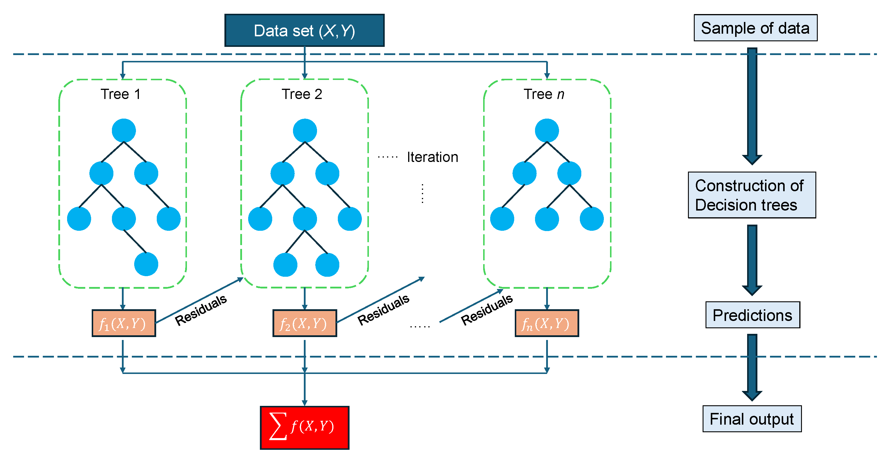
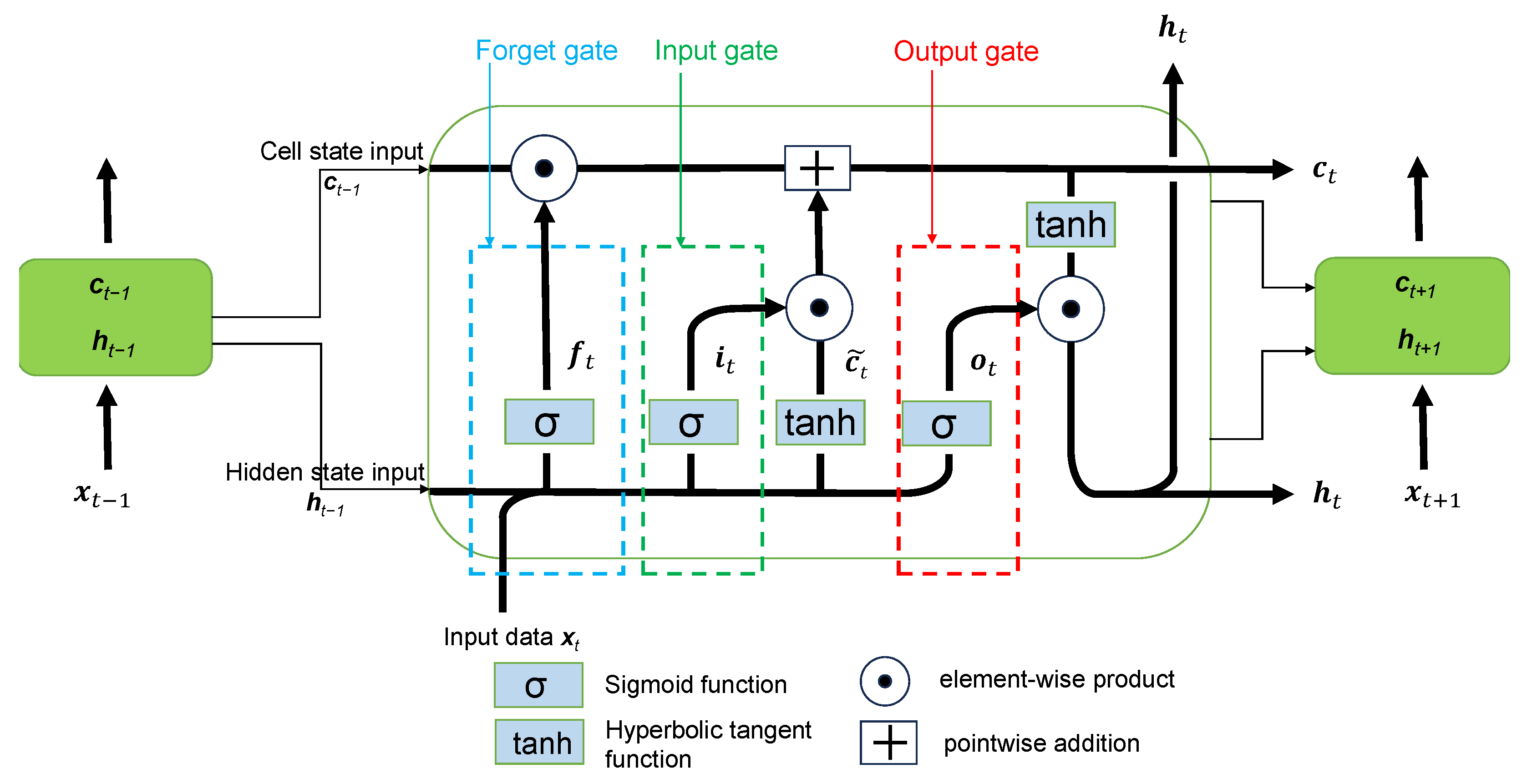


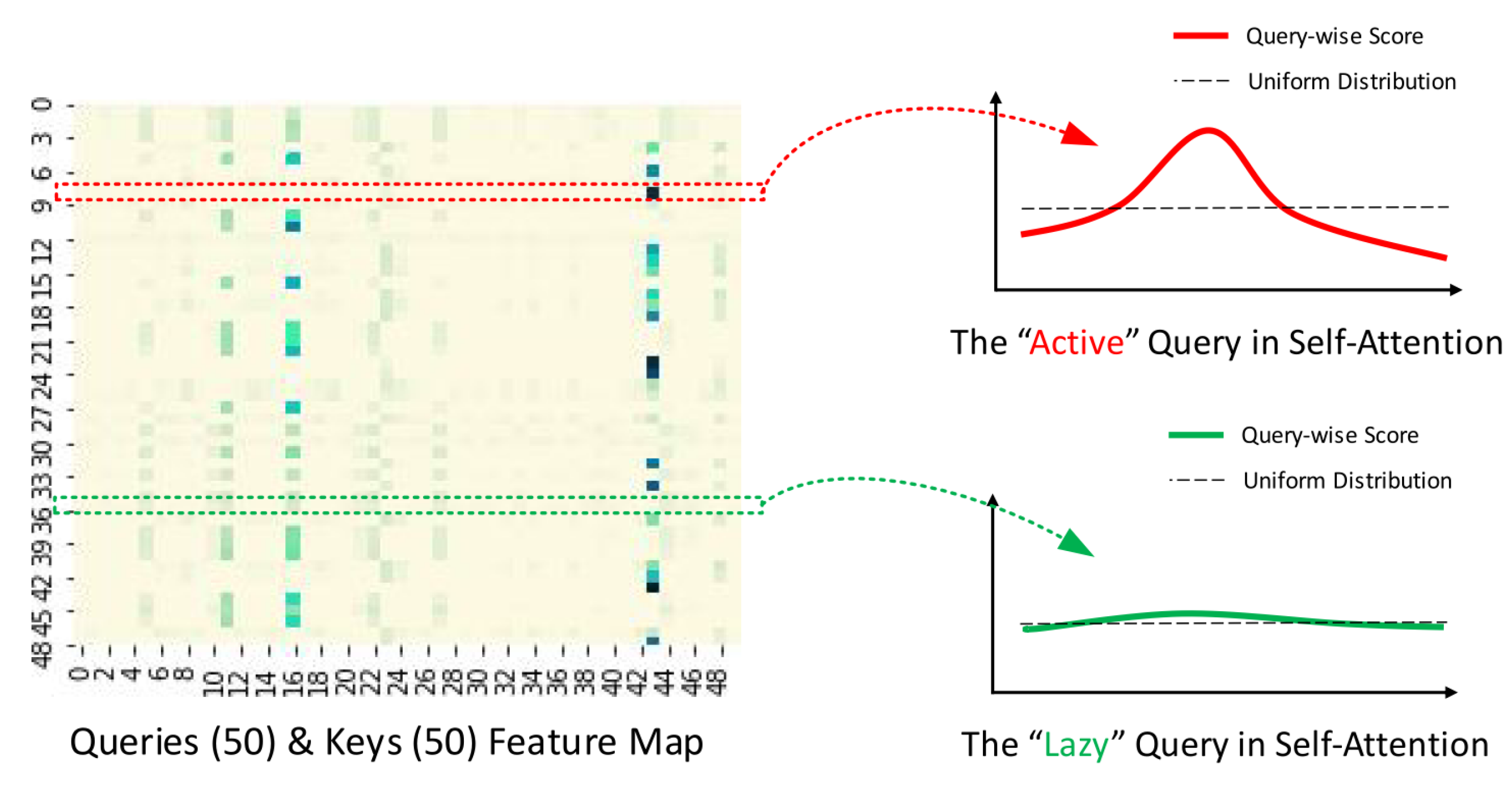
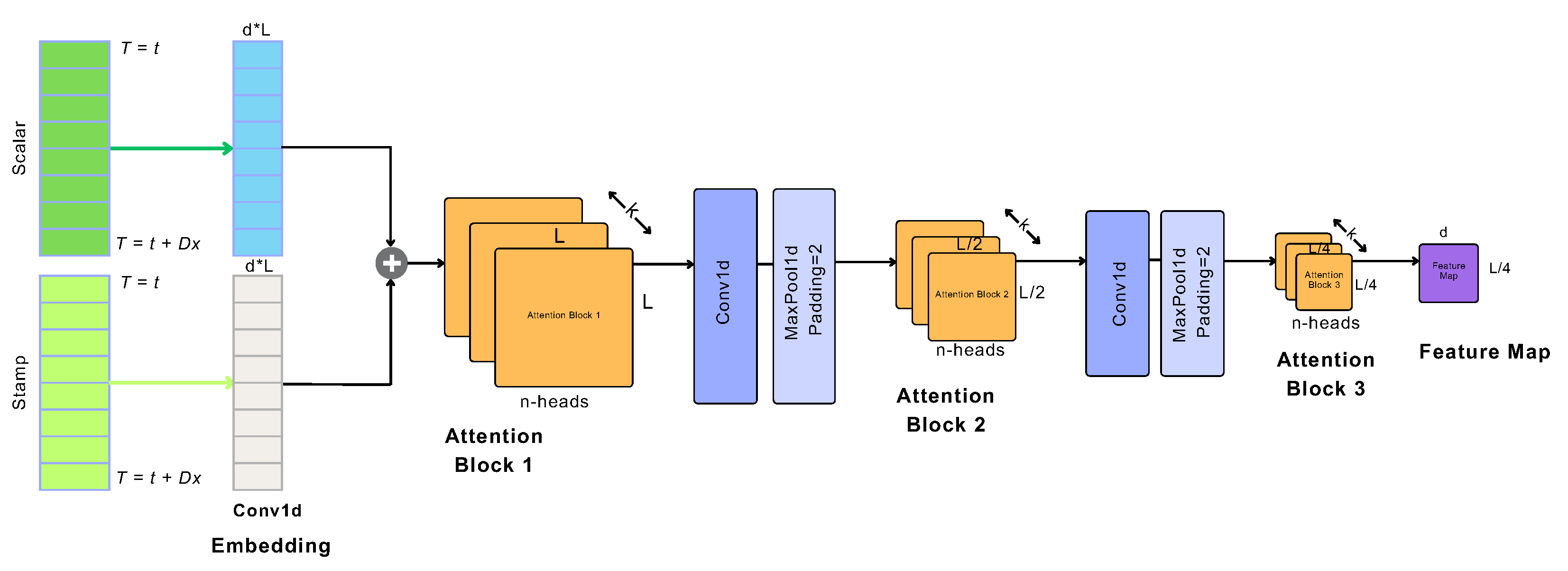
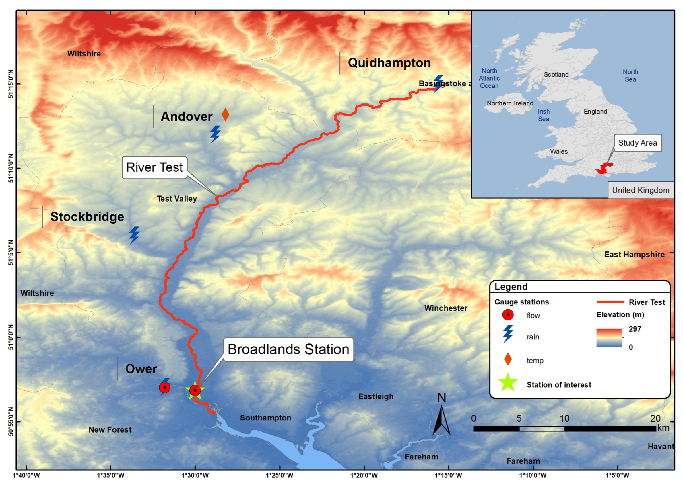
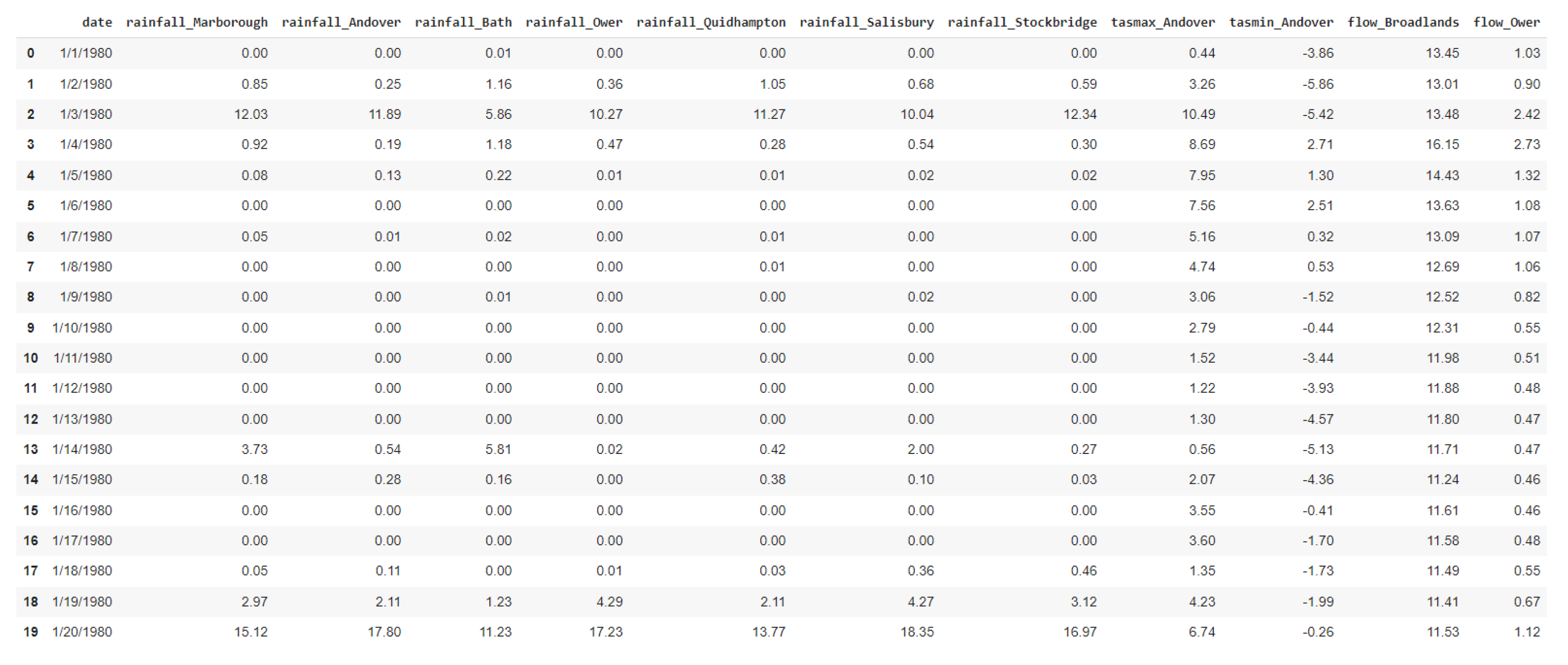
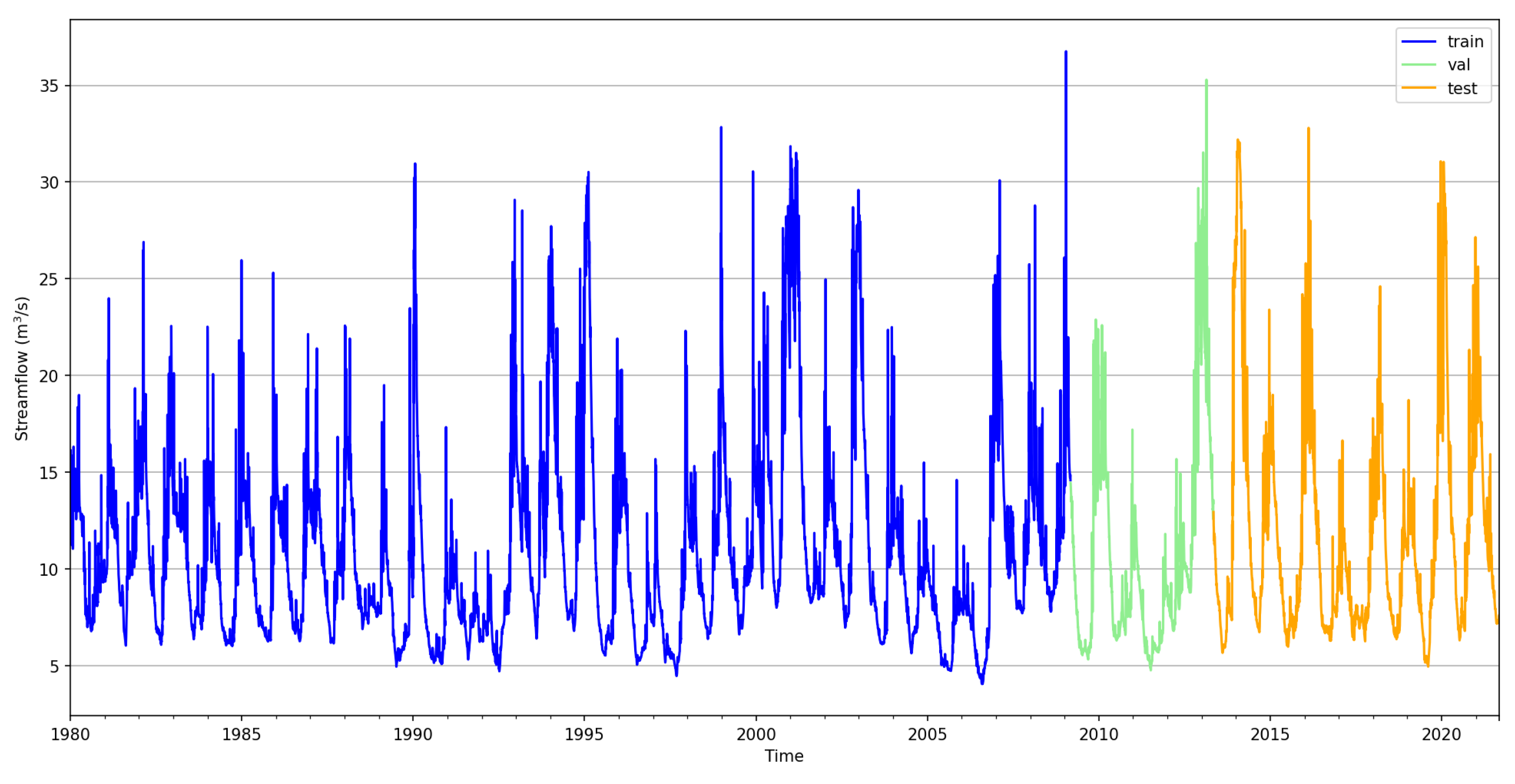
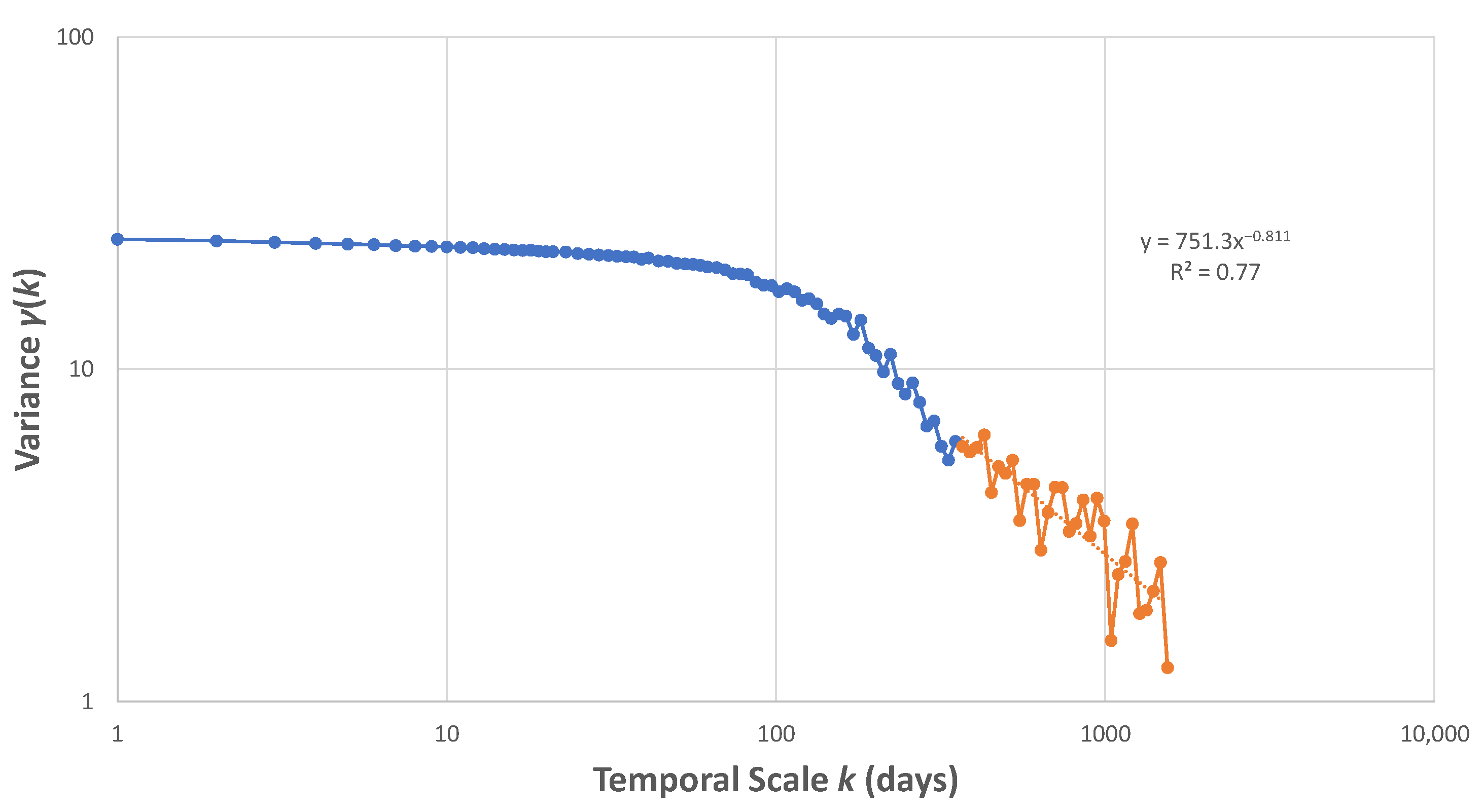
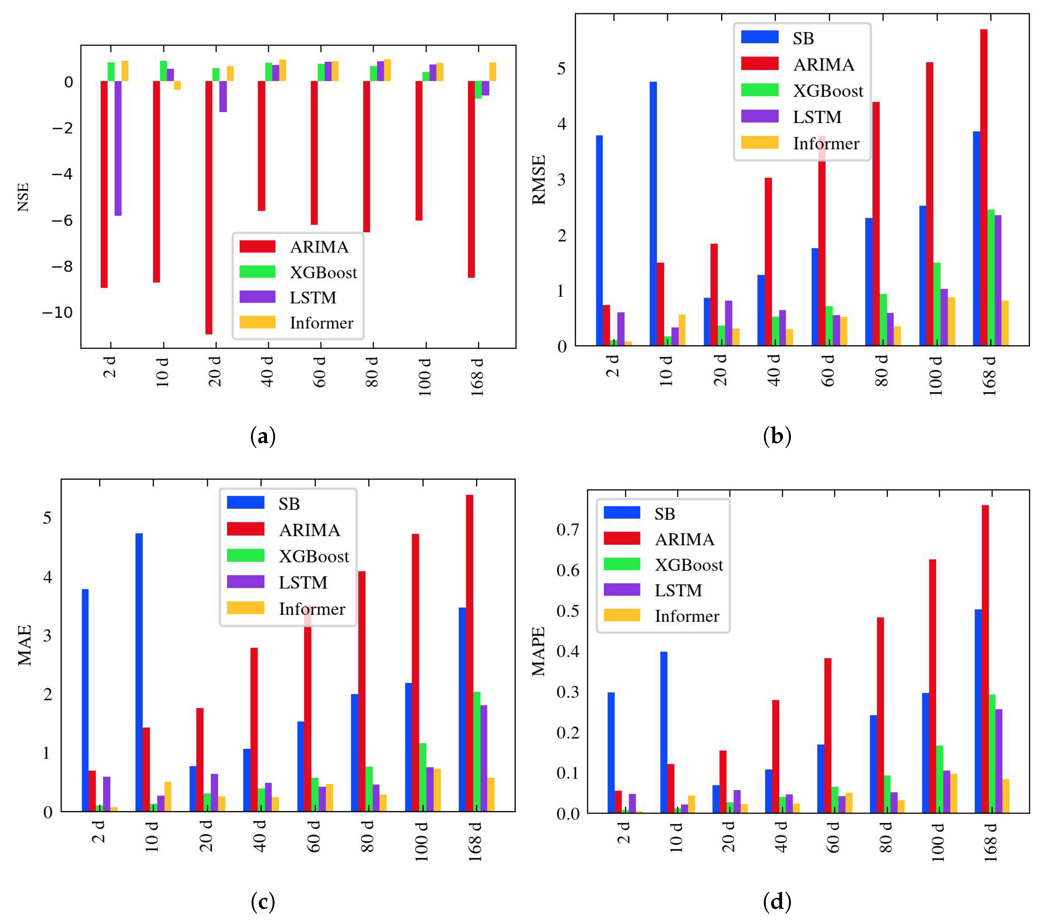
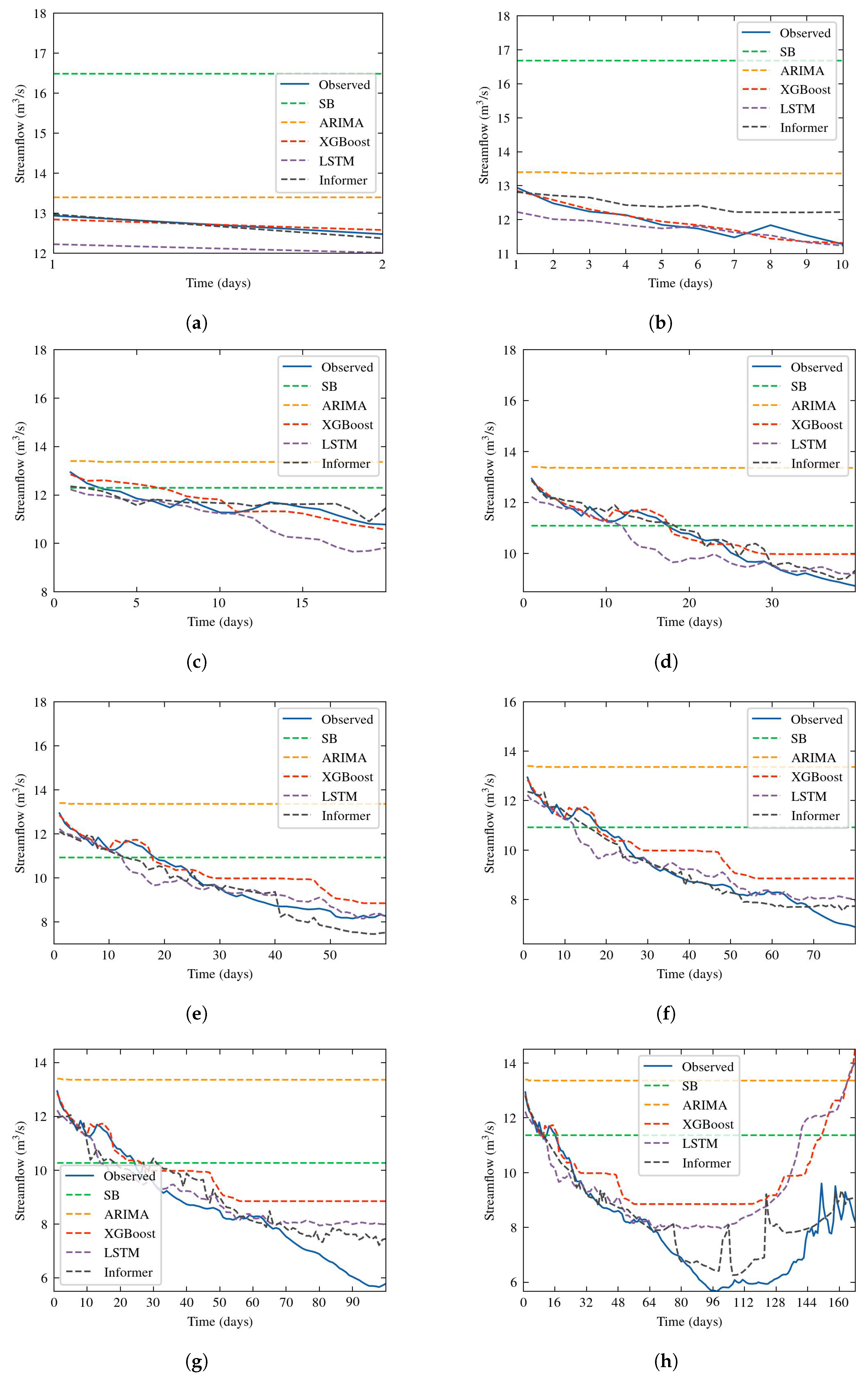
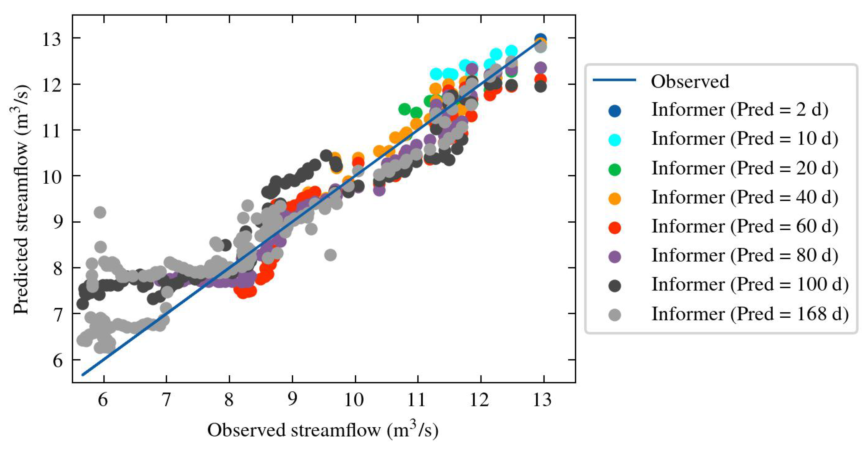
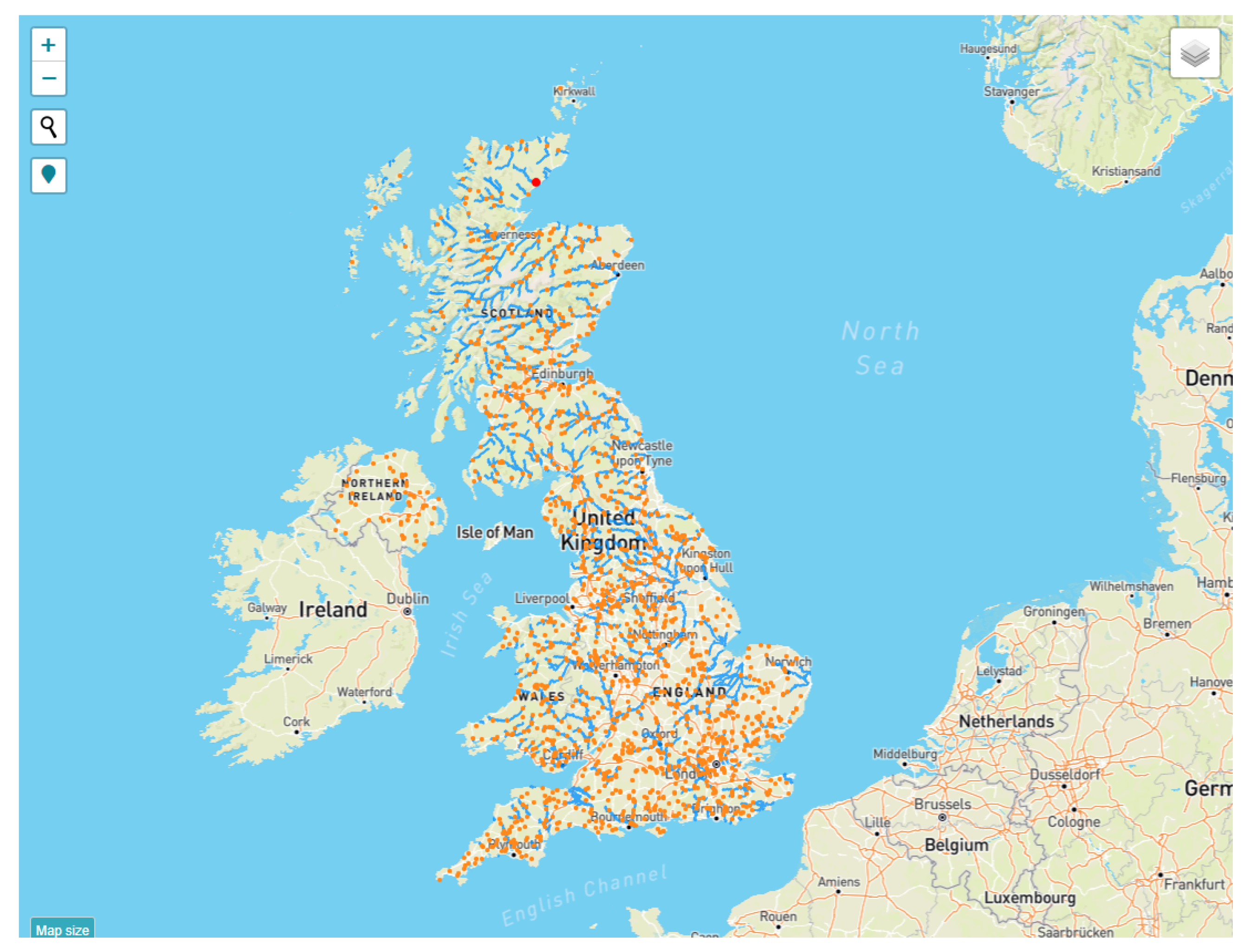
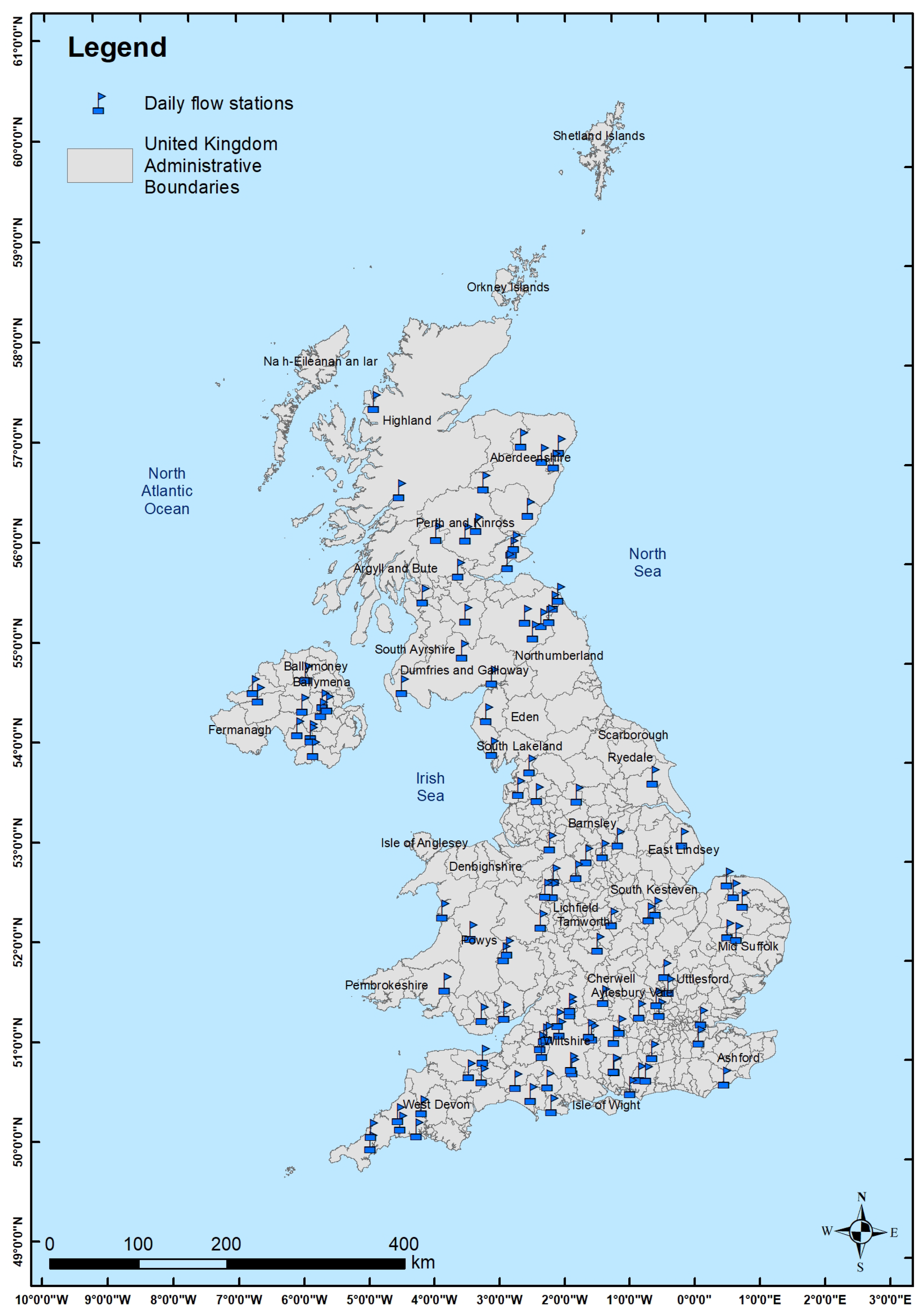
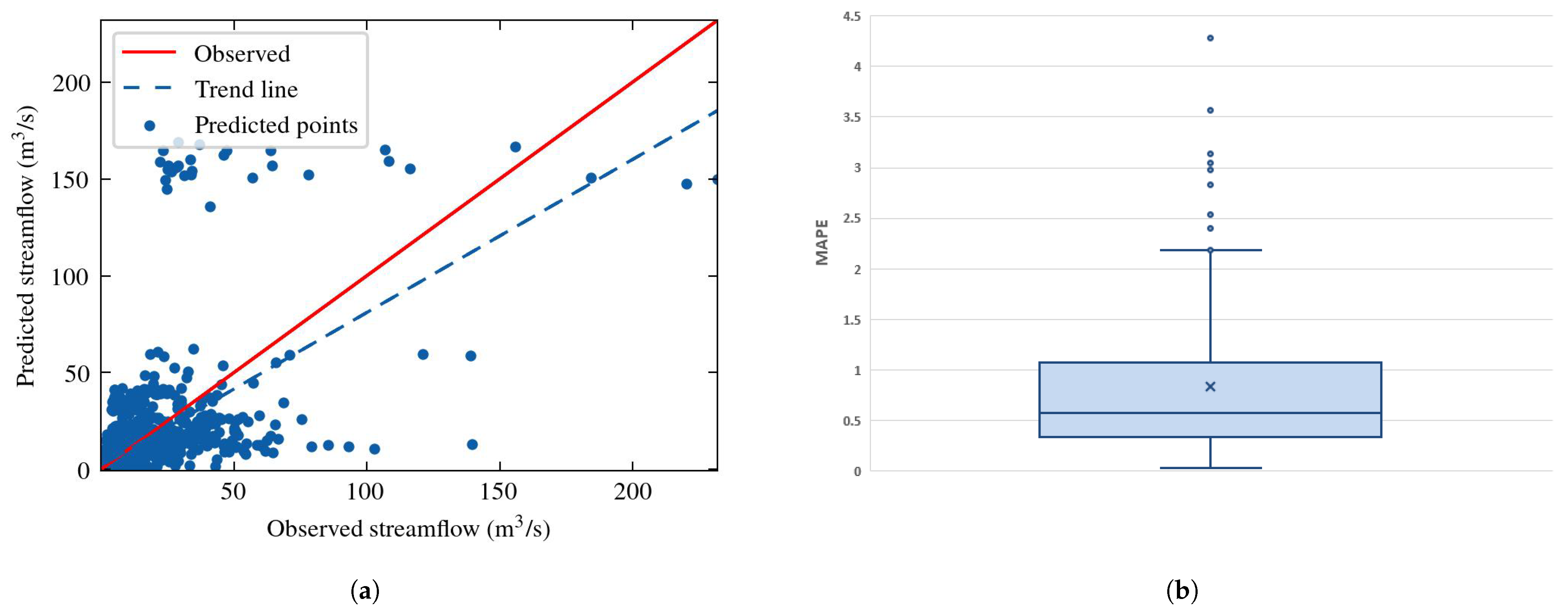
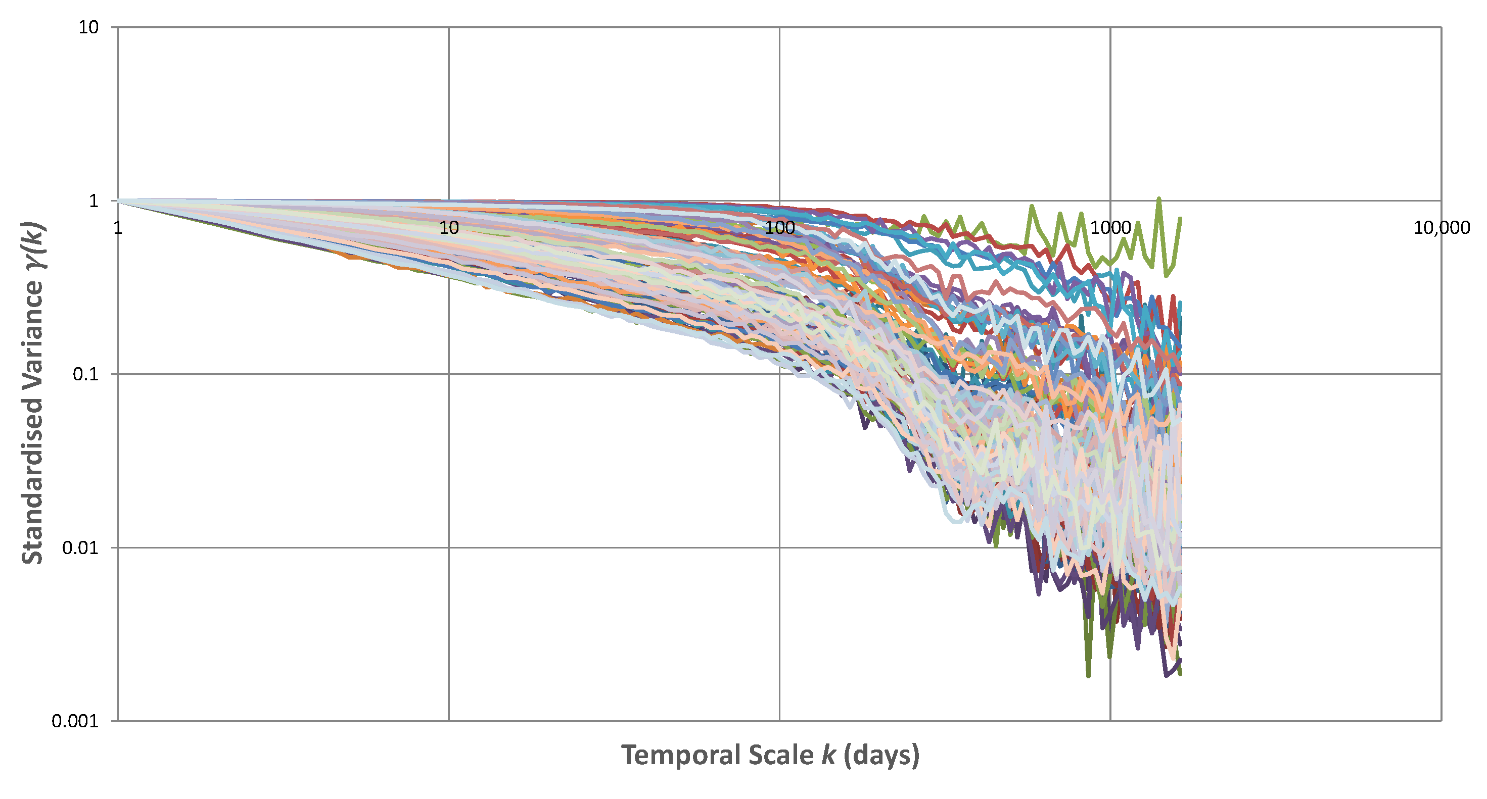

Disclaimer/Publisher’s Note: The statements, opinions and data contained in all publications are solely those of the individual author(s) and contributor(s) and not of MDPI and/or the editor(s). MDPI and/or the editor(s) disclaim responsibility for any injury to people or property resulting from any ideas, methods, instructions or products referred to in the content. |
© 2024 by the authors. Licensee MDPI, Basel, Switzerland. This article is an open access article distributed under the terms and conditions of the Creative Commons Attribution (CC BY) license (https://creativecommons.org/licenses/by/4.0/).