Abstract
Ongoing investments in irrigation technologies highlight the need to accurately estimate the longevity and magnitude of water savings at the watershed level to avoid the paradox of irrigation efficiency. This paradox arises when irrigation pumping exceeds crop water demand, leading to excess water that is not recovered by the watershed. Comprehensive water accounting from farm to watershed scales is challenging due to spatial variability and inadequate socio-hydrological data. We hypothesize that water savings are short term, as prior studies show rapid recharge responses to surface changes. Precise estimation of these time scales and water savings can aid water managers making decisions. In this study, we examined water savings at three 65-hectare sites in Nebraska with diverse soil textures, management practices, and groundwater depths. Surface geophysics effectively identified in-field variability in soil water content and water flux. A one-dimensional model showed an average 80% agreement with chloride mass balance estimates of deep drainage. Our findings indicate that groundwater response times are short and water savings are modest (1–3 years; 50–900 mm over 10 years) following a 120 mm/year reduction in pumping. However, sandy soils with shallow groundwater show minimal potential for water savings, suggesting limited effectiveness of irrigation efficiency programs in such regions.
1. Introduction
Within the western USA, policy makers overseeing irrigated systems are challenged with sustaining farm productivity and profitability while managing water resources [1]. It is not uncommon for water managers to develop programs to help producers sustain profitability following new water policy imposed on them [2]. Gaps of knowledge about watershed-scale responses to new programs limit the choices for water managers to select from [3]; uncertainty in program outcomes naturally steers the decision making. In cases where ecosystem water needs are in deficit, one choice for water managers is to encourage increased irrigation efficiency within a watershed with the hope that (1) this will lead to a reduction in pumping, and (2) the reduction in pumping will generate new ecosystem water. It is often assumed by decision makers that this newly generated ecosystem water will be equal in magnitude to a reduction in pumping—and will last in perpetuity. To the contrary of this assumption, a number of projects focusing on increasing irrigation efficiency have been met with marginal water returns [4], further kindling the need to understand the paradox between increasing irrigation efficiency and a lack of resulting water savings [5,6]. Within the umbrella of irrigation efficiency, irrigation scheduling technology solutions (e.g., digital soil mapping, remote sensing of crop stress, crop consultants, and soil moisture sensors) are receiving increased attention [7] from resource managers and corporate social responsibility (CSR) programs despite their unknown water saving potential. Therefore, a need exists to estimate the magnitude and longevity of water savings resulting from the adoption of irrigation scheduling technology at farm scale.
In areas where growing season totals of precipitation and irrigation are in excess of evapotranspiration (ET), a reduction in irrigation pumping may lead to an equal in magnitude reduction in groundwater recharge (enhanced by irrigation return flow) occurring below the irrigated land [8]. However, changes at the soil surface will take some amount of time to propagate through the vadose zone and reach the water table [9], defined here as the lag time. We hypothesize that the lag time will be relatively short given previous work relating changing surface conditions and responses in groundwater recharge [10,11]. However, it is over the lag time that changes occurring at the surface are not “felt” at the water table, and water is consequently “saved”. To better illustrate the concept, Figure 1 presents a hypothetical case study where there is a 100 mm yr−1 reduction in pumping, a corresponding 100 mm yr−1 reduction in recharge, and a 3-year lag time. Water savings is then calculated as the difference between the cumulative reduction in pumping and the sum of cumulative reduction in recharge and ET, which in this example is 300 mm. In an ideal case, reductions in pumping would be equal in magnitude to excess in water supply, thereby having no detrimental impact on crop yield. In locations that are under near optimal water supply or in water-stressed conditions, reductions in pumping may reduce ET (and potentially yield [12]), which would also contribute to water savings. We therefore define water savings as follows:
where WS is water savings (mm), Preduction is the reduction in pumping (mm), Rreduction is the reduction in groundwater recharge (mm), and ETreduction is the reduction in ET (mm).
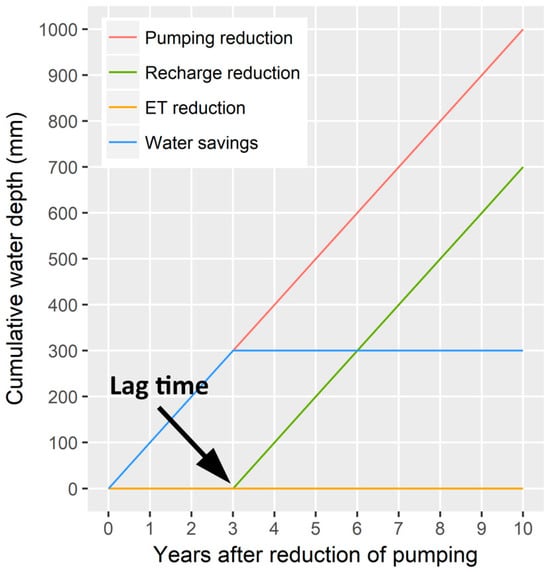
Figure 1.
Conceptual diagram of water savings and hypothetical case study. The lag time is defined by the amount of time that elapses following a reduction in pumping but before recharge rates begin to decrease. Lag times are a function of the depth to groundwater, soil water states and fluxes, and soil hydraulic parameters. Also note that the water savings are flat after 3 years, meaning no additional benefit, and that future management decisions can reduce water savings if pumping rates return to their initial rates or if field experiences prolonged periods of dry conditions.
As outlined in Figure 1, water savings are a function of the change in pumping, the resulting change in recharge and ET, and the corresponding time the vadose zone takes to respond. Given the transient nature of this problem, it is not easily resolved with simple mass balance approaches—particularly in environments with heterogeneous soil, land management, and varying depths to groundwater [10]. While outputs from physically based numerical modeling efforts often have high degrees of uncertainty [13], they can be a useful tool in exploring the impact of changing boundary conditions on water balance components, provided that model fluxes, states, and parameters can be reasonably constrained. With this in mind, localized study can be helpful to inform how key socio-hydrological factors vary within a given study area [14] and then potentially separate the relative individual weights of importance of those factors (e.g., soil, land management, and depth to groundwater) on water savings.
The focus of this work centers on a well-sampled study area located on the western fringe of the U.S. Corn Belt which is underlain by the High Plains Aquifer (HPA). Here, we have measured vadose zone parameters and fluxes, land management practices, and depths to groundwater across three field calibration sites (~65 ha each) in order to constrain realistic ranges of water savings in irrigated systems following technology adoption programs. This is an ideal place to study as (1) numerous agricultural producers in the area have been participating in a cost-share program facilitated by The Nature Conservancy to help producers reduce irrigation pumping through the use of on-farm technology and training, (2) the study site is located within a braided river valley and as such, significant soil variability is observed—we take advantage of this fact to explore differences in lag times due to different vadose zone hydraulic properties/thicknesses, and (3) approximately half the production fields in the study area are under water allocations, making this relevant work to inform future strategies to conserve water across the HPA and beyond.
As noted previously, water savings will in part be a function of the response of the vadose zone to reduced irrigation pumping. The response of the vadose zone will further be a function of soil moisture states, incoming and outgoing fluxes, soil hydraulic parameters, and thickness [10,15]. The significant spatial variability of soil within the study sites makes it challenging to locate a representative location to extract a soil core to represent the field average soil hydraulic properties, or more importantly, deep drainage rate. Previous work at the study sites by [16] found that time-repeat near-surface geophysical surveys processed through an empirical orthogonal function (EOF) statistical analysis were strong spatial predictors of shallow soil hydraulic parameters (0–30 cm). Viewing soil water fluxes through the lens of a process-based approach, we expect soil hydraulic properties to be strong drivers of water fluxes at depth. Therefore, and as a secondary hypothesis within this work, we suspect that time-repeat surface geophysical mapping would provide relative spatial patterns of water flux at depth. In order to test this hypothesis, we extracted three soil cores down to 6 m in each field at key locations informed by the geophysical mapping in order to bracket the range of deep drainage rates (defined as water flux below the root zone). Deep drainage rates were determined using a chloride mass balance (CMB) approach. Undisturbed cores were also analyzed in the laboratory to determine soil hydraulic parameters. Results from the CMB analysis were used to compare with outputs from a process-based numerical model (HYDRUS 1D, [17]) parameterized from the extracted soil cores. Following this validation exercise, we used the numerical model to explore the impact of reduced irrigation pumping on recharge (defined as flux at the top of the water table) as well as to calculate the magnitude and timing of ecosystem water savings.
The primary objectives of this work are to constrain water savings estimates that are the result of reduced irrigation pumping based on realistic ranges of vadose zone thicknesses and soil hydraulic parameters, reductions in irrigation pumping, and localized weather conditions. Additionally, we propose a method to bracket the variability of subfield water fluxes by smart sampling key locations within a field using the aid of a priori hydrogeophysical data. Using this approach, we are able to reduce time, cost, and effort associated with standard hydrogeological field techniques. Moreover, the hydrogeophysical maps provide more context and confidence that our deep drainage estimates constrain the range of subfield variability.
2. Materials and Methods
Table 1 provides a summary of analysis/methodology and its description in the study. The description specifies if the analysis was directly measured or modeled and how sensitive it is on the results if applicable. The following sections will describe in more detail each analysis/methodology.

Table 1.
Summary of analysis/method and description of how it is used in the study.
2.1. Description of Study Sites
The study area is located in western Nebraska within the river valley where the South Platte River enters the state (Figure 2) (N 41.007°, W 102.192°). The three study sites are each approximately 65 ha and 10 km apart primarily under irrigated maize production with overhead sprinkler irrigation. Soil texture in the area primarily falls within two USDA textural classes: sandy loam and loam. However, the landscape has been shaped by a braided river channel leading to significant soil variability on the subfield scale (<1 km2) ranging from coarse sands to heavy clays. The study area is semi-arid where annual crop (maize) evapotranspiration (ETc) is significantly higher than precipitation (P). The 10-year average annual P is 440 mm and ETc is 775 mm yr−1 (from 2008–2017) as referenced by the Nebraska Mesonet weather station (Big Springs 6SE) located within 10 km of the study sites. Depth to groundwater at each study site varies from 6 m to 16 m as measured by locally installed observation wells.
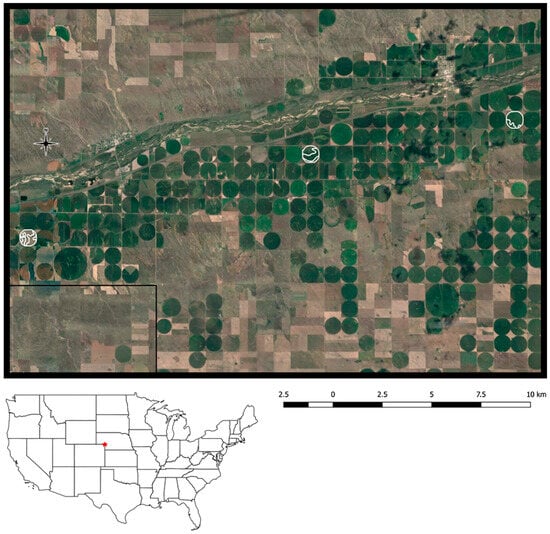
Figure 2.
Location of the three study sites near Brule, NE (red dot on USA). Each site is ~65 ha in area and primarily under irrigated maize production. White outlines are SSURGO soil boundaries. Field sites are S1, S3 and S4 from west to east.
2.2. Electromagnetic Induction Geophysical Mapping
Three hydrogeophysical surveys were collected at each of the three study sites using an all-terrain vehicle (ATV) as summarized by [16]. Surveys were carried out from the spring of 2016 to the spring of 2017 (exact dates can be seen in Table 2). Bulk electrical conductivity (ECa) maps were collected using a Dualem-21S electrical magnetic induction (EMI) sensor (DUALEM, Milton, Canada). Four simultaneous depths of ECa (mS m−1) can be measured with the sensor given the dual-geometry receivers at separations of 1 and 2.1 m from the transmitter (for this analysis only a depth of 3.2 m is considered). Measurements of ECa were obtained every second while being towed behind an ATV on a plastic sled at speeds of 8–15 km hr−1 with 8–10 row spacing (~7–9 m) taking ~75 min to conduct a survey. A Hemisphere GPS XF101 DGPS (Juniper Systems, Inc., Logan, UT, USA) unit recorded the location of each measurement. Following basic QA/QC of the ECa data [18], a spatial map with 5 by 5 m resolution was created using an inverse-distance weighting procedure with the ~5000 observations. We note here that temporal differences in ECa mapping stem from soil temperature, volumetric water content (VWC), and soil solute concentration [19]. VWC has been shown to account for approximately 50% of this variability [20]. Here, we take advantage of this fact to use changes in ECa as an indicator of relative change in both VWC states and subsurface water flux spatial patterns.
Table 2.
Geophysical survey dates with explained variance of 1st EOF.
Following the completion of the ECa surveys, an empirical orthogonal function (EOF) statistical analysis was carried out to highlight consistent relative patterns of ECa. Full details regarding the theory and motivation of this analysis can be found in the previous literature [16,21,22,23]; however, an overview is provided here. The EOF analysis is essentially a more well-known multivariate analysis: principal component analysis (PCA). EOF primarily differs from PCA in that instead of multiple covariates, the analysis considers the same covariate but at different points in time. The eigen decomposition, therefore, collapses the data into numerous orthogonal spatial patterns (EOF) that are invariant in time, and a set of time series referred to as expansion coefficients (ECs) that are invariant in space [22]. Using this approach, we can collapse the dataset into spatial patterns that each describe a given amount of variability throughout all geophysical surveys. By selecting the most important spatial pattern (assuming the variability explained is sufficiently high), we are able to highlight areas of the field that will tend to have a relatively low ECa value (implying consistently dry) and a relatively high ECa value (implying consistently wet).
2.3. Sampling Strategy and Soil Core Extraction
On 20 November 2017, three 80 mm diameter soil cores were extracted from each field to a depth of 6 m with a direct-push soil sampler with a MC7 attachment (Geoprobe, Salina, KS, USA). The cores were collected in four successive 1.5 m plastic liners. The location of each core extracted was determined by visual inspection of the 1st EOF ECa maps such that the numerical scale of each EOF ECa map was sampled in the high, low, and mid values. We emphasize here that this sampling strategy will not lead to an area-average estimate of soil texture, VWC, or soil water fluxes given the low number of sampled locations per field. Instead, we argue that it will bracket the range of soil texture and VWC—which we hypothesize will bracket soil water fluxes given our knowledge of process-based soil physics. This sampling strategy was selected in order to take advantage of soil texture variability to maximize our ability to quantify water savings over a range of soil textures. Following extraction, cores were immediately cut to 30 cm, capped with edges wrapped with electrical tape, and stored in coolers until placement in cold storage in the laboratory at 4 °C.
2.4. Laboratory Analysis
In order to determine Cl− concentration from extracted soil cores for later analysis in the CMB method, samples were first prepared following standard laboratory methods [24] briefly outlined here. Each 30 cm soil core was cut in half and sampled in the middle of the core, leading to 30 cm sampling intervals. Gravimetric water content was measured by weighing samples on a precision balance before and after drying in an oven at 105 °C for 24 h. Anion (Cl− and NO3−) concentrations were determined by first extracting pore water following the elutriation method of adding deionized water and shaking for 4 hrs. After shaking, the samples were spun in a centrifuge for 30 min to settle suspended particles. Diluted pore water was then filtered by pushing through a 1 µm filter. Filtered water samples were run through an ion chromatography system (Dionex, Waltham, MA, USA) and diluted anion concentrations (Cl− and NO3−) were determined. Because deionized water was added to samples as part of the elutriation process, pore water prior to dilution was back-calculated to determine in situ concentration. This back-calculation was carried out using a simple dilution equation:
where M1 is in situ pore water concentration (prior to laboratory dilution) (mg L−1), V1 is the volume of pore water in the soil sample (mL), M2 is measured concentration of diluted pore water (mg L−1), and V2 is the sum of added deionized water used in the analysis and V1 (mL).
2.5. Soil Hydraulic Property Measurement
In addition to the chemical and moisture sampling described in the previous section, each extracted core (6 m) was subsampled (6–8 times) following major changes in either lithology and/or gravimetric water content. The undisturbed soil cores were collected by pounding a 5 cm diameter (100 cm3) stainless steel cylinder into the corresponding segmented 30 cm long core, discarding the plastic extraction liner, and then removing the steel cylinder. Water retention data along with unsaturated hydraulic conductivity data were determined using a benchtop evaporative HYPROP (METER, Pullman, WA, USA). Additionally, a WP4C (METER, Pullman, WA, USA) was used to supplement HYPROP data with higher soil tension values. A KSAT device was used to measure hydraulic conductivity on the same core (METER, Pullman, WA, USA). This combination of devices allows for a wide sampling range of soil tension (pF ~ 1–4.2, where pF is the log10 of the absolute value of soil tension in units of cm) and corresponding VWC. Bulk density values were determined by (1) drying in an oven at 105 °C for 24 h and weighed on a precision balance to determine dry soil mass, and then (2) dividing the mass of soil by the corresponding volume (100 cm3). Following this, saturated water contents, , were calculated using the following equation:
where is soil dry bulk density (determined from above; g cm−3) and is mineral grain density, assumed here as 2.65 g cm−3. Water retention functions were then determined using the van Genuchten–Mualem model [25,26] as defined by
where (cm−1) is the inverse of air entry pressure, n (-) reflects the pore size distribution of a soil with m = 1 – 1/n, and l (dimensionless) is a parameter representing pore space tortuosity and connectivity, assumed to be equal to 0.5 here. Unsaturated hydraulic conductivity is then fit following
where is VWC (cm3 cm−3); (cm3 cm−3) and (cm3 cm−3) are residual and saturated VWC, respectively; h (cm) is pressure head; K (cm day−1) and Ksat (cm day−1) are unsaturated and saturated hydraulic conductivity, respectively; and Se is saturation degree (dimensionless) calculated as
2.6. Chloride Mass Balance
Chloride is often used as an environmental tracer within semiarid environments for many deep drainage and recharge estimation studies [27,28,29] and also specifically in irrigated cropping systems [30,31,32]. It is an attractive tracer as it is naturally occurring in precipitation and irrigation water and is inexpensive to analyze. Chloride in infiltrated water moves through the subsurface in a conservative manner [27,33], and because of this, the age of moisture in the vadose zone can be bracketed by comparing cumulative mass inputs at the surface with cumulative Cl− masses at depth.
To determine Cl− mass inputs at the surface, both precipitation and irrigation depths along with corresponding Cl− concentrations must be determined. Annual wet deposition of Cl− was determined from interpolated National Atmospheric Deposition Program stations (http://nadp.slh.wisc.edu/NTN/annualmapsByYear.aspx accessed on 15 November 2017). Recent records of annual irrigation depths were available from the center pivot irrigation systems and supplemented with land owner knowledge where available. Cl− concentrations were determined from several measurements of pivot water over two growing seasons (see Table 2 for water depths and Cl− concentrations). Using Equation (7), individual contributions are added together to calculate annual Cl− mass input:
where I is the average irrigation application over the study period (mm yr−1), is the concentration of Cl− in irrigation water (mg L−1), P is the average precipitation over the study period (mm), and is the concentration of Cl− in rainwater (mg L−1). We note here that the above only holds if it can be assumed that infiltrated water is vertical, and that other sources/sinks of Cl− are negligible (e.g., runoff/run-on).
Next, cumulative Cl− mass at depth () from an extracted core can be determined following Equation (8):
where i begins at the surface sample, n is the number of subsamples in the core, indicates the length of the sample interval (mm), is the volumetric water content defined above, and is the chloride concentration in pore water (mg L−1) at that sample.
The time passed since infiltration for any point in the extracted core can then be determined by dividing the total Cl− mass in the core by the annual Cl− input.
Finally, the deep drainage rate (mm yr−1) is calculated from Equation (10):
where i begins at the base of the root zone, indicates the sample interval length (mm), and tSUBRZ is the difference in time elapsed since infiltration for water between the base of root zone and the base of the core (calculated from Equation (9) assessed at the base of the root zone and the base of the core).
2.7. Numerical Modeling
A physically based vadose zone model, HYDRUS-1D (H1D) [17], was used to simulate the response of recharge rates (defined as flux occurring at the top of the water table) to a change in irrigation practice for each extracted core at the three study sites. H1D approximates the 1D Richards equation which represents the vertical redistribution of water and is calculated as
where is VWC, t is time (day), z is the distance between two measurement nodes (cm), K(h) is the unsaturated hydraulic conductivity (cm day−1), h is the pressure head (cm), and S is a sink term describing evapotranspiration (day−1). The simulated soil profile was 6–16 m deep depending on depth to groundwater determined from a local observation well. A constant head lower boundary condition (equal to 1 cm) is set for the lower boundary condition representing the top of the water table. Crop ET (ETc) was calculated using the single crop coefficient (Kc) method outlined in [34] as follows:
where Kc is a function of growing degree day accumulation (GDD) and ETr is ET for a reference crop. Regional Kc data were determined from the Nebraska Mesonet Stations and daily GDD values were calculated from daily minimum and maximum temperatures following [35].
The H1D model requires crop-referenced ET (ETc) to be separated into potential evaporation (Ep) and potential transpiration (Tp). This is carried out using Beer’s law:
where Tp is the potential transpiration (cm day−1), Ep is the potential evaporation (cm day−1), k is the light extinction coefficient (specified as 0.55 [35]), and LAI (m2 m−2) is the leaf area index. We simulated an LAI time series using Hybrid Maize [35] for each year’s growing season in order to inform Equations (13) and (14). Additionally, we followed the same processes described in [35] in order to represent the shape and development of a maize root zone. These crop development changes and triggered irrigation decision making algorithms were assessed within a daily timestep—made possible by linking together a series of 1-day-long simulations (totaling 10 years) by passing 1-day-long model outputs as inputs for the next day (full details on this process are outlined in [36]). These modifications were necessary to better represent how irrigation decisions are made, as the current H1D code is unable to consider a dynamically growing root zone with a specified shape, as well as VWC-triggered irrigation that is informed by more than one depth. Within the modeling exercise, the change in irrigation practice is consistent with observed changes in irrigation in the study area, and we assume here that this serves as a reasonable change in behavior given the soil, weather, and cropping practices in the study area.
In this work, we initialize each simulation by first running a 10-year-long simulation to remove any impact of an initial condition on model states or fluxes. Following this spin-up period, two simulations are then carried out that are identical save for irrigation practice: one that represents pumping in excess of crop water demand following a simplified checkbook approach (excess is approximately 120 mm yr−1) and is similar to historical long-term pumping rates in the study area (referred to henceforth as precipitation delayed, PD, and used in the spin-up period), and one that represents near-perfect management that tracks VWC states and triggers after VWC is depleted to a critical level (referred to henceforth as H) (see [36] for full details on both irrigation scheduling routines and how they were implemented in the H1D model). We note that only one core site per field was used to decide when to trigger irrigation in the H case scenarios. The core selected for this purpose was the one nearest to where each land owner indicated they typically check for VWC conditions, or in the soil unit with the largest area in the field. This step was taken to ensure that each field had the same amount of irrigation applied to each of the 3 cores as uniform irrigation systems are used in each field in practice.
After each simulation pair for each core was completed (1 simulation set per core, 3 cores per field, 3 fields, 18 total simulations), the recharge rates were then compared to the observations. When the time series of recharge for each simulation sets diverge, changes at the surface have propagated down to the water table. This period of time then defines the lag time for that core.
3. Results
3.1. Electromagnetic Induction
Results from the time-repeat geophysical surveys are shown in Figure 3. The first EOF explained 96%, 91%, and 69% in S1, S3, and S4, respectively, of the spatial variability. In general, there is some reasonable consistency between the EOF patterns/shapes and the USDA NRCS SSURGO soil boundaries. However, there is significant variability within a SSURGO boundary. If subfield management is of interest to landowners, this underscores the need for better digital soil mapping.
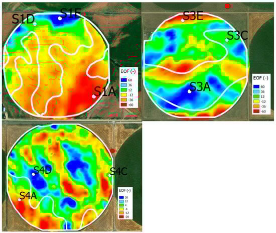
Figure 3.
Results of time-repeat ECa mapping from the Dualem 21S instrument (deep signal ~0–3.2 m) and the corresponding 1st EOF reprojected spatially for each of the three 65 ha study sites (see Table 1 for sample dates). Warm EOF colors indicate drier zones/coarser soil texture and cooler colors indicate wetter zones/finer soil texture compared to the field average. White lines are SSURGO soil boundaries. White dots are locations of core extraction (20 November 2017). Red dots are the location of the groundwater observation well (closest well to S1 was ~0.4 km away and not pictured here). Geophysical data layers can be found in Files SI1–SI3.
3.2. Laboratory Chemical Analysis
VWC and Cl− concentrations are summarized in Figure 4. Comparisons between soil cores indicate that VWC had a considerable range; 0.05–0.4 cm3cm−3. Cl− concentrations also varied considerably; <10–500 mg L−1. Both core-to-core variability and vertical variability within a core for values of VWC and Cl− followed major changes in soil textures (e.g., sandy soils tended to have lower VWC values). In the case of one core (S1A), vertical peaks in Cl− concentration had corresponding Cl− masses that were similar to annual mass input from irrigation water. Potentially, this could serve as an additional tracer method, but we note that applications here are limited as it was only observed in one of nine extracted soil cores. Concentrations of Cl− in the collected irrigation water samples were around 120 mg L−1 and varied less than ~10% from field to field and across the two growing seasons sampled (2016 and 2017; see Table 3). Compared to the wet deposition of Cl− from precipitation, the wet deposition from the irrigation source was three orders of magnitude higher (<0.2 g m−2 vs. ~50 g m−2).
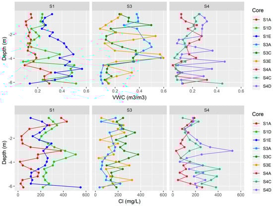
Figure 4.
Volumetric water content (VWC) and chloride (Cl−) concentration profiles of soil cores extracted from the three field sites. Line colors correspond to EOF values determined at the core location (e.g., warm colors correspond to negative EOF values, green colors correspond to near-zero EOF values, and cool colors correspond to positive EOF values; see Figure 3). Sawtooth patterns observed in VWC and Cl- profiles align with changes in soil textures. Data from this analysis can be found in SI4.
Table 3.
Irrigation application depths and Cl− concentration of samples collected from irrigation water (standard errors in parentheses). Depth to groundwater was determined from nearby observation wells.
3.3. Laboratory Soil Physics
Results of the fitted van Genuchten soil hydraulic parameters are summarized in Table 4. Bulk density ranged from 1.1 (g cm−3) to 1.9 (g cm−3) with an average of 1.5 (g cm−3) across the 59 samples measured. Residual water content ranged from 0 to 0.081 with numerous values set to zero in the fitting process. While not ideal and an artifact of the fitting process, samples with residual water content values of zero and large saturated hydraulic conductivity indicate the sample contained high amounts of sand and or gravel. The coarse aggregate in the samples was easily confirmed with visual inspection of the core. We note that previous work [37] has shown that n and α control behavior for unsaturated conditions so the poor fitting of some of these parameters has minimal impact on the results here. Each water retention function took approximately 4–5 days to complete the evaporative experiment.
Table 4.
Fitted van Genuchten water retention parameters. An * indicates the parameter was set to max in the fitting process.
3.4. Chloride Mass Balance Analysis
Deep drainage rates and the number of years represented within the core (determined by dividing total Cl− mass storage by annual Cl− mass input) can be found in Table 5. The mean deep drainage rate observed was 272 mm yr−1 with a median value of 215 mm yr−1. While the ranges of fluxes are considerable, we note here that they do not correspond to an area-average value due to the sampling strategy of likely targeting lower and upper boundaries of fluxes, along with the small number of samples per field (n = 3). Regardless, the average deep drainage rates compare well to a multi-year and multi-location lysimeter study carried out in the region where average deep drainage was determined to be 220 mm yr−1 [38] under similar cropping and irrigation systems. This observed rate is within 20% of our mean and within 2% of our median deep drainage rate. Additionally, ref. [39] reported total growing season ETa rates for 2016 to be 410 mm as estimated by a coupled remote sensing and soil measurement updated model for a field within 10 km of the study sites. These estimates combined with the findings of [36], describing historical long-term seasonal water supply of 700 mm across 50 fields in the area, would lead to a difference of 290 mm, which is within 6% of our mean and within 25% of our median deep drainage rate.
Table 5.
CMB analysis and numerical modeling results. Irrigation routine used for the numerical modeling in order to represent field-specific historical irrigation application is noted (soil moisture triggered (H)). S3A * had a heavy clay lens at ~3 m—flux calculated at this location may be unreliable as water flow may not have been 1D.
We note that one core, S3A, had a heavy clay lens at ~3 m as seen by visual inspection of the soil core. We speculate here that the existence of this clay lens may have led to non-1D flow of soil water which would impact the CMB calculation as this is an underlying assumption of the method. Given the relatively high flux calculated for this core and its contrasting heavy soil texture, we suspect that the CMB estimates are likely not reliable at this location.
3.5. Numerical Modeling
3.5.1. Validation of Numerical Model Water Balance Components
Across the nine simulated cores, modeled ET rates were on average 650 mm yr−1 (range of 500–750 mm yr−1) over the 10 years of simulation. This is consistent with average ET reported for the study area of 600–700 mm yr−1 as reported by [40]. While the average rates compare well, the range in our simulations is wider—likely due to differences in scale (i.e., point scale for a core vs. 1 km2) addressed by the two methods. Irrigation rates simulated across the three fields were within 10% of the historical averages for each field (Table 4).
Annual deep drainage rates determined by the numerical modeling are illustrated in Figure 5. Simulated deep drainage rates were low over the years 2012–2014, likely due to the extreme drought in 2012 (annual rainfall was 36% of the 10-year average). Given the year-to-year variability in simulated annual deep drainage rates, we report deep drainage numbers over the same time history of each individual core determined by the CMB analysis. For example, S1A had a 3-year time history (see Table 4). Therefore, in order to keep the time histories between the CMB analysis and numerical modeling consistent, we compare numerical modeling results for that core over 2015, 2016, and 2017 (the three most recent years). The average simulated deep drainage flux across all cores is 235 mm yr−1, which is within 84% of the average from the CMB analysis.
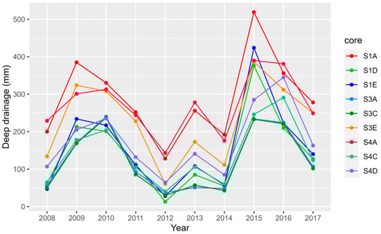
Figure 5.
Numerical modeling results of annual deep drainage; 2012 was an exceptionally dry year with 36% of average precipitation falling for that year. Bar colors correspond to EOF values determined at the core location (e.g., warm colors correspond to negative EOF values, green colors correspond to near-zero EOF values, and cool colors correspond to positive EOF values).
Figure 6 summarizes the VWC profiles over 6 m. In general, the shapes of simulated VWC profiles align with the major changes in lithology observed in the laboratory analysis. Some simulated cores show less variability than the corresponding measured core in vertical VWC profiles, likely due to only having 6–8 water retention functions measured per core. The root zone depth-integrated VWC has a strong correlation with the observed VWC from the core extraction (r2 = 0.81) (Figure 7). Here, we note that the EOF analysis was able to separate the depth-integrated VWC for both the measured root zone and modeled root zone values. This may be useful in future studies trying to connect spatial geophysical maps collected from the surface with root zone soil states and fluxes.
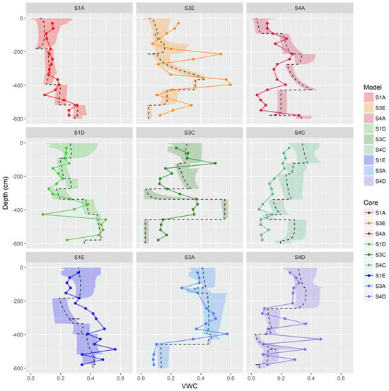
Figure 6.
Volumetric water content profiles from the core analysis overlain onto numerical modeling outputs. Bands are the minimum and maximum of ranges of the simulated VWC profiles and dashed lines are the corresponding simulated mean over the 10-year simulation period. Lines with circles are from the extracted volumetric analysis from core. Line and band colors correspond to the EOF values determined at the core location (e.g., warm colors correspond to negative EOF values, green colors correspond to near-zero EOF values, and cool colors correspond to positive EOF values).
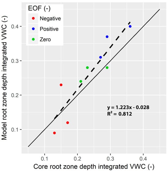
Figure 7.
Correlation between root zone depth integrated VWC for extracted cores and the corresponding simulated root zone depth-integrated VWC (10-year average). EOF values at each core location from the repeat geophysical analysis separate the relative ranges of depth integrated VWC for both the extracted cores and simulated soil profiles. Solid line is 1:1 and dashed line is best fit to data.
3.5.2. Lag Times and Water Savings
Figure 8 presents modeling results similar to the conceptual diagram and hypothetical case study presented in the introduction (Figure 1). A notable difference between the two figures is that Figure 8 shows that the reduction in pumping does not follow a straight line but instead one that is fairly episodic. Given that irrigation pumping rates do not occur consistently throughout a year, but instead over summer months, reductions to pumping will also occur discretely over each year.
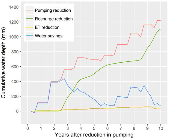
Figure 8.
Time series of model output determined at one core (S4C) from two paired simulations that vary only in irrigation scheduling routines. In this case, the lag time is approximately 2.5 years long (determined visually when recharge reductions begin to increase). Water savings are calculated as a cumulative reduction in pumping minus the sum of the cumulative reduction in recharge and ET.
As indicated by Figure 9, it can be seen that lag times are in the range of 1–3 years across all field sites and cores (noted by the first decrease in water savings for each time series). Typically, water savings are observed immediately following the reduction in pumping, and although increases and decreases from year to year are often observed, there is a general tendency to converge over time. The impact of seasonal weather on lag times is demonstrated in Figure 10. While we see a reasonable sensitivity to weather (lag times ranging within ±20% depending on the weather year), given the short lag times, we note that this uncertainty is unlikely to change conclusions about the longevity of water savings.
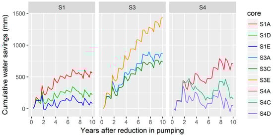
Figure 9.
Time series of simulated water savings calculated from the paired simulations for each core. Cores with coarser soil textures (S1A, S3E, and S4A) had the largest water savings as a result of a reduction in ET.
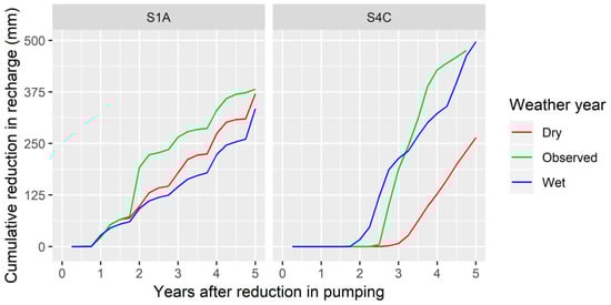
Figure 10.
Sensitivity analysis of weather year on estimated lag times and water savings. In both panels, simulations were carried out where a continuously repeated dry year is in red, a continuously repeated wet year is in blue, and the 10-year observed weather is in green. The 10th and 90th percentile weather years were selected for this analysis.
4. Discussion
4.1. Agronomic Reasonableness of Fluxes
Considerable differences are observed in VWC and deep drainage within each field site. In order to contextualize the reasonableness of the range of these fluxes, we compare yield differences between different core locations (only two fields had yield data available). In locations with low VWC and high deep drainage, there may be a higher potential for water stress leading to a lower yield. Indeed, this is the case, as can be seen in Table 6. Typically, we see similar patterns in the tabular data of yields and deep drainage. For example, core locations with low yields (relative to the other core locations) tend to have correspondingly high deep drainage rates and vice versa.
Table 6.
Yield data for two fields (S1 and S4) at location of extracted soil cores. Yield maps were unavailable for the S3 field. Yield data representing each core location were from an approximate 10 m2 area.
Additionally, we compare mass fluxes of NO3− within each core. If the observed water fluxes (determined from Cl− mass fluxes) are within reason, we should expect calculated NO3− mass fluxes to also be within reason—at least with respect to producer nitrogen fertilizer application rates and reasonable leaching rates. While we measured NO3− in the laboratory, we converted it to equivalent units of nitrogen (N) in order to compare it with other agricultural studies. Within the region, N leaching rates have been found to be near 50 kg ha−1 yr−1 for continuous maize rotations with corresponding deep drainage rates of 220 mm yr−1 as determined by multi-year and multi-location installed lysimeters [38]. Given our calculated water velocities from the CMB analysis, and the corresponding measured N masses, we find an average rate of 14 kg ha−1 yr−1 of N leaching. While perhaps on the low side given the sandy soil textures in the area, we show here that our deep drainage estimates fall within a reasonable rate relative to N losses. This serves as a sensible upper boundary check on our flux rates. For example, if deep drainage fluxes are considered too high, then we would expect corresponding N leaching rates to also be too high.
4.2. Applications to Subfield Soil Hydrology
Figure 7 shows the correlation between root zone depth-integrated VWC for extracted cores and the corresponding simulated root zone depth-integrated VWC. For both the simulated and observed depth-integrated VWC, the time-repeat geophysical analysis was able to separate relative differences from core to core across all three fields. This suggests that observed differences in VWC on the subfield scale are predictable with surface geophysics and resolvable through 1D numerical modeling. It currently remains unexplained why the geophysical analysis was able to indicate locations with high deep drainage as well as low deep drainage, but intermediate values of EOF did not correspond to intermediate values of deep drainage fluxes. We speculate that intermediate EOF zones may be the result of layering between two dominant soil types and that the layering effect may have a non-linear impact on flux. However, future work is needed to fully understand this effect. Regardless, being able to separate low and high deep drainage extends the findings of [16], who found that near-surface soil hydraulic parameters were key drivers of subfield soil moisture patterns (0–30 cm). Using geophysical layers as a covariate to inform soil hydraulic parameters as well as VWC states and fluxes may lead to better predictions of subfield yield variability driven by physical processes. Time-repeat geophysical mapping may also be a critical piece of additional information for improving estimates of the spatial variability of deep drainage across a field [41,42]. These data combined with input and output costs for production are useful in determining “profitability zones”. Future work could focus on using hydrogeophysics to refine the management of such zones.
4.3. Impact on Water Savings
Given the results in Section 3.5.2, we see modest returns of water savings (range of 50–900 mm over the 10-year simulated period). The range of water savings is largely explained by differences in ET rates following a reduction in pumping. In cases where pumping reductions are similar or less than excess pumping, deep drainage rates respond relatively quickly to the reduction in pumping, and thus a small amount of water is saved (50–200 mm) over a short period of time (1–3 years) and ET rates remain similar. This is contrasted with cases where the reduction in pumping is larger than the excess pumping. In this case, water savings are a combination of both the lag time and a reduction in ET, with ET reductions (and thus water savings) persisting indefinitely, and therefore, leading to larger water savings. This trade-off challenges water managers to choose between (1) reducing pumping to bring practices in line with crop water demand which may have short-lived outcomes but minimal impact on yield and farm profitability or (2) reduce pumping to put crops in/near a water-deficit state, leading to long-term water savings but at the cost of potentially reducing yield and decreasing farm profitability.
We note here that given the short lag times (1–3 years), a correspondingly short period of mismanagement or extreme drought may be able to reverse any water savings from good stewardship. For example, in Figure 8, water savings return to near zero following the extreme drought in 2012 (year 5 after reduction of pumping). In this situation, the drought occurred after recharge rates had equilibrated to the new reduction in pumping. However, the reduction in pumping for this year was near zero as both irrigation routines applied similar irrigation amounts due to a lack of rainfall leading to irrigation being triggered continuously (application only occurred every 3 days; consistent with center pivot systems). For this reason, water savings that are the result of a 1–3 year lag time may be challenging to maintain with changes in management, and especially when combined with the high variability of in-season convective rainfall patterns prevalent on the western edge of the U.S. Corn Belt.
Efficiency in center pivot irrigation can be in the range of 85–98% [43] due to evaporative losses of water (water evaporating before infiltrating the soil) depending on the sprinkler system utilized. Using the 120 mm yr−1 reduction in pumping used in this study, a corresponding reduction in evaporation of 3–19 mm yr−1 could be possible. However, we note here that this reduction in evaporation alone may not be large enough to justify a CSR program.
4.4. Optimizing Water Savings
Based on the various combinations of investigated factors (differences in soil texture, historical pumping rates, thickness of vadose zone), areas with sandy soil textures and shallow depths to groundwater lead to the lowest water savings. In order to avoid low returns of water savings, these fields should be minimized or avoided in future incentive programs. In an ideal case, selecting fields with thick vadose zones and loamy soils would likely return the maximum water savings. However, the finding that good management needs to be maintained as water savings can be easily reversed underscores the need for strong partnerships between producers and CSR programs. In addition, natural cycles of dry periods or prolonged drought due to climate change will further exacerbate low returns based on water savings CSR criteria.
4.5. Water Savings within Corporate Social Responsibility Programs
While the low end of the range of the reported water savings is relatively small in comparison to total pumping over 10 years (approximately 3–5%), if these savings are observed over numerous fields, the total volume saved will compare well to water saving efforts within other CSR programs. For example, if a CSR program were to work with 50 fields (~65 ha each), the total volume of water saved could potentially be 4.9 billion L (using a value of 150 mm saved per field) under similar soil, weather, and management conditions. Working with The Nature Conservancy, General Mills reported a similar water savings estimate following installation of drip irrigation in Irappuato, Mexico under horticultural crops in their 2012 Corporate Sustainability Report (2024 version available here https://globalresponsibility.generalmills.com/ accessed on 15 September 2024). These programs could potentially apply what we have learned within this work to target fields with loamy soil textures and thick vadose zones, if possible, thereby increasing the water savings of their programs.
4.6. Benefits Other than Water Savings
While not explored explicitly here, additional benefits of reductions in pumping should also be considered when assessing the total value of such programs. Numerous studies have focused on the benefits of proper irrigation scheduling and reductions in N losses. Locations to target for this type of water quality program may be opposite locations to avoid for a water quantity program (shallow depths to groundwater and sandy soils). Considering this, further work could try to optimize locations with hydrogeological factors that overlap in order to optimize both water quantity and quality benefits. At the very least, this type of work could inform the rank order of ideal locations to target in order to maximize project outcomes. Additionally, energy costs associated with the pumping of groundwater are not negligible in areas with moderate depths to groundwater. In contrast to water savings, both of these benefits (N and energy savings) will see returns year to year. However, all benefits must be compared to the potential for yield loss and the impacts to farm profitability.
4.7. Limitations of This Study
This study used direct observations of soil hydraulic properties, observed forcings, and realistic boundary conditions with a 1D Hydrus simulation. Results from the 1D Hydrus simulations largely agreed with the CMB of deep drainage in eight of the nine cores. As recorded by the well driller, the core at S3A contained clay material and was likely a clay lens at around 3 m, resulting in horizontal flow and invalidating the CMB analysis and 1D Hydrus simulations. The clay lens was not evident from the surface geophysical observations used for selecting site locations based on soil texture. This example highlights the challenge of using point data for estimating deep drainage with CMB and using 1D model simulations to make broader conclusions about water savings. Conversely, coupled land surface and 2D/3D groundwater simulations are now possible at regional and local scales [44,45]. However, anisotropic soil hydraulic properties and aquifer characterization at this scale remains challenging. In this region, the USGS has conducted detailed airborne electromagnetic induction surveys [46] to help estimate spatial aquifer properties, but this type of data remain sparse and aquifer properties remain largely unknown or a calibrated model parameter. Despite the simplicity and limitations, the 1D Hydrus model results illustrate the challenges and opportunities for quantifying water savings in these agro-ecosystems under different management and climatic effects.
5. Conclusions
A need exists in better evaluating the longevity and magnitude of water savings resulting from the adoption of irrigation scheduling technology at the farm scale. Nevertheless, it is becoming increasingly common for local, state, federal, and/or corporate social responsibility programs to cost share irrigation scheduling technology. However, work focused on the so-named paradox of irrigation efficiency has documented that technology is not a panacea and such programs can lead to increases in overall water use within the watershed. Thus, there remains a need for more realistic water savings calculations given the known physics occurring within the vadose zone. Here, we use a variety of field, laboratory, and 1D numerical modeling techniques to constrain the water savings estimates at three study sites in western Nebraska that overlay the High Plains Aquifer system and have been recent benefactors of a CSR program. Results show that while lag times are short and water savings are modest (1–3 years; 50–900 mm over 10 years), if applied over a nominal number of production fields, water saving programs can be competitive with other environmental CSR programs. In order to fully assess the value of this type of program, additional impacts such as reductions in nitrogen fertilizer leaching, energy savings, and yield impact must be considered within the scope of farm profitability. Our findings suggest that future CSR programs should target fields with thicker vadose zones and finer textured soils to maximize the water saving benefits. However, we caution if water managers aim to save substantial water from reduced pumping and allocate these water savings for other long-term uses, water savings may in fact be short lived as they are highly dependent on the continued responsible water stewardship of landowners and subject to natural and prolonged dry periods.
Supplementary Materials
The following supporting information is available online from: https://data.mendeley.com/datasets/xtsnhzr7ng/1, (accessed on 15 September 2024). Franz, Trenton (2024), “Data for: Groundwater Recharge Response To Reduced Irrigation Pumping”, Mendeley Data, V1, doi: 10.17632/xtsnhzr7ng.1, Files SI1–SI3, and data File SI4.
Author Contributions
Conceptualization, J.G. (Justin Gibson), T.E.F. and J.G. (John Gates); methodology, J.G. (Justin Gibson), T.E.F., T.G., D.H. and S.T.; formal analysis, J.G. (Justin Gibson) and T.E.F.; resources, J.G. (John Gates), C.M.U.N. and T.E.F.; writing—original draft preparation, J.G. (Justin Gibson) and T.E.F.; writing—review and editing, J.G. (John Gates), C.M.U.N., S.T., D.H. and T.G.; visualization, J.G. (Justin Gibson); supervision, T.E.F., J.G. (John Gates), C.M.U.N., D.H. and T.G.; project administration, T.E.F.; funding acquisition, T.E.F. and J.G. (John Gates). All authors have read and agreed to the published version of the manuscript.
Funding
This research is supported financially by the Robert B. Daugherty Water for Food Global Institute at the University of Nebraska, The Nature Conservancy, and the Research Council Grant-in-Aid from the Office of Research and Economic Development at the University of Nebraska–Lincoln. This research was funded by the USDA National Institute of Food and Agriculture, Hatch projects #1009760 and #1020768.
Data Availability Statement
The weather data presented in this study are available at http://www.hprcc.unl.edu/awdn/ (accessed on 15 November 2017) as part of the National Mesonet Program. The USDA SSURGO soil data presented in this study are available https://websoilsurvey.nrcs.usda.gov/app/ (accessed on 15 November 2017). The chloride mass balance, soil hydraulic parameter data, and geophysical surveys presented in the study are included in the article/Supplementary Materials (doi: 10.17632/xtsnhzr7ng.1), further inquiries can be directed to the corresponding author/s. Hydrus 1d is available for download at https://www.pc-progress.com/en/Default.aspx?hydrus-1d (accessed on 15 November 2017). The HYDRUS 1d input files and results supporting the conclusions of this article will be made available by the authors on request.
Acknowledgments
Access to field sites and datasets was provided by landowners, The Nature Conservancy, Western Nebraska Irrigation Project, and South Platte and Twin Platte Natural Resources District. A special thank you to the local landowners, Jacob Fritton, Catherine Finkenbiner, William Avery, and Matthew Russell for various assistance.
Conflicts of Interest
Justin Gibson was employed by the company Lindsay Corporation and John Gates was employed by the company CropX. The remaining authors declare that the research was conducted in the absence of any commercial or financial relationships that could be construed as a potential conflict of interest.
References
- Knox, J.W.; Kay, M.G.; Weatherhead, E.K. Water regulation, crop production, and agricultural water management—Understanding farmer perspectives on irrigation efficiency. Agric. Water Manag. 2012, 108, 3–8. [Google Scholar] [CrossRef]
- Environmental Defense Fund. The Future of Groundwater in California; Environmental Defense Fund: New York, NY, USA, 2018. [Google Scholar]
- Hess, T.M.; Knox, J.W. Water savings in irrigated agriculture: A framework for assessing technology and management options to reduce water losses. Outlook Agric. 2013, 42, 85–91. [Google Scholar] [CrossRef]
- Lauer, S.; Sanderson, M.R.; Manning, D.T.; Suter, J.F.; Hrozencik, R.A.; Guerrero, B.; Golden, B. Values and groundwater management in the Ogallala Aquifer region. J. Soil Water Conserv. 2018, 73, 593–600. [Google Scholar] [CrossRef]
- Grafton, R.Q.; Williams, J.; Perry, C.J.; Molle, F.; Ringler, C.; Steduto, P.; Udall, B.; Wheeler, S.A.; Wang, Y.; Garrick, D.; et al. The paradox of irrigation efficiency. Science 2018, 361, 748–750. [Google Scholar] [CrossRef]
- Ward, F.A.; Pulido-Velazquez, M. Water conservation in irrigation can increase water use. Proc. Natl. Acad. Sci. USA 2008, 105, 18215–18220. [Google Scholar] [CrossRef]
- Zhang, J.; Guan, K.; Peng, B.; Jiang, C.; Zhou, W.; Yang, Y.; Pan, M.; Franz, T.E.; Heeren, D.M.; Rudnick, D.R. Challenges and opportunities in precision irrigation decision-support systems for center pivots. Environ. Res. Lett. 2021, 16, 53003. [Google Scholar] [CrossRef]
- Perry, C. Efficient irrigation; inefficient communication; flawed recommendations. Irrig. Drain. 2007, 56, 367–378. [Google Scholar] [CrossRef]
- Rossman, N.R.; Zlotnik, V.A.; Rowe, C.M.; Szilagyi, J. Vadose zone lag time and potential 21st century climate change effects on spatially distributed groundwater recharge in the semi-arid Nebraska Sand Hills. J. Hydrol. 2014, 519, 656–669. [Google Scholar] [CrossRef]
- Grismer, M.E. Estimating agricultural deep drainage lag times to groundwater: Application to Antelope Valley, California, USA. Hydrol. Process. 2013, 27, 378–393. [Google Scholar] [CrossRef]
- Turkeltaub, T.; Kurtzman, D.; Bel, G.; Dahan, O. Examination of groundwater recharge with a calibrated/validated flow model of the deep vadose zone. J. Hydrol. 2015, 522, 618–627. [Google Scholar] [CrossRef]
- Passioura, J.B. Grain yield, harvest index, and water use of wheat. J. Aust. Inst. Agric. Sci. 1977, 43, 117–120. [Google Scholar]
- Xie, Y.; Cook, P.G.; Simmons, C.T.; Partington, D.; Crosbie, R.; Batelaan, O. Uncertainty of groundwater recharge estimated from a water and energy balance model. J. Hydrol. 2018, 561, 1081–1093. [Google Scholar] [CrossRef]
- Noel, P.H.; Cai, X.M. On the role of individuals in models of coupled human and natural systems: Lessons from a case study in the Republican River Basin. Environ. Model. Softw. 2017, 92, 1–16. [Google Scholar] [CrossRef]
- Rasmussen, T.C.; Baldwin, R.H.; Dowd, J.F.; Williams, A.G. Tracer vs. Pressure Wave Velocities through Unsaturated Saprolite. Soil Sci. Soc. Am. J. 2000, 64, 75. [Google Scholar] [CrossRef]
- Gibson, J.; Franz, T.E. Spatial prediction of near surface soil water retention functions using hydrogeophysics and empirical orthogonal functions. J. Hydrol. 2018, 561, 372–383. [Google Scholar] [CrossRef]
- Simunek, J.; van Genuchten, M.T.; Sejna, M. The HYDRUS Software Package for Simulating the Two- and Three-Dimensional Movement of Water, Heat, and Multiple Solutes in Variably-Saturated Media, Technical Manual; Version 1.0; PC-Progress: Prague, Czech Republic, 2006. [Google Scholar]
- Franz, T.E.; King, E.G.; Caylor, K.K.; Robinson, D.A. Coupling vegetation organization patterns to soil resource heterogeneity in a central Kenyan dryland using geophysical imagery. Water Resour. Res. 2011, 47, W07531. [Google Scholar] [CrossRef]
- Robinson, D.A.; Lebron, I.; Kocar, B.; Phan, K.; Sampson, M.; Crook, N.; Fendorf, S. Time-lapse geophysical imaging of soil moisture dynamics in tropical deltaic soils: An aid to interpreting hydrological and geochemical processes. Water Resour. Res. 2009, 45, W00d32. [Google Scholar] [CrossRef]
- Brevik, E.C.; Fenton, T.E.; Lazari, A. Soil electrical conductivity as a function of soil water content and implications for soil mapping. Precis. Agric. 2006, 7, 393–404. [Google Scholar] [CrossRef]
- Korres, W.; Koyama, C.N.; Fiener, P.; Schneider, K. Analysis of surface soil moisture patterns in agricultural landscapes using Empirical Orthogonal Functions. Hydrol. Earth Syst. Sci. 2010, 14, 751–764. [Google Scholar] [CrossRef]
- Perry, M.A.; Niemann, J.D. Analysis and estimation of soil moisture at the catchment scale using EOFs. J. Hydrol. 2007, 334, 388–404. [Google Scholar] [CrossRef]
- Finkenbiner, C.E.; Franz, T.E.; Gibson, J.; Heeren, D.M.; Luck, J. Integration of hydrogeophysical datasets and empirical orthogonal functions for improved irrigation water management. Precis. Agric. 2018, 20, 78–100. [Google Scholar] [CrossRef]
- Adane, Z.A.; Gates, J.B. Determining the impacts of experimental forest plantation on groundwater recharge in the Nebraska Sand Hills (USA) using chloride and sulfate. Hydrogeol. J. 2015, 23, 81–94. [Google Scholar] [CrossRef]
- van Genuchten, M.T. A Closed-form Equation for Predicting the Hydraulic Conductivity of Unsaturated Soils. Soil Sci. Soc. Am. J. 1980, 44, 892. [Google Scholar] [CrossRef]
- Mualem, Y. A new model for predicting the hydraulic conductivity of unsaturated porous media. Water Resour. Res. 1976, 12, 513–522. [Google Scholar] [CrossRef]
- Allison, G.B.; Hughes, M.W. The use of natural tracers as indicators of soil-water movement in a temperate semi-arid region. J. Hydrol. 1983, 60, 157–173. [Google Scholar] [CrossRef]
- Scanlon, B.R.; Reedy, R.C.; Stonestrom, D.A.; Prudic, D.E.; Dennehy, K.F. Impact of land use and land cover change on groundwater recharge and quality in the southwestern US. Glob. Chang. Biol. 2005, 11, 1577–1593. [Google Scholar] [CrossRef]
- Gates, J.B.; Edmunds, W.M.; Ma, J.; Scanlon, B.R. Estimating groundwater recharge in a cold desert environment in northern China using chloride. Hydrogeol. J. 2008, 16, 893–910. [Google Scholar] [CrossRef]
- Katz, B.S.; Stotler, R.L.; Hirmas, D.; Ludvigson, G.; Smith, J.J.; Whittemore, D.O. Geochemical Recharge Estimation and the Effects of a Declining Water Table. Vadose Zone J. 2016, 15, vzj2016. [Google Scholar] [CrossRef]
- Liao, L.; Green, C.T.; Bekins, B.A.; Böhlke, J.K. Factors controlling nitrate fluxes in groundwater in agricultural areas. Water Resour. Res. 2012, 48, 1–18. [Google Scholar] [CrossRef]
- Lin, D.; Jin, M.; Liang, X.; Zhan, H. Estimating groundwater recharge beneath irrigated farmland using environmental tracers fluoride, chloride and sulfate. Hydrogeol. J. 2013, 21, 1469–1480. [Google Scholar] [CrossRef]
- Scanlon, B.R.; Goldsmith, R.S. Field study of spatial variability in unsaturated flow beneath and adjacent to playas. Water Resour. Res. 1997, 33, 2239–2252. [Google Scholar] [CrossRef]
- Allen, R.G.; Pereira, L.S.; Raes, D.; Smith, M.; Nations, F.; United AO of the Crop Evapotranspiration. Guidelines for Computing Crop Water Requirements; FAO Irrigation and Drainage Paper 56; Food and Agriculture Organization of the United Nations: Rome, Italy, 1998. [Google Scholar]
- Yang, H.S.; Dobermann, A.; Lindquist, J.L.; Walters, D.T.; Arkebauer, T.J.; Cassman, K.G. Hybrid-maize—A maize simulation model that combines two crop modeling approaches. Field Crops Res. 2004, 87, 131–154. [Google Scholar] [CrossRef]
- Gibson, J.; Franz, T.E.; Wang, T.; Gates, J.; Grassini, P.; Yang, H.; Eisenhauer, D.E. A case study of field-scale maize irrigation patterns in Western Nebraska: Implications to water managers and recommendations for hyper-resolution land surface modelling. Hydrol. Earth Syst. Sci. 2017, 21, 1051–1062. [Google Scholar] [CrossRef]
- Wang, T.; Franz, T.E.; Zlotnik, V.A. Controls of soil hydraulic characteristics on modeling groundwater recharge under different climatic conditions. J. Hydrol. 2015, 521, 470–481. [Google Scholar] [CrossRef]
- Klocke, N.L.; Watts, D.G.; Schneekloth, J.P.; Davison, D.R.; Todd, R.W.; Parkhurst, A.M. Nitrate leaching in irrigated corn and soybean in a semi-arid climate. Trans. ASABE (Am. Soc. Agric. Biol. Eng.) 1999, 42, 1621–1630. [Google Scholar] [CrossRef]
- Barker, J.B.; Heeren, D.M.; Neale, C.M.U.; Rudnick, D.R. Evaluation of variable rate irrigation using a remote-sensing-based model. Agric. Water Manag. 2018, 203, 63–74. [Google Scholar] [CrossRef]
- Szilagyi, J.; Jozsa, J. MODIS-aided statewide net groundwater-recharge estimation in nebraska. Groundwater 2013, 51, 735–744. [Google Scholar] [CrossRef]
- Woodforth, A.; Triantafilis, J.; Cupitt, J.; Malik, R.S.; Subasinghe, R.; Ahmed, M.F.; Huckel, A.I.; Geering, H. Mapping estimated deep drainage in the lower Namoi Valley using a chloride mass balance model and EM34 data. Geophysics 2012, 77, WB245–WB256. [Google Scholar] [CrossRef]
- Weaver, T.B.; Hulugalle, N.R.; Ghadiri, H. Estimating Drainage under Cotton with Chloride Mass Balance and an EM38. Commun. Soil Sci. Plant Anal. 2013, 44, 1700–1707. [Google Scholar] [CrossRef]
- Yonts, C.D.; Kranz, W.L.; Martin, D.L. Martin Water Loss from Above-Canopy and In-Canopy Sprinklers; NebGuide G1328; University of Nebraska-Lincoln: Lincoln, NE, USA, 2007. [Google Scholar]
- Felfelani, F.; Lawrence, D.M.; Pokhrel, Y. Representing Intercell Lateral Groundwater Flow and Aquifer Pumping in the Community Land Model. Water Resour. Res. 2021, 57, e2020WR027531. [Google Scholar] [CrossRef]
- Yang, C.; Tijerina-Kreuzer, D.T.; Tran, H.V.; Condon, L.E.; Maxwell, R.M. A high-resolution, 3D groundwater-surface water simulation of the contiguous US: Advances in the integrated ParFlow CONUS 2.0 modeling platform. J. Hydrol. 2023, 626, 130294. [Google Scholar] [CrossRef]
- Center USGSCG and GS. Airborne Geophysical Surveys Conducted in Western Nebraska, 2010: Contractor Reports and Data; Open-File Report; U.S. Geological Survey: Reston, VA, USA, 2014. [CrossRef]


Disclaimer/Publisher’s Note: The statements, opinions and data contained in all publications are solely those of the individual author(s) and contributor(s) and not of MDPI and/or the editor(s). MDPI and/or the editor(s) disclaim responsibility for any injury to people or property resulting from any ideas, methods, instructions or products referred to in the content. |
© 2024 by the authors. Licensee MDPI, Basel, Switzerland. This article is an open access article distributed under the terms and conditions of the Creative Commons Attribution (CC BY) license (https://creativecommons.org/licenses/by/4.0/).