Abstract
This paper proposes an efficient productivity-aware optimization framework that utilizes hybrid machine learning with parallel global search to timely and appropriately adjust the critical control parameters (CCPs) of a cutter suction dredger (CSD) during construction. This optimization framework consists of three main parts. First, a hybrid Jaya–multilayer perceptron (MLP) algorithm was developed to rapidly construct a model that captures the interaction between construction parameters and slurry concentration. Next, the preliminary coarse results for the CCPs are determined through multi-parameter sensitivity analysis. Finally, the proposed resilient-zone parallel global search algorithm was employed to further optimize the CCPs, yielding more precise optimization results. To validate the proposed optimization framework and implement the in-situ service, it is applied to a real-world case study involving “Tianda” CSD construction. The results demonstrated that the average optimization duration is 6.7 s, which is shorter than the data acquisition interval of 8 s. Our approach improves the computational efficiency by 9.4 times compared with traditional optimization control methods. Additionally, there is a significant increase in the slurry concentration, with the maximum growth rate reaching 81.64%.
1. Introduction
As a crucial type of dredging equipment, the cutter suction dredger (CSD) is widely used in various dredging projects such as land reclamation, inland river dredging, and port construction [1]. Uncertainties in environmental factors such as underwater soil conditions and wind waves during construction necessitate dynamic adjustments of control parameters during excavation and construction processes [2]. Improper and untimely adjustments of CSD control parameters, often based on operators’ experience, can reduce excavation efficiency and delay the construction period [3]. Therefore, ensuring the correct and timely optimization of control parameters is crucial for improving the design efficiency of the CSD.
Several studies have been conducted to determine appropriate control parameters for the operation of the CSD. Wei et al. [4] conducted a combined experiment and simulation to investigate the slurry flow rate in the pipeline, aiming to reduce energy consumption and prevent blockage. To comprehend the flow characteristics of solid–liquid two-phase flow in the cutting system of a CSD, Zhang et al. [5] performed numerical simulations by employing the standard k-epsilon model and multiple reference frames to analyze the flow field within and around the cutting system. The findings provide a theoretical basis for optimizing operating parameters. Bai et al. [6] proposed a control model for the transverse movement process of dredgers based on CSD construction data using a linear regression algorithm, which was further applied in the design of subspace identification and prediction controller to ensure a stable output of slurry concentration (SC) and improve dredger operation efficiency. Shang et al. [7] introduced a construction optimization strategy based on real-time productivity regression analysis, using machine learning techniques to guide construction workers in adjusting certain parameters. The optimization of the CSD control parameters primarily focuses on two main aspects: (1) the integration of experimental verification and numerical simulation techniques [8,9,10,11] and (2) the utilization of data-driven machine learning methods, such as support vector regression (SVR), long short-term memory (LSTM), and multilayer perceptron (MLP) [12,13]. The former relies heavily on early pre-construction work, including high-precision experimental measurements, accurate numerical simulations, and sets of historical best cases. Numerical simulation methods typically involve the calculation of large matrices and require higher resolution spatial mesh subdivision and complex boundary conditions to simulate fluid flow states [14,15,16]. These factors lead to longer computation durations, making it difficult to provide timely guidance on control parameters during the construction process [17]. In contrast, data-driven methods can provide guidance based on objectives such as dredging yield and construction SC while reducing optimization duration [18,19,20,21]. Specifically, data-driven approaches extract hidden information from historical time series data to identify patterns and predict future trends [22,23,24]. However, most existing studies focus on model accuracy and the overall construction efficiency, with less emphasis on computation duration [25,26,27]. This results in a temporal lag that is not synchronized with the actual construction process [28]. Recently, approaches integrating artificial intelligence of things (AIoT) technology have emerged, which allow for real-time monitoring and dynamic optimization in response to evolving conditions during CSD operations. These systems leverage self-sensing concrete and advanced AI algorithms to continuously adjust dredging parameters, reducing the inherent temporal lag in traditional and data-driven methods. Thus, the further development of an effective, real-time parameter optimization framework is necessary to enable timely control strategies that synchronize with the CSD construction process.
In CSD construction management, setting and adjusting control parameters significantly impacts the overall efficiency of the construction process [17,29]. During the dredging process, the construction parameters exhibit the following characteristics: (1) Spatiality: This indicates that the monitoring parameters of CSD change along the construction path. (2) Multidimensionality: This implies that a multitude of data are monitored throughout the construction process due to the integration of multiple sensors in the supervisory control and data acquisition (SCADA) system installed in the CSD. (3) Timeliness: This signifies that the SCADA system continuously monitors and records all parameters during every stage of construction. (4) Cross-correlation: This denotes intricate relationships among the various monitoring parameters recorded during the CSD construction process [17,18,26]. Exploring the extensive and timely optimization of control parameters will lead to a more comprehensive understanding of CSD parameter control research [30]. These complex characteristics of monitoring data make analyzing mounts of monitoring data and establishing relationships between multidimensional parameters more challenging.
The cornerstone of achieving an efficient productivity-aware control parameter optimization framework of CSD is the utilization of efficient data-driven models to examine the intricate and nonlinear relationships between timeliness monitoring parameters [30,31]. The deployment of efficient and straightforward algorithms is important for the optimization of critical control parameters (CCPs) [32]. Machine learning algorithms has been extensively used to explore diverse construction parameters, establish implicit relationships between monitoring parameters, and provide guidance to improve construction efficiency [33,34,35,36]. Moreover, a number of methodologies have been proposed for the purpose of optimizing control parameters. Yao, Wang, Shang, and Zhang [19] introduced a nonlinear productivity optimization model based on the Lagrange algorithm, which provides an optimal value range for critical construction parameters. However, this method requires a significant number of input parameters, and the selection of these parameters greatly impacts the results, making it complex for construction personnel to implement. The complexity of parameter selection and the accuracy of the optimization results present significant obstacles to applicating this method directly in engineering projects. On the other hand, Wei et al. [37] suggested using a neural network model to create a virtual environment based on data from experienced CSD operators. They then used reinforcement learning models to develop optimal control strategies through interactions with this virtual environment. However, this approach requires several hours of data collection with experienced operators and suffers from limited learning samples, preventing reinforcement learning agents from effectively addressing uncertainties in actual soil changes during construction. Therefore, it is crucial to develop an optimization framework that can be efficiently applied during the construction. This optimization framework should have minimal computational duration, a simplified structure, and fewer parameter settings. Consequently, this study established a productivity-aware control parameter optimization framework for CCPs in CSD construction.
To address the aforementioned challenges, this paper presents an efficient productivity-aware control parameter optimization framework for CSD construction, leveraging machine learning with parallel global search, specifically designed for the dredging engineering industry. The primary contributions of this paper are as follows: 1. Taking into account the spatiality, multidimensionality, timeliness, and intercorrelation of monitoring parameters during CSD construction, a construction parameter–SC interaction model is developed through the data mining of the monitoring data. 2. A multi-parameter sensitivity analysis method is applied to obtain preliminary rough results for CCP optimization. 3. A resilient-zone parallel global search (RZPGS) algorithm-based optimal control strategy was developed to optimize CCPs, enabling timely and accurate parameter adjustments. 4. The proposed optimization framework preserves calculation accuracy while significantly reducing algorithm computation time, enhancing its potential for practical engineering applications.
The remainder of this paper is organized as follows: Section 2 outlines the construction process of CSD, details the optimization theory and methodology for CCPs, and describes the proposed efficient productivity-aware control parameter framework, providing further elaboration on the overall modeling flow and the methods employed in critical steps. Section 3 presents a case study on the construction monitoring of the “Tianda” CSD, which discusses the results and the effectiveness of the proposed framework. Finally, the conclusions and research perspectives are presented in Section 4.
2. Theoretical Foundations and Framework
2.1. Preliminaries
2.1.1. Dredging Construction of CSD
CSD is a type of vessel designed for the purpose of excavation activities in rivers, ports, bays, and similar environments. It is primarily composed of the reamer cutting system, SCADA system, transverse system, and slurry conveying system. Among these systems, the reamer cutting system is particularly important and requires timely control by technicians during construction, directly impacting the efficiency of the construction process [5]. Additionally, the SCADA system documents a multitude of construction data throughout the process, providing data feedback to workers and storing information in a database for subsequent research or other purposes.
The overall configuration of the CSD is illustrated on the left side of Figure 1. The cutter head, located at the front, is linked to the dredging pump through a suction pipe. The cutter head is capable of rotating along the axis of the suction pipe, which facilitates the fragmentation of soil or rock into smaller pieces. Once loosened, the material is efficiently extracted by a centrifugal dredging pump. The slurry intake inlet, situated beneath the cutterhead, is directly linked to the mud pump through a suction pipe. The vacuum created at this inlet effectively draws up loose soil particles. Subsequently, the pumped material is transported through pipelines to designated discharge areas. During the construction process, the CSD primarily relies on the transverse movement of its cutter head to accomplish dredging tasks. As depicted in on the right side of Figure 1, the hull rotates around a central steel pile in an arc trajectory during the dredging process. After completing the swing dig operation, the cutter head depth or steel pile position can be adjusted for the next excavation.
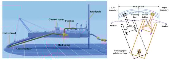
Figure 1.
Schematic of CSD structure and construction process: hull structure of CSD and schematic diagram of cutter traversing process [2].
Parameters that can be manually adjusted during construction are referred to as controllable parameters, while those that are significantly influenced by other factors and that cannot be directly manipulated are designated as uncontrollable parameters. Controllable parameters can be divided into two categories: real-time control parameters and preset parameters. Real-time control parameters are those adjustable parameters that operators can modify during the excavation process. Preset parameters are predetermined values established before each construction cycle, typically remaining unchanged during the excavation work. The classification of construction parameters is shown in Table 1.

Table 1.
The classification of construction parameters.
2.1.2. Theory of Control Parameter Optimization
This section provides a theoretical explanation for the rationale behind selecting transverse speed and cutter head velocity as the CCPs. In dredging projects, instantaneous production represents a crucial metric for evaluating the performance of a CSD and determining construction efficiency [38]. Equation (1) presents the calculation formula for the instantaneous production.
where W represents the instantaneous production, r is the radius of the slurry discharge pipeline, v represents the flow rate measured by the built-in detector in the pipeline, and p represents the SC. During dredging operations, the value of r remains constant, while v changes to a very limited extent. Consequently, p can be employed as an appropriate indicator for the evaluation of instantaneous yield. Furthermore, the volume of soil excavated by the cutter head primarily determines the SC during dredging operations. An increase in the SC can enhance productive efficiency to a certain extent. However, concentrations above a certain threshold may present a risk of pipeline blockage. Consequently, when maintaining an optimal concentration interval (where and represent the maximum and minimum values within this range, respectively), it is considered that the CSD is undergoing efficient construction.
The volume of material removed during excavation depends on three key factors: the longitudinal cutting thickness (excavation step length), the vertical cutting thickness (cutting depth), and the transverse speed. Therefore, the volume of material removed by the cutting head in a given time interval can be calculated using Equation (2).
where represents the volume of slurry entering the pipeline in a given time interval; denotes the cutter head excavation coefficient, typically ranging from 0.8 to 0.9 [39]; represents the volume of slurry excavation in a given time interval; refers to the longitudinal cutting thickness (excavation step length); signifies the vertical cutting thickness (cutting depth); and indicates the transverse speed of the CSD.
As demonstrated by Equations (1) and (2), several controllable parameters, including cutter head velocity, transverse speed, pump power, step length, and cutting depth, exert a significant influence on the instantaneous production [40]. When there is negligible alteration in soil quality at the construction site, pump power, excavation step length, and cutting depth are the preset parameters that remain unchanged throughout a construction cycle [41]. This paper primarily addresses optimizing CCPs when soil quality is relatively stable. Consequently, the adjustment of pump power is not significant in this paper. In conclusion, within a single excavation cycle in CSD construction, transverse speed and cutter head velocity are CCPs that are closely linked to excavation efficiency. In addition, it should be noted that in this paper, after data processing, the slurry concentration is uniformly expressed as the mass concentration.
2.2. Proposed Optimization Framework
2.2.1. Overall Workflow
The proposed optimization framework aims to optimize the CCPs of CSD accurately and timely, thereby enhancing the efficiency of construction. The specific steps are as follows:
Step 1: Establish the construction parameters–SC interaction relationship model.
Substep 1.1 Data preprocessing. Given the high dimensionality, substantial volume, disparities, and fluctuations in the original construction parameters archived in the SCADA system, data preprocessing is imperative. The goal is to mitigate the impact of outliers and enhance the efficiency and accuracy of data analysis. In addition, for the convenience of calculation, the slurry concentration monitored by multiple sensors in the pipeline is uniformly converted into mass concentration.
Substep 1.2 Establish the construction parameters–SC interaction relationship model. The construction parameters–SC interaction relationship model is established on the basis of processed construction data and SC data. It predicts the SC corresponding to the optimized results of CCPs during subsequent optimization processes. Simultaneously, the model assesses whether distinct sets of construction parameters fall within the optimal range for the SC.
Step 2: Conduct a multi-parameter sensitivity analysis of the CCPs.
Substep 2.1 Selection of CCP combination. The transverse speed () and cutter head velocity () are identified and selected as CCPs, with their combination specified as (, ).
Substep 2.2 Orthogonal experimental design. For the selected CCP combination (, ), the variables of transverse speed () and cutter head velocity () are considered as two dimensions. The gradient and number of gradients are defined in each dimension, after which an orthogonal combinations experiment is conducted.
Substep 2.3 Determination of optimal parameters adjustment combination. The construction parameters–SC interaction relationship model is employed to anticipate the SC for each combination of CCPs. Subsequently, a comparison is conducted between the predicted SC outcomes corresponding to each CCP combination in order to determine the optimal configuration. The evaluation process yields preliminary outcomes, which provide a foundational comprehension of the optimal results.
Step 3: Establish the optimization framework for the CCPs of CSD.
Substep 3.1 Optimization variables and objective. In the optimization of CCPs, and are considered as the optimization variables, with as the optimization objective. According to Equation (1), the value of can be calculated by , reaching its maximum when is at its peak. Furthermore, is a function of numerous monitoring parameters, as described in Section 3.2. Additionally, the CSD construction parameter control range is imposed as a constraint, facilitating the optimization of CCPs using Equation (3).
where represents the relationship between the construction parameters and the SC interaction, as described in Section 3.2.
Substep 3.2 Obtain optimization result. The RZPGS algorithm is utilized to solve the model in Equation (3) and identify the optimal CCPs. The efficient productivity-aware control parameters optimization framework is illustrated in Figure 2.
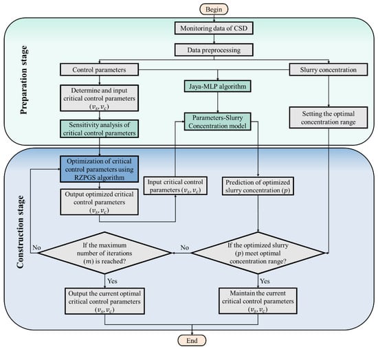
Figure 2.
The proposed efficient productivity-aware control parameters optimization framework.
2.2.2. Construction Parameters–SC Interaction Relationship Model
During the construction process, the monitored parameters and the SC undergo real-time, synchronous changes. To further investigate the impact of adjusting CCPs ( and ) on the SC, an implicit model was initially established to correlate various construction parameters, including 255 dimensions of monitored data from the SCADA system, with SC, as shown in Equation (4).
where represents the relationship between the construction parameters and the SC interaction. The MLP model is selected for the construction parameters–SC model due to its inherent convenience and flexibility.
The MLP is a methodology that has gained considerable traction in the field of implicit modelling. In accordance with the universal approximation theorem, the MLP functions as a fully connected feedforward neural network, incorporating multiple hidden layers [42,43]. Deploying a sufficient number of neurons within these hidden layers allows for precise approximations of spatially defined continuous input–output functions with notable accuracy [44]. Thus, selecting an MLP model offers a pragmatic approach to delineating the relationship between the construction parameters and SC. An MLP architecture encompasses an input layer, one or more hidden layers, and an output layer, all intricately interconnected, as depicted in Figure 3. Beyond the input node, each node embodies a neuron featuring a nonlinear activation function. Neurons in each hidden layer perform transformative weighting operations, converting values from the preceding layer into output values [45].
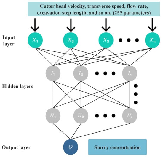
Figure 3.
The structural diagram of the MLP model (note: “X1, X2, X3, …, Xn” represents the neurons in the input layer, “I1, I2, I3, …, Is” and “H1, H2, H3, …, Ht” represent the neurons of the hidden layer, and “O” represents the neurons in the output layer).
However, the monitored parameters exhibit a high degree of multidimensionality and involve a substantial volume of data. Using the MLP algorithm for the construction of the training set may result in local optima, impeding the achievement of global optima. Additionally, determining the optimal connection weights and bias values for MLP represents a significant challenge. This challenge can be effectively addressed by employing a suitable heuristic algorithm for training. The Jaya algorithm, a heuristic algorithm, operates on the principle of continuous improvement. Individuals in the population move towards better individuals while distancing themselves from worse ones based on their respective distances from an excellent individual. Consequently, this approach facilitates the identification of optimal connection weights and biases [46].
Compared to other intelligent algorithms, the Jaya algorithm is distinguished by its simplicity, as it does not require the setting of complicated parameters. For specific problems, only two basic parameters (population size and iteration number) need to be set, eliminating the need for additional calculations to optimize objective functions through parameter adjustments [47,48]. Due to its simplicity and ease of implementation, the Jaya algorithm is well suited for addressing a wide range of optimization problems. In this study, the Jaya–MLP model was employed to establish an implicit relationship between the construction parameters and SC. Figure 4 illustrates the flowchart of the Jaya–MLP model. In this context, represents the value of the th variable for the th candidate solution after iteration , while and denote the best and worst solutions after iteration , respectively. and are random numbers between 0 and 1. The values of and indicate the tendency of candidate solutions toward the optimal solution and the extent to which the candidate solution avoids the worst solution, respectively. Consequently, the quality of the updated candidate solutions is continuously improved. This iterative process enhances the efficiency and precision in obtaining optimal connection weights and bias values for the MLP model, fostering convergence. Therefore, this approach ensures the refinement of the MLP model for superior performance.
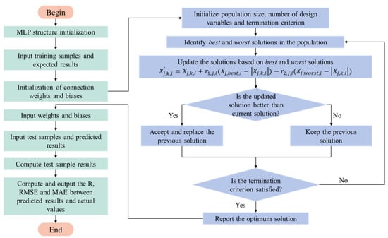
Figure 4.
The flowchart of the Jaya–MLP model.
2.2.3. Multi-Parameter Sensitivity Analysis of CCPs
During the construction process, fluctuations in the dynamic state of the CCPs and SC. Additionally, potential interactions among various construction parameters, especially those associated with the reamer cutting system, become evident [27]. Alterations in and depend on the current value of the other parameter, signifying a strong interdependence between these two variables. Therefore, conducting a multi-parameter sensitivity analysis is imperative for understanding the impact of fluctuations in CCPs on the SC. The methodology for the sensitivity analysis of control parameters is outlined as follows:
Step 1: The CCPs in Section 2.2 are selected as transverse speed () and cutter head velocity (), which form a combination of CCPs, denoted as (, ).
Step 2: Analyze the distribution characteristics of and . Subsequently, in accordance with the characteristics of the parameter distribution characteristics, establish and as the gradients for parameter changes, with and denoting the corresponding number of gradients for conducting orthogonal experiments. The arrangement of the orthogonal experiments is detailed in Table 2.
Table 2.
The orthogonal table for CCP combinations (, ).
Step 3: Using the construction parameters–SC interaction relationship model, predict the SC for each CCP combination within the orthogonal set. Compare the forecasted SC values and identify the CCP set with the highest anticipated SC as the optimal parameter adjustment configuration. This methodology establishes preliminary coarse results.
2.2.4. RZPGS-Based Optimal Control Strategy
After completing the multi-parameter sensitivity analysis, the further refined optimization of the CCPs is imperative to provide precise guidance for construction. The conventional grid search algorithm, a direct approach to hyperparameter optimization, systematically explores all possible CCP combinations within the parameter space to accurately identify the optimal solution. The grid search algorithm has been widely used in parameter tuning and optimization due to its simplicity and ease of implementation in real-time scenarios [45]. However, due to its exhaustive nature, this method is computationally expensive and time-consuming, posing a challenge in meeting the temporal constraints for the timely feedback of optimization results in construction projects [49].
Advances in computer hardware technology have enabled the use of multi-core processors for the CCPs of CSD, providing a hardware foundation for parallel computing. Recognizing that parallel computing enhances the computational efficiency and considering the ease of operation of the grid search algorithm, this paper proposes an enhanced RZPGS algorithm based on the conventional approach. By adjusting the computational step sizes and using different cores for simultaneous computations across multiple dimensions, this method significantly improves the computational efficiency. Figure 5 illustrates the basic principle of the RZPGS algorithm, involving the following fundamental steps:
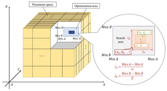
Figure 5.
Illustration of the RZPGS algorithm.
Step 1: Define the hyperparameter space and generate a grid. Identify the dimensions of the hyperparameter space to be explored, along with the respective ranges for each dimension (, , , ). Subsequently, create a grid on the hyperparameter space, where each point on the grid corresponds to a unique set of values for different hyperparameters.
Step 2: Initialize the partitioning scheme for the search area. Within the search space, define the initial search point , ). Determine the region partitioning parameters based on the characteristics of each dimension. Initialize the search step size matrix , and construct the step parameter structure matrix .
Step 3: Establish the parameter points evaluation method. Utilizing the previously proposed construction parameters–SC interaction relationship model as the assessment model for parameter points, conduct an evaluation and comparison of the identified parameter points.
Step 4: Execute the RZPGS algorithm. Cross all hyperparameter combination points within the search area, including (, (, (, ). Validate the optimization results for each parameter combination using the construction parameters–SC interaction relationship model.
Step 5: Identify the precise optimal parameters combination and output the optimal solution.
The initial search point , ) serves as the anchor for constructing a rectangular grid for exploration within the RZPGS algorithm. The introduction of region partitioning parameters enhances the search efficiency and facilitates the identification of the optimal grid point. The selection of the search step size in each dimension is contingent upon the search step size matrix , and it requires adjustment based on the respective dimension range. The search step size in each dimension can be expressed as detailed in Equation (5).
where represents a step size matrix of order , represents the search step sizes along the respective dimensions , and represent the maximum and minimum values, respectively, along the dimensions . Additionally, are defined as the region partitioning parameters, with values being positive integers (). The introduction of the region partitioning parameters enables the integration of engineering expertise, thereby facilitating the adjustment of search step sizes in different dimensions according to practical considerations. For instance, a smaller step size coefficient can be assigned to dimensions with minimal impact on the results, while the search step size is proportionally increased. Conversely, an increase in the step size coefficient in dimensions with a lesser impact will effectively reduce the search step size. The simultaneous evaluation of multiple parameters, when coupled with parallel computing, significantly accelerates the search process.
Once the optimization process has been configured, predefine cycles of searches. In the th search, generate random numbers between 0 and 1 to establish the initial generation of the step parameter structure matrix with dimensions , as exemplified in Equation (6).
where are all random numbers between 0 and 1. The new parameter points are thus acquired. The matrix representing the new parameter points in each dimension is displayed in Equation (7).
The new calculation method for parameter point coordinates can be derived as Equation (8) by substituting Equations (5) and (6) into Equation (7).
The newly obtained parameter point is input into the model to derive the optimization result , which is then compared with the optimization result corresponding to the parameter point . If does not surpass , it becomes necessary to regenerate a new set of step parameters to construct matrix and iterate through the aforementioned steps. Furthermore, if no improvement is observed for consecutive instances, adjustments are made to the step matrix in order to expand the search range. On the other hand, if outperforms , further assessment is required to determine whether this parameter point represents a local optimal solution. Subsequently, the step size matrix for each dimension must be configured individually in order to compute the new parameter point . At this junction, an optimization model is employed to derive the optimization result , which is then evaluated in terms of its superior over previous results. If is found to be superior, is considered to be a local optimal solution. Simultaneously, the extent to which fulfils the stipulated output criteria is evaluated. In the event that the aforementioned conditions are met, the parameters from each dimension of are output accordingly. However, in the event that no improvement is observed for consecutive instances or if the optimization result falls outside the output range criteria, adjustments are made to the region partitioning parameters, increasing the search step size and continuing the search until reaching an optimal outcome is reached or the cycle limit is reached.
The algorithmic process dynamically adjusted the search step for each dimension parameter during RZPGS, thus facilitating parallel calculations in each dimension. This methodology markedly enhances the efficacy of parameter optimization, while concomitantly guaranteeing the stability of the resulting optimization outputs. Moreover, this approach consistently explores each combination of parameters within the parameter space, thereby ensuring the stability of the outputted optimization results.
However, the CCPs investigated in this study are and , hence transforming the multi-dimensional RZPGS algorithm into a two-dimensional optimization issue. The region partitioning parameters and in the step size matrix can be assigned random positive integers ranging from 1 to 10 during encoding for computational convenience. At the initial stage of construction, the initial CCP combination () is input into the construction parameters–SC interaction relationship model for prediction. The model assesses whether the initial SC falls within the optimal concentration range. If it meets the criteria, the parameters are designated as the current optimal control parameters ( and ) and the SC is regarded as the current optimal concentration (). The output result is aimed at maintaining the current construction state. If the optimal concentration range is not met, the initial CCP combination (, ) is considered at their near-optimal points and the RZPGS search is conducted in their proximity.
In this context, the search area forms a two-dimensional rectangular space with the initial point as the minimum point and dimensions of length and height . When a new CCP combination point () is explored, it is entered into the construction parameters–SC interaction relationship model to obtain the predicted SC. If , new random numbers and need to be generated to iterate through the aforementioned steps. If no point superior to the original parameter is found for consecutive instances, the search step sizes and are adjusted to expand the search scope. On the other hand, if , a subsequent grid search is conducted to determine whether the CCP combination point represents a locally optimal solution. The region partitioning parameters and are adjusted, and the SC is sequentially predicted at each grid point (). This process assesses whether there exists a superior parameter solution. If one is identified, () is considered as the current optimal combination, and the predicted SC is considered as the optimal concentration under the given parameters. This point is considered a local optimum, and further evaluation checks whether matches the current optimal concentration range. If so, the current optimal CCP combination () is output. If no superior parameters are found for consecutive instances, or if the identified superior parameters do not meet the optimal concentration range, the search step sizes are increased to continue the search. The search concludes when the specified number of cycles is reached, and the current optimal SC is output to guide the CSD operators in setting the CCPs, as illustrated in Figure 6.
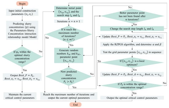
Figure 6.
The optimization process of CCPs based on the RZPGS algorithm.
3. Case Study and Results
3.1. Project Profile and Construction Data
To validate the application of the CSD’s optimization framework for CCPs based on hybrid machine learning, the CSD “Tianda” was deployed in a harbor dredging project, primarily tasked with silt removal for harbor construction, as illustrated in Figure 7. The initial slurry surface elevation in the construction area is approximately −11 m, requiring excavation to reach an elevation of −14 m, with a total project volume of approximately 402,000 m3. The SCADA system installed at the CSD collects various parameter data during the construction process, forming the basis for subsequent capacity prediction and optimization. All codes were developed using Python 3.9 on a computer equipped with an Intel CoreTM i7-1365UE CPU @ 4.90 GHz, featuring 10 cores and 12 threads. The soil composition within the construction area is clay and silty clay. However, the maximum concentration allowed in the design pipe is limited to 30%. Analyzing 20,000 sets of historical operating data collected by the SCADA system during the construction of the CSD determined that the optimal concentration range falls within the first 30% of the historical data. Consequently, the optimum SC range for this case is between 17.53% and 30%.
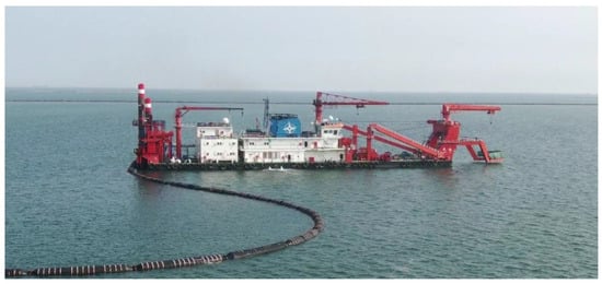
Figure 7.
“Tianda” CSD construction site.
Table 3 shows the parameter observations recorded by the CSD during the different construction periods, using the monitoring data from the SCADA system. The monitoring dataset comprised 256 dimensions and was automatically collected and stored at 8 s intervals. The construction monitoring data for the CSD exhibit high dimensionality, large volume, strong temporal correlation, significant variations, and substantial fluctuations. Due to the influence of uneven soil conditions on the performance of the cutter head, each monitored parameter depicted continuous changes, as illustrated in Figure 8.
Table 3.
Construction monitoring data of CSD obtained from the SCADA system.
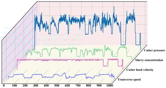
Figure 8.
The reamer cutting system monitoring data.
3.2. Model Performance Verification
In this investigation, the model was trained using 20,000 sets of randomly collected historical operating data obtained from the CSD construction through the SCADA system. Figure 9 depicts the data distribution for the transverse speed (), cutter head velocity (), and SC (), which are crucial to the investigation. The horizontal speed of the CSD remained consistent in both swing directions, and the cutter head velocity () exhibited fluctuations hovering around 30 rpm. After completing a transverse swing section, the cutter head would temporarily stop dredging operations during the forward hull advance until it reached the next dredging site. Consequently, during the hull’s advancement towards the next dredging points, both the transverse speed () and cutter head velocity () remained at 0 for a specific duration. This study primarily explores how variations in transverse speed () and cutter head velocity () influence the SC () during the construction process.
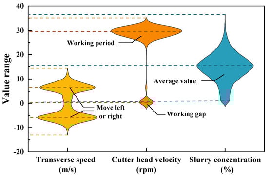
Figure 9.
The critical parameters value range.
The effectiveness of the Jaya–MLP combination algorithm was further validated by training the model on 20,000 sets of historical operational data obtained from the CSD. The training set was constructed with sample sizes of 3000, 6000, 9000, 12,000, 15,000, and 18,000 samples. To comprehensively assess the model’s performance, the test set comprising 1000 samples was employed, and the results are illustrated in Figure 10. The specific parameters configurations for the Jaya–MLP combined algorithm are outlined in Table 4. This model incorporates a ReLU activation function and has two hidden layers, encompassing 100 and 40 neurons, respectively.
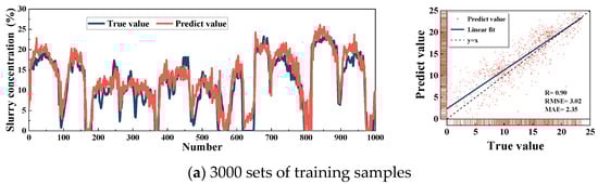
Figure 10.
Prediction performance of the Jaya–MLP model with various numbers of training sets.
Table 4.
The parameters of the Jaya–MLP model.
The Jaya–MLP model consistently followed the actual monitoring data across all six distinct sample sizes, with a robust overall goodness of fit and with correlation coefficients exceeding 0.9. Additionally, this model eliminated the need for workers to manually input intricate parameters, emphasizing its convenience for engineering practice and showcasing its predictive prowess for SC.
3.3. Multi-Parameter Sensitivity Analysis
After data preprocessing, an analysis was conducted to investigate the interaction between the transverse speed () and cutter head velocity () within the reamer cutting system. A multi-parameter sensitivity analysis was performed on the CCP combination to provide insights into the effect of the CCP adjustment. This analysis aimed to preliminary validate the coarse results of CCPs, providing an understanding of how parameter variations influenced the overall operational dynamics.
The transverse speed () was adjusted incrementally by 2 m/s, creating five sets of parameter adjustment schemes with respective speeds of + 2 m/s, + 4 m/s, + 6 m/s, + 8 m/s, and + 10 m/s. Furthermore, the cutter head velocity () was typically maintained within the range of 10–30 rpm based on the accumulated experience of the construction team. Monitoring data for the cutter head velocity () within this range indicated a gradient increase set at 2 rpm, resulting in five groups of parameter adjustments: + 2 rpm, + 4 rpm, + 6 rpm, + 8 rpm, and + 10 rpm.
A total of 25 experimental groups were generated through orthogonal experiments, conducted under consistent conditions for other factors. These groups were used to ascertain the effects of optimization and identify the optimal parameter adjustment combinations. In the construction parameters–SC interaction relationship model established earlier, two sets of construction areas (I and II) characterized by a high SC () were randomly selected. Additionally, two sets (III and IV) of construction areas with low SCs () were also randomly chosen for calculation. The outcomes of these calculations are detailed in Table 5.
Table 5.
SC prediction results after CCP adjustment.
The results revealed that various combinations of adjustment amplitudes for the transverse speed () and cutter head velocity () had varied effects on the SC during construction. The optimal adjustment effects, highlighted in a bold font among the construction areas (I, II, III, and IV), were observed under CCP combinations of ( + 2, + 2), ( + 8, + 2), ( + 2, + 2), and ( + 8, + 2). These preliminary findings underscored the significance of CCP optimization. To illustrate the impact of transverse speed (), four groups of orthogonal combination experiments corresponding to + 2 were selected for Figure 11. The average SC associated with the optimal CCP combination under each construction area was marked with a red star. It is evident that a 2 rpm increase in cutter head velocity () indicated that a minor adjustment in cutter head velocity () could be more effective in enhancing the overall concentration. The optimal effect for transverse speed () was observed within two distinct ranges: an increase of 2 m/s and an increase of 8 m/s, respectively. The observed optimization effects might vary depending on the specific construction areas. Therefore, operators should consider the specific construction environment and historical data when making judgements. This indicates that further refinement is necessary for the tuning of CCP optimization.
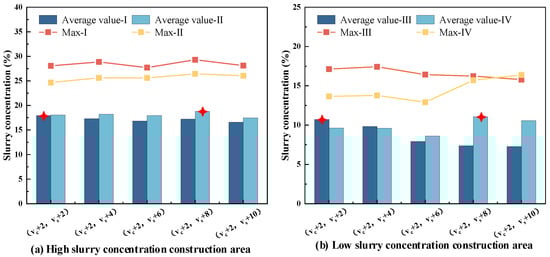
Figure 11.
Effect of transverse speed () on SC in multi-parameter sensitivity analysis.
To validate the optimization efficacy of this method, an effect analysis was conducted, selecting adjustments in the CCPs for construction SC data during a single lateral excavation process under construction areas IV. Figure 12 illustrates a comparison of the SC for CCPs in this construction section under the original construction parameters and the optimal optimization scheme. After implementing adjustments to the CCPs, there was a discernible enhancement in the SC, with an average increase of 22.5%. The maximum SC reached 15.72%, while the average SC was recorded at 14.05% during the stable construction stage. Significantly, the improvement effect was more pronounced in the initial construction stage than in the stable construction stage. The average SC increases from 4.02% to 8.87%, representing a remarkable surge of up to 120.65%. This suggested that appropriately increasing the transverse speed () and cutter head velocity () could effectively enhance the SC in low-concentration sections. However, it was worth noting that the achieved levels had not yet reached the optimal range (17.53–30%) specified for low-concentration construction areas.
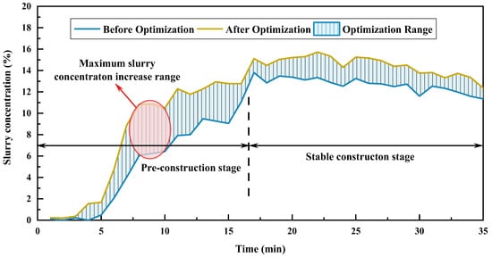
Figure 12.
The comparison involves evaluating the impact of the construction SC following CCP multi-parameter sensitivity analysis.
Therefore, the aforementioned approach facilitates the investigation of the correlation between adjusting CCPs and SCs during construction across diverse construction areas. The preliminary optimization outcomes were designed to enhance the SC during construction. However, there is still an opportunity for the further refinement of the precision of the CCPs, especially in low-concentration construction areas where achieving optimal effects proves challenging.
3.4. Optimization of Critical Control Parameters
To provide more accurate suggestions for the optimization of CCPs and further enhance the SC during construction, a meticulous examination was conducted on the SCADA system’s dataset, comprising 20,000 CSD construction history operation datasets and the construction record data that should have accumulated for approximately 44 h. The average SC during the construction period was recorded as 14.63%. Additionally, the average flow rate was determined to be 10,883.09 m3/h, with a maximum flow rate of 11,896.15 m3/h. After excluding a small number of construction data points that exceeded the permitted maximum concentration and flow rate limits, our analysis revealed that the optimal SC range is situated within the initial 30% of historical operational data, precisely spanning from 17.53% to 30%. This range was defined as the optimal SC set under these dredging conditions and corresponds to the optimal construction parameters illustrated in Figure 13.
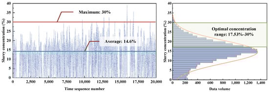
Figure 13.
The distribution of the SC and the range of the optimal concentration.
The timeliness of our framework is exemplified in Table 6, which presents a temporal comparison between the RZPGS algorithm and the conventional grid search algorithm. The calculation duration is contingent on factors such as data volume, algorithmic processes, and parameters, under the assumption of identical computer configurations. Both the RZPGS algorithm and the conventional grid search algorithm were configured to execute 50 iterations under defined parameter settings. To demonstrate the efficacy of the RZPGS algorithm in optimizing CCPs, the algorithm was applied to four distinct construction areas (high SC construction areas: I and II; low SC construction areas: III and IV), each comprising 150 sets for analysis. To emphasize the computational efficiency of the proposed method, a comparison was made with the grid search algorithm. The primary reasons for selecting the grid search algorithm for comparison are its simplicity, fast response time, and suitability for real-time optimization scenarios. Notably, the RZPGS algorithm consistently demonstrated superior optimization results, significantly enhancing the efficiency of CCPs optimization, with an average duration of 6.7 s. This represented a notable improvement, being 9.4 times faster than the grid search algorithm. Additionally, the computational duration was even shorter than the data acquisition interval of 8 s. Consequently, our method can meet the requisite temporal constraints for optimizing CCPs in CSD construction.
Table 6.
A time-based comparison between the RZPGS algorithm and the conventional grid search algorithm.
The dataset obtained from construction areas IV (low SC area) was used to explore the results of the autonomous optimization of CCPs. Figure 14 illustrates the impact of CCP adjustments on SC. It demonstrates the optimization effect achieved through the autonomous optimization process, where 150 time series numbers correspond to 150 sets of continuous construction collection data, representing 20 min of continuous construction collection data during the construction phase. The findings indicate that the mean SC during construction increased significantly by 27.4% after CCP optimization, reaching an average of 18.6%. This SC fell within the previously defined optimal range of [17.53%, 30%]. The figure illustrates that the optimization effect was particularly pronounced when the initial concentration was lower. It is noteworthy that in section of the construction site, as depicted in Figure 14, the SC improved significantly from 8.4% to 15.2%, an impressive increase of 81%. In regions with higher concentrations, the algorithm effectively maintained the original construction parameters. For example, in section , the initial SC was 20.3%, already within the optimal range [17.53%, 30%], so no further adjustments were deemed necessary for CCPs in this specific construction area.
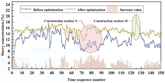
Figure 14.
The impact of CCP optimization on SC.
The optimization outcomes of the CCPs are visually presented in Figure 15. In the construction area, the average transverse speed () increased from 6.02 m/s to 6.54 m/s, with a notable maximum increase of 3.41 m/s. Similarly, the cutter head velocity () increased from 29.99 rpm to 30.81 rpm, with a recorded maximum increase of 2.03 rpm. This generally aligns with the findings obtained through multi-parameter sensitivity analysis.
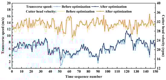
Figure 15.
The optimization results of CCPs.
Dredging production served as a crucial indicator of construction efficiency, with the results being depicted in Figure 16. At a construction duration of 20 min, the cumulative production increased from 447.27 m3 to 563.74 m3, representing a relative increase of 26.04%. This evidence demonstrates that the RZPGS algorithm effectively optimizes CCPs, providing operators with guidance for parameter adjustments and consequently enhancing dredging production.
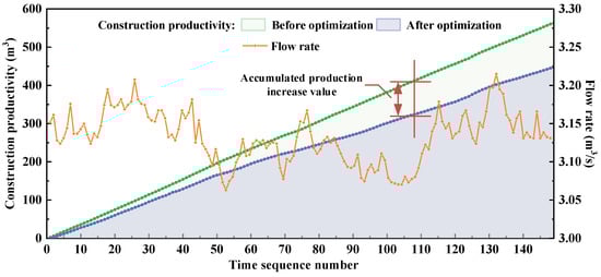
Figure 16.
Comparison of cumulative production before and after optimization of CCPs.
3.5. Practical Application Considerations
The optimization framework for CCPs in a CSD was introduced and analyzed based on the case study. The results illustrated that the optimization framework has streamlined parameter configuration and rapid optimization speed, making it highly suitable for CSD construction. However, certain issues were identified during the case study analysis.
Firstly, the optimization framework relies on a data-driven analysis of historical construction data from the continuous data stream of CSD operations. Given the prevalent geological composition, primarily characterized by clay and silty clay with relatively consistent soil quality, it is anticipated that the feedback for cutter head construction will concern the uniformity throughout the process. However, incorporating additional monitoring data on diverse soil qualities, including varying feedback on cutter head construction states (e.g., encountering rocks), during the model learning phase may necessitate the further refinement of the framework before implementation.
Secondly, the CSD is a sophisticated integrated system encompassing multiple subsystems, which requires the collaborative functioning of bow blowing and other systems during construction. Furthermore, a multitude of parameters collectively influence the efficiency of construction. Despite the abundance of 256-dimensional monitoring data, the monitoring data for the bow blowing system remains relatively limited. This discrepancy presents a challenge in the design and implementation of the monitoring system, potentially leading to the exclusion of CCPs within the bow blowing system in this study. Therefore, further investigation into coordinated parameters analysis, involving systems such as the reamer cutting system, SCADA system, transverse system, positioning system, slurry conveying system, bow blowing, and so on, is essential to achieve the synchronous optimization of additional control parameters throughout the CSD construction process.
Finally, due to the elevated construction costs associated with the CSD, the proposed optimization framework is currently limited to the research stage. Implementing the proposed optimization framework could impact the employment and salaries of construction technicians, potentially discouraging practical testing of CSD. It is anticipated that the application period will be extended, necessitating the continuous monitoring and testing of the framework to identify potential issues that may not have been previously anticipated. The ongoing process is designed to enhance the long-term feasibility of the proposed optimization framework.
4. Conclusions and Future Work
This study introduced an efficient productivity-aware control parameter optimization framework in a CSD. Firstly, the Jaya–MLP combined algorithm is employed to quickly establish a construction parameters–SC interaction relationship model to capture the slurry concentration during production. Secondly, a multi-parameter sensitivity analysis of CCPs is conducted to determine the preliminary coarse results. Finally, the RZPGS algorithm is employed to optimize the construction combination of the CSD, thereby obtaining more accurate results. The applicability of our approach is validated using monitoring data from the dredging operations of the “Tianda” CSD as a case study. Based on these findings, several conclusions can be drawn.
(1) The analysis of CSD construction revealed that the SC is a crucial indicator for assessing production efficiency. The transverse speed and cutter head velocity are considered as CCPs, and an efficient productivity-aware optimization framework for CCPs in the construction process was proposed.
(2) The construction parameters–SC interaction relationship model constructed by Jaya–MLP demonstrated a consistent fitting trend with the actual monitoring data, with a high overall goodness of fit and correlation coefficients exceeding 0.9. This indicated that the proposed model exhibited excellent predictive capacity and could accurately monitor the slurry concentration during the production. Subsequently, a multi-parameter sensitivity analysis was employed to determine the preliminary coarse results of CCP combination optimization. This method was applied to optimize CCPs in four construction areas, resulting in an increase in the cutter head velocity by 2 rpm. However, the optimal results for the transverse speed were achieved through two different increases: 2 m/s and 8 m/s, respectively. After optimization, a noticeable enhancement in the overall SC was observed compared to the pre-optimization state. The average SC exhibited a notable increase of 22.5%, with the maximum SC reaching 15.72%. Furthermore, during the period of the stable construction stage, the average SC achieved 14.05%. However, the multi-parameter sensitivity analysis still faced challenges with insufficient optimization accuracy and unsatisfactory optimization effects.
(3) The RZPGS algorithm was employed to further optimize CCPs, with the objective of enhancing calculation accuracy and reducing computation duration. The more accurate optimization results revealed that, compared to the conventional grid search algorithm, the RZPGS algorithm significantly enhanced the computational efficiency. The average optimization duration for the RZPGS algorithm was 6.7 s, representing a remarkable 9.4-fold increase in computational efficiency. Moreover, the optimization duration was shorter than the data acquisition interval of the SCADA system (8 s), indicating that CCPs could be optimized before the next set of monitoring data was read during the construction process. This would provide timely optimized results for construction workers. After the optimization of CCPs, the SC during the construction process consistently remained high within an expanded range of 27.4%, with the average SC reaching 18.6%, falling within the predetermined optimal SC range. These findings validated the effectiveness of our proposed automatic optimization framework, which provided operators with timely and appropriate guidance for adjusting CCPs during construction.
It should be noted that the proposed approach also has limitations for further improvement. On the one hand, the soil quality in the construction area does not exhibit significant variations in this study case. However, compared to slurry, the operation control methods of the cutter head structure differ when working under geological conditions such as high-strength rocks. Therefore, it is essential to conduct a thorough investigation to evaluate the necessity of improving the proposed framework. On the other hand, considering advancements in detection system technology, there may be opportunities to reduce the monitoring interval time, necessitating the faster optimization of CCPs in subsequent research.
Author Contributions
Conceptualization, R.L.; Methodology, R.L.; Software, R.L.; Validation, H.L., S.B. and Y.C.; Resources, H.L.; Data curation, S.B. and L.L.; Writing—original draft, R.L.; Writing—review & editing, R.L.; Visualization, H.L.; Supervision, R.L.; Project administration, R.L.; Funding acquisition, H.L. All authors have read and agreed to the published version of the manuscript.
Funding
This research was jointly funded by the China Postdoctoral Science Foundation (Grant No. 2023TQ0239) and the Major Science and Technology Project of the Ministry of Water Resources (Grant Nos. SKS-2022028 and SKS-2022147).
Data Availability Statement
Data are available from the authors by request.
Conflicts of Interest
Author Hao Liu was employed by PowerChina Zhongnan Engineering Corporation Limited. The remaining authors declare that the research was conducted in the absence of any commercial or financial relationships that could be construed as a potential conflict of interest.
References
- Erftemeijer, P.L.A.; Lewis, R.R.R. Environmental impacts of dredging on seagrasses: A review. Mar. Pollut. Bull. 2006, 52, 1553–1572. [Google Scholar] [CrossRef] [PubMed]
- Bai, S.; Li, M.C.; Kong, R.; Han, S.; Li, H.; Qin, L. Data mining approach to construction productivity prediction for cutter suction dredgers. Autom. Constr. 2019, 105, 102833. [Google Scholar] [CrossRef]
- Wei, C.Y.; Bai, H.N.; Wei, Y.; Ji, Z.; Liu, Z.H. Learning manipulation skills with demonstrations for the swing process control of dredgers. Ocean Eng. 2022, 246, 110545. [Google Scholar] [CrossRef]
- Wei, Y.; Wei, C.Y.; Yuan, B. Flow velocity stability control of slurry pipeline transportation of cutter suction dredgers. J. Nanjing Univ. Sci. Technol. 2021, 45, 332–337, 351. [Google Scholar] [CrossRef]
- Zhang, M.; Fan, S.D.; Zhua, H.H.; Han, S. Numerical simulation of solid-fluid 2-phase-flow of cutting system for cutter suction dredgers. Pol. Marit. Res. 2018, 25, 117–124. [Google Scholar] [CrossRef]
- Bai, Y.M.; Wang, D.S.; Wang, W. The swing control system design of cutter suction dredger based on predictive control. Navig. Chin. 2021, 44, 28–32, 38. [Google Scholar]
- Shang, G.; Xu, L.Y.; Tian, J.Z.; Cai, D.W. Productivity regression analysis of cutter suction dredger considering operating characteristics and equipment status. Proc. Inst. Mech. Eng. Part M J. Eng. Marit. Environ. 2023, 237, 406–419. [Google Scholar] [CrossRef]
- Vancauwenbergh, L.; Vandepitte, D.; Moens, D.; Vanneste, G.; Vercruijsse, P. Reconstruction and analysis of the torsional excitation force component of a cutter suction dredger in hard rock conditions. In Proceedings of the International Conference on Noise and Vibration Engineering (ISMA)/International Conference on Uncertainty in Structural Dynamics (USD), Leuven, Belgium, 7–9 September 2020; pp. 2699–2713. [Google Scholar]
- Vijayan, K.; Barik, C.R.; Sha, O.P. Shock transmission through universal joint of cutter suction dredger. Ocean Eng. 2021, 233, 109185. [Google Scholar] [CrossRef]
- Wei, C.Y.; Wei, Y.; Ji, Z. Model predictive control for slurry pipeline transportation of a cutter suction dredger. Ocean Eng. 2021, 227, 108893. [Google Scholar] [CrossRef]
- Xiong, T.; Wang, J.X.; Wei, W.; Jiang, P.; Zhang, Y.J. Numerical simulation of rock cutting process with cutter-suction dredger. Navig. Chin. 2022, 45, 69–75. [Google Scholar]
- Shang, G.; Xu, L.Y.; Tian, J.Z.; Cai, D.W.; Xu, Z.; Zhou, Z. A real-time green construction optimization strategy for engineering vessels considering fuel consumption and productivity: A case study on a cutter suction dredger. Energy 2023, 274, 127326. [Google Scholar] [CrossRef]
- Fu, J.K.; Tian, H.J.; Song, L.G.; Li, M.C.; Bai, S.; Ren, Q.B. Productivity estimation of cutter suction dredger operation through data mining and learning from real-time big data. Eng. Constr. Archit. Manag. 2021, 28, 2023–2041. [Google Scholar] [CrossRef]
- Jena, D.P.; Panigrahi, S.N. Estimating acoustic transmission loss of perforated filters using finite element method. Measurement 2015, 73, 1–14. [Google Scholar] [CrossRef]
- Martins, R.S.; de Aquino, G.S.; Martins, M.F.; Ramos, R. Sensitivity analysis for numerical simulations of disturbed flows aiming ultrasonic flow measurement. Measurement 2021, 185, 110015. [Google Scholar] [CrossRef]
- Üstünyagiz, E.; Nielsen, C.V.; Tiedje, N.S.; Bay, N. Combined numerical and experimental determination of the convective heat transfer coefficient between an AlCrN-coated Vanadis 4E tool and Rhenus oil. Measurement 2018, 127, 565–570. [Google Scholar] [CrossRef]
- Wang, B.; Fan, S.D.; Chen, Y.; Zheng, L.Y.; Zhu, H.H.; Fang, Z.L.; Zhang, M. The replacement of dysfunctional sensors based on the digital twin method during the cutter suction dredger construction process. Measurement 2022, 189, 110523. [Google Scholar] [CrossRef]
- Wang, B.; Fan, S.D.; Jiang, P.; Zhu, H.H.; Xiong, T.; Wei, W.; Fang, Z.L. A novel method with stacking learning of data-driven soft sensors for mud concentration in a cutter suction dredger. Sensors 2020, 20, 6075. [Google Scholar] [CrossRef]
- Yao, M.H.; Wang, Y.L.; Shang, J.; Zhang, J.Y. Study on the cutter suction dredgers productivity model and its optimal control. In Proceedings of the International Conference on Modeling, Simulation and Optimization Technologies and Applications (MSOTA), Xiamen, China, 18–19 December 2016; pp. 81–85. [Google Scholar] [CrossRef]
- Han, S.; Li, H.; Li, M.C.; Tian, H.J.; Qin, L.; Yu, Y.; Ma, J. Intelligent short-term forecasting for mud concentration in CSD dredging construction. Ocean Eng. 2022, 266, 113151. [Google Scholar] [CrossRef]
- Yang, K.; Yuan, J.L.; Xiong, T.; Wang, B.; Fan, S.D. A novel principal component analysis integrating long short-term memory network and its application in productivity prediction of cutter suction dredgers. Appl. Sci. 2021, 11, 8159. [Google Scholar] [CrossRef]
- Lang, X.; Wu, D.; Mao, W.A. Physics-informed machine learning models for ship speed prediction. Expert Syst. Appl. 2024, 238, 121877. [Google Scholar] [CrossRef]
- Parkes, A.I.; Savasta, T.D.; Sobey, A.J.; Hudson, D.A. Power prediction for a vessel without recorded data using data fusion from a fleet of vessels. Expert Syst. Appl. 2022, 187, 115971. [Google Scholar] [CrossRef]
- Elhaki, O.; Shojaei, K.; Mehrmohammadi, P. Reinforcement learning-based saturated adaptive robust neural-network control of underactuated autonomous underwater vehicles. Expert Syst. Appl. 2022, 197, 116714. [Google Scholar] [CrossRef]
- Bai, S.; Li, M.C.; Lu, Q.R.; Fu, J.K.; Li, J.F.; Qin, L. A new measuring method of dredging concentration based on hybrid ensemble deep learning technique. Measurement 2022, 188, 110423. [Google Scholar] [CrossRef]
- Li, M.C.; Lu, Q.R.; Bai, S.; Zhang, M.X.; Tian, H.J.; Qin, L. Digital twin-driven virtual sensor approach for safe construction operations of trailing suction hopper dredger. Autom. Constr. 2021, 132, 103961. [Google Scholar] [CrossRef]
- Li, M.C.; Kong, R.; Han, S.; Tian, G.P.; Qin, L. Novel method of construction-efficiency evaluation of cutter suction dredger based on real-time monitoring data. J. Waterw. Port Coast. Ocean Eng. 2018, 144, 05018007. [Google Scholar] [CrossRef]
- Bai, S.; Li, M.C.; Lu, Q.R.; Tian, H.J.; Qin, L. Global time optimization method for dredging construction cycles of trailing suction hopper dredger based on Grey System Model. J. Constr. Eng. Manag. 2022, 148, 04021198. [Google Scholar] [CrossRef]
- Wang, W.; Shen, Y.C.; Wang, L.Y.; Wang, D.S.; Bai, Y.M. Design of dredging process control system for cutter suction dredger. In Proceedings of the 33rd Chinese Control and Decision Conference (CCDC), Kunming, China, 22–24 May 2021; pp. 5932–5937. [Google Scholar] [CrossRef]
- Li, J.Y.; Shi, Y.Y.; Rao, K.P.; Zhao, K.Y.; Xiao, J.F.; Xiong, T.; Huang, Y.Z.; Huang, Q.B. The design and analysis of double cutter device for hinge and suction dredger based on feedback control method. Appl. Sci. 2022, 12, 3793. [Google Scholar] [CrossRef]
- Lan, Y.; Hu, J.W.; Huang, J.H.; Niu, L.K.; Zeng, X.H.; Xiong, X.Y.; Wu, B. Fault diagnosis on slipper abrasion of axial piston pump based on Extreme Learning Machine. Measurement 2018, 124, 378–385. [Google Scholar] [CrossRef]
- Wei, C.Y.; Wang, H.; Bai, H.A.; Ji, Z.; Liu, Z.H. PPLC: Data-driven offline learning approach for excavating control of cutter suction dredgers. Eng. Appl. Artif. Intell. 2023, 125, 106708. [Google Scholar] [CrossRef]
- Wang, B.; Fan, S.D.; Jiang, P.; Xing, T.; Fang, Z.L.; Wen, Q. Research on predicting the productivity of cutter suction dredgers based on data mining with model stacked generalization. Ocean Eng. 2020, 217, 108001. [Google Scholar] [CrossRef]
- Gondia, A.; Siam, A.; El-Dakhakhni, W.; Nassar, A.H. Machine learning algorithms for construction projects delay risk prediction. J. Constr. Eng. Manag. 2020, 146, 04019085. [Google Scholar] [CrossRef]
- Bai, S.; Li, M.C.; Song, L.G.; Ren, Q.B.; Qin, L.; Fu, J.K. Productivity analysis of trailing suction hopper dredgers using stacking strategy. Autom. Constr. 2021, 122, 103470. [Google Scholar] [CrossRef]
- Lai, H.H.; Chang, K.H.; Lin, C.L. A novel method for evaluating dredging productivity using a data envelopment analysis-based technique. Math. Probl. Eng. 2019, 2019, 5130835. [Google Scholar] [CrossRef]
- Wei, C.Y.; Ni, F.S.; Chen, X.J. Obtaining human experience for intelligent dredger control: A reinforcement learning approach. Appl. Sci. 2019, 9, 1769. [Google Scholar] [CrossRef]
- Yang, J.B.; Ni, F.S.; Wei, C.Y. A BP neural network model for predicting the production of a cutter suction dredger. In Proceedings of the 3rd International Conference on Material, Mechanical and Manufacturing Engineering (IC3ME), Guangzhou, China, 27–28 June 2015; pp. 1221–1226. [Google Scholar] [CrossRef]
- JTJ 319-1999; The Technical Code of Dredging Engineering. China Communications Press: Beijing, China, 1999.
- Wang, B.; Fan, S.D.; Jiang, P.; Chen, Y.; Zhu, H.H.; Xiong, T. Cutting state estimation and time series prediction using deep learning for cutter suction dredger. Appl. Ocean Res. 2023, 134, 103515. [Google Scholar] [CrossRef]
- Li, W.; Wang, F.X.; Jiang, J.A. Parameter identification, verification and simulation of the CSD transport process. In Proceedings of the 11th International Conference on Advanced Computational Intelligence (ICACI), Guilin, China, 7–9 June 2019; pp. 118–123. [Google Scholar] [CrossRef]
- Liu, Z.; Lin, Y.T.; Cao, Y.; Hu, H.; Wei, Y.X.; Zhang, Z.; Lin, S.; Guo, B.N. Swin transformer: Hierarchical vision transformer using shifted windows. In Proceedings of the 18th IEEE/CVF International Conference on Computer Vision (ICCV), Electr Network, Montreal, QC, Canada, 11–17 October 2021; pp. 9992–10002. [Google Scholar] [CrossRef]
- Kim, T.; Adali, T. Approximation by fully complex multilayer Perceptrons. Neural Comput. 2003, 15, 1641–1666. [Google Scholar] [CrossRef]
- Castro, J.L.; Mantes, C.J.; Benítez, J.M. Neural networks with a continuous squashing function in the output are universal approximators. Neural Netw. 2000, 13, 561–563. [Google Scholar] [CrossRef]
- Pedregosa, F.; Varoquaux, G.; Gramfort, A.; Michel, V.; Thirion, B.; Grisel, O.; Blondel, M.; Prettenhofer, P.; Weiss, R.; Dubourg, V. Scikit-learn: Machine learning in Python. J. Mach. Learn. Res. 2011, 12, 2825–2830. [Google Scholar]
- Uzlu, E. Application of Jaya algorithm-trained artificial neural networks for prediction of energy use in the nation of Turkey. Energy Sources Part B 2019, 14, 183–200. [Google Scholar] [CrossRef]
- Jothi, G.; Inbarani, H.H.; Azar, A.T.; Devi, K.R. Rough set theory with Jaya optimization for acute lymphoblastic leukemia classification. Neural Comput. Appl. 2019, 31, 5175–5194. [Google Scholar] [CrossRef]
- Yu, K.J.; Liang, J.J.; Qu, B.Y.; Chen, X.; Wang, H.S. Parameters identification of photovoltaic models using an improved JAYA optimization algorithm. Energy Conv. Manag. 2017, 150, 742–753. [Google Scholar] [CrossRef]
- Lujan-Moreno, G.A.; Howard, P.R.; Rojas, O.G.; Montgomery, D.C. Design of experiments and response surface methodology to tune machine learning hyperparameters, with a random forest case-study. Expert Syst. Appl. 2018, 109, 195–205. [Google Scholar] [CrossRef]


Disclaimer/Publisher’s Note: The statements, opinions and data contained in all publications are solely those of the individual author(s) and contributor(s) and not of MDPI and/or the editor(s). MDPI and/or the editor(s) disclaim responsibility for any injury to people or property resulting from any ideas, methods, instructions or products referred to in the content. |
© 2024 by the authors. Licensee MDPI, Basel, Switzerland. This article is an open access article distributed under the terms and conditions of the Creative Commons Attribution (CC BY) license (https://creativecommons.org/licenses/by/4.0/).