Defining and Mitigating Flow Instabilities in Open Channels Subjected to Hydropower Operation: Formulations and Experiments

Abstract

A thorough literature review was conducted on the effects of free surface oscillation in open channels, highlighting the risks of the occurrence of positive and negative surge waves that can lead to overtopping. Experimental analyses were developed to focus on the instability of the flow due to constrictions, gate blockages, and the start-up and shutdown of hydropower plants. A forebay at the downstream end of a tunnel or canal provides the right conditions for the penstock inlet and regulates the temporary demand of the turbines. In tests with a flow of 60 to 100 m³/h, the effects of a gradually and rapidly varying flow in the free surface profile were analyzed. The specific energy and total momentum are used in the mathematical characterization of the boundaries along the free surface water profile. A sudden turbine stoppage or a sudden gate or valve closure can lead to hydraulic drilling and overtopping of the infrastructure wall. At the same time, a PID controller, if programmed appropriately, can reduce flooding by 20–40%. Flooding is limited to 0.8 m from an initial amplitude of 2 m, with a dissipation wave time of between 25 and 5 s, depending on the flow conditions and the parameters of the PID characteristics.

1. Introduction

Hydropower plants with forebays and intake channels are crucial for the use of water to generate electricity. These facilities are designed to efficiently control the flow of water and ensure a steady and controlled supply of pumped storage hydroelectricity. The forebay is a retention basin where the water is temporarily stored before it enters the penstock. It helps to regulate fluctuations in water flow and sediment and provides a stable and clean source of water for the turbines. The intake channel then directs the water from the springs to the tunnels and then to the forebay.

This type of hydropower utilization is particularly effective in areas with natural watercourses. It enables both power generation and water management for drinking water supply and irrigation as a multi-purpose pumped storage power plant, contributing to renewable energy goals with minimal environmental impact. The integration of these components ensures efficient operation, reduced water losses, and the ability to cope with changing water conditions. This makes hydropower plants with forebays, intake canals, and tunnels an important part of a sustainable energy infrastructure.

Currently, over 81% of global energy consumption comes from fossil fuels, even though they are polluting the environment and resources are being depleted [1]. While energy demand continues to rise, renewable sources only contribute around 13.7%. Among renewables, hydropower is one of the most efficient and reliable, accounting for 2.5% of global energy and 15.9% of electricity generation [2]. The most important guidelines for the design of hydropower plants are presented in [3].

Concerns related to the stable methods for determining structural damping by frequency response function curve fitting techniques in the context of water level control or power plant operation can be found in [4]. Waves in fluids and fluid mechanics form the basis for this study of open channel flows [5,6]. If the hydropower circuits have flow elements in open channels, momentum analysis in hydraulic jumps and bores is essential [7,8]. Positive surge propagation and undular bores (Favre waves) in open channels are investigated by [9,10,11].

The coupling between fluctuations at the free surface, velocity fluctuations, and turbulent Reynolds stresses during the upstream propagation of positive surge waves, bores, and compression waves, as well as the influence of different shapes and depths on the formation of tidal bores, are analyzed by [12,13]. The propagation of a positive surge in an asymmetric channel is described by [14]. The narrowing of the channel cross-section and the application of the specific energy in open channels to different forms of channel narrowing have been analyzed by [15,16,17].

An interesting study on numerical simulations of the detour properties of a channel is presented by [18]. Local head losses in the lateral diversion of open channels with different cross-sectional shapes and the analysis of the effects of channel width variations on the turbulent flow are presented in [19,20].

Relevant recent studies have investigated the impact of unsteady flow from hydropower stations on water levels in multi-approach channels, which pose risks to ship safety. The studies employ one-dimensional and two-dimensional hydrodynamic models to simulate water level fluctuations at channel entrances and the lower lock head of a ship lift. The analysis considers factors like initial water surface elevation, base flow, flow amplitude, regulation time, and the location of hydropower stations, effectively identifying unfavorable conditions [21]. Benefits and challenges along natural channels are analyzed by [22], making references to the huge Three Gorges project in the Yangtze River by improving the waterway channel. A short-term multi-objective optimal operation of reservoirs is enhanced by [23] with the objective to maximize the benefits of hydropower operation. Free surface flow basic hydraulic formulations are conducted in terms of specific flow energy and total momentum analyses. Open-channel flows are an especially important mode of fluid mechanics for civil and environmental engineers. One needs to predict the flow rates and water depths that result from a given channel geometry, whether natural or artificial, and a given wet-surface roughness. Water is the studied fluid, and the flow in the channel is mostly a 1D-type flow due to the length being much higher than the width of the channel. Thus open-channel flows are generally turbulent, three-dimensional, sometimes unsteady, and often quite complex. This research presents some simple engineering theories and experimental correlations for steady flow in straight channels of regular geometry associated with hydropower conveyance systems [24,25]. On the other hand, [26] presents several formulations to estimate the length of hydraulic jump in rectangular open channels with variable slopes. Dynamic effects associated with small hydropower systems with long hydraulic circuits are studied by [27], enhancing the surges that can happen in open channels induced by turbine stoppage or start-up during normal operation. The need for a forebay to guarantee the minimum submergence at the water intake and the surge waves damping propagation to upstream channels requires a specific element such as a forebay, which makes the transition between channels and penstocks. The water level regulation requires some controllers that can be obtained by Mathlab Simulink 10.1. A hydroturbine governor system (HTGS) is a nonlinear system coupled with hydraulic, mechanical, and electrical subsystems. When a small load disturbance signal appears, the governor adjusts the turbine guide vanes according to the signal difference to balance the power system. Fluctuations in system parameters, such as the discharge, forebay water level, and turbine rotational speed, from an initial stable state to another one, indicate that the whole system is under a transient process. Moreover, hydropower plants with long headrace or tailrace tunnels are normally equipped with forebay or surge tanks to control the water hammer pressure propagation. However, as the water level fluctuates over a long period and has a slow decay rate, the stability characteristics of hydropower plants become more complex due to the interaction between the oscillations in the HTGS and free surface flows. If the system design parameters are unreasonable or the tuning of the governor is inappropriate, the oscillations of the system will be unstable during a load disturbance. The stability and quality of regulation are significant to the safety of the hydropower plant and even to the power system [28,29,30].

2. Methodology, Theoretical Formulations, and Experiments

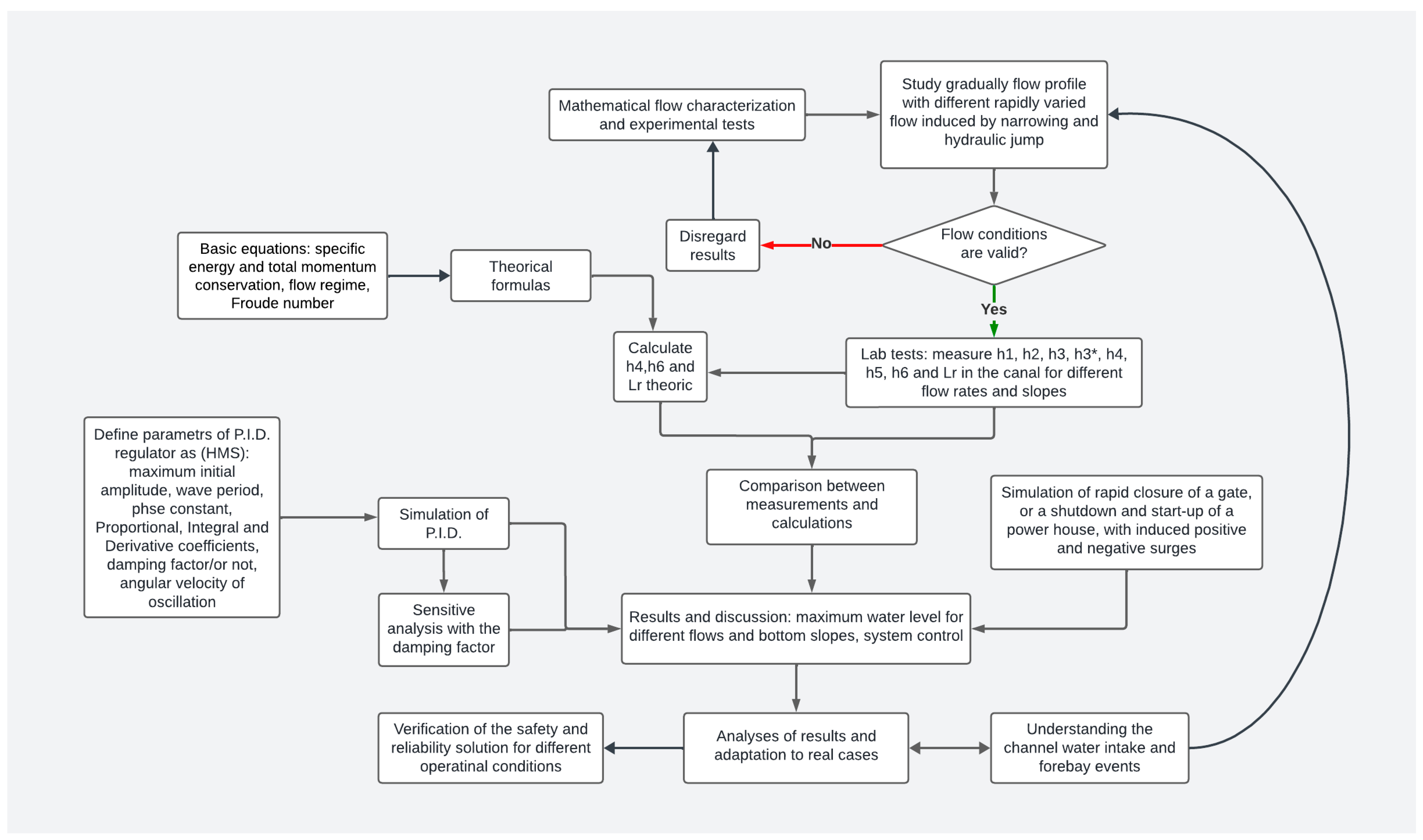
2.1. Methodology

Positive and negative fluctuations triggered by hydropower plants have a significant impact on water levels in open rivers with multiple tributaries. In this study, theoretical developments and experimental analyzes were presented to improve the hazards of the hydrodynamic flow model that can destabilize the channel flow conditions due to constrictions, gate obstructions, and the start-up or shutdown of hydropower plants/pumps.

Sudden fluctuations in turbine discharge can lead to fluctuations in water levels along a detour channel. A canal water intake such as “Levadas” on Madeira Island and a forebay forming the transition between the Covão tunnel and the Socorridos penstock can be used as a regulating reservoir [4] to mitigate possible fluctuations and improve the response of the canal to changes in turbine discharge. In addition, they can also serve as protection against silt and floating debris and as a sedimentation basin. Figure 1, therefore, shows the integrated methodology for free surface flow in hydropower plant components, such as water intake channels and forebays, with different boundary conditions.

Surge waves are associated with the operation of the system. When the hydropower plant requires an increased discharge, the water level drops rapidly and can exceed the supply capacity of the canal. Conversely, when the power plant shuts down, a hydraulic bore can propagate upstream. At the same time, the canal continues to supply the forebay, which can lead to secondary surge waves and overtopping of the canal walls.

A forebay positioned at the downstream end of a tunnel or canal (Figure 2) is sized based on the following considerations:

• Ensure adequate conditions for the water intake of the penstock and associated equipment (e.g., trash rack, sluices, gates, and weirs) while meeting the minimum flooding criteria;
• Limiting flow fluctuations along the canal due to operating changes in the hydropower station;
• Providing a control function to meet the temporary needs of the turbines regardless of the flow regime.

To better understand what can happen in a water intake channel or tunnel as an integral part of hydraulic infrastructures, water conduit tunnels are widely used in hydropower projects (Figure 2) [3]. To regulate the flow, there are some gates, weirs, constrictions, or even spillways which control the flow through the critical water depth, which is the transition between subcritical and supercritical flow.

The water depth profile along an open channel changes with the flow conditions, e.g., from a steady flow (i.e., constant wall roughness, depth, and slope) to a gradually changing (can be modeled in a one-dimensional representation) or rapidly changing (with strongly curved streamlines and multidimensional) and surge-like bore. Positive and negative surge flows triggered by hydropower plants have a significant influence on the water level.

This must be calculated as part of a problem that can occur with wave movements, such as the formation of a hydraulic jump at the transition from supercritical to subcritical flow. In a hydropower plant, many phenomena can jeopardize or even endanger the upstream channels and water intakes by restricting the safe free surface flow through the formation of bores and, in some cases, possibly leading to channel overflow. An experimental analysis was developed to simulate the hydrodynamic flow effect in the channel caused by a narrow constriction/enlargement or by the start-up or shutdown of hydropower plants. In this section, several experiments were carried out in the channel of the IST Hydraulics Laboratory, in which different flow patterns and hydraulic jumps occurred.

The contraction flow was used to study the flow from the Levadas canal water intake to the Covão tunnel and the forebay. In these cases, the water can pass from the subcritical flow at the upstream section to the supercritical flow at the downstream section, increasing the flow velocity. A hydraulic jump then occurs so that the subcritical flow reaches a state of equilibrium again. A sudden interruption in turbine operation can cause an additional hydraulic bore to propagate upstream. These events can trigger secondary oscillation waves, possibly leading to overtopping of the channel walls. On the other hand, if the flow rate in the turbine is increased, the supply capacity of the canal may be exceeded.

To avoid the problems associated with the operation of the turbines, the Socorridos multipurpose system has a forebay between the Covão tunnel and the penstock connecting Covão to Socorridos.

A special investigation was developed in the laboratory, and experiments were analyzed in a channel for different singularities, flow velocities, and slopes in order to define better the flow behavior in open channels that can occur in waterways, water intakes, and forebays of hydroelectric plants.

2.2. Theory and Formulations

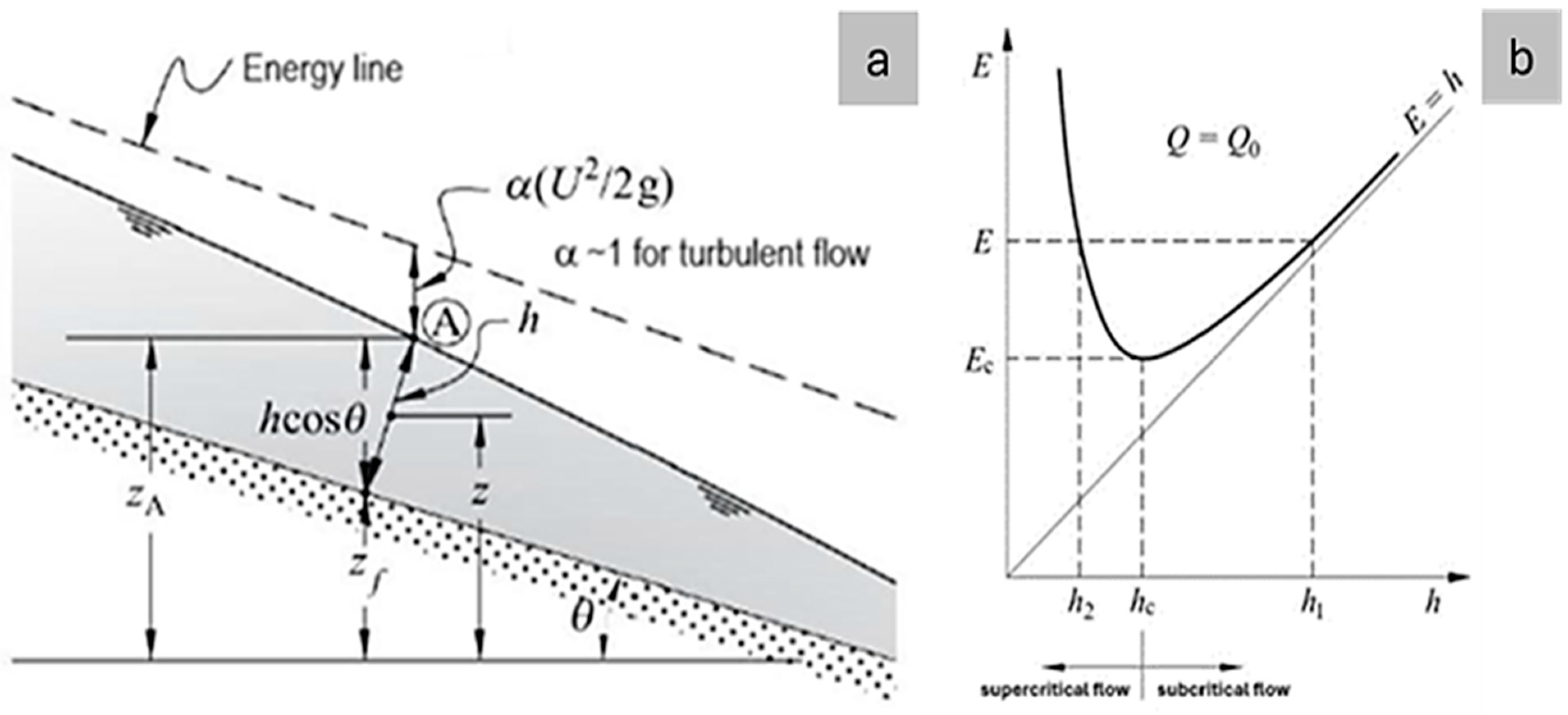
2.2.1. Bernoulli Equation and Specific Energy

For flows with a free surface, the total head (H) is given by Equation (1), where z is the vertical elevation of the water, α is the Coriolis coefficient, U is the velocity, and g is the gravity acceleration.

$$\mathrm{H}=\mathrm{z}+\frac{\mathsf{\alpha }{\mathrm{U}}^2}{2\mathrm{g}}$$

(1)

The vertical elevation of the water is composed of two components (Equation (2)), where h is the water depth, z_f the canal bottom elevation, and θ is the angle formed by the tangent of the longitudinal profile of the channel bottom with the horizontal.

$$\mathrm{z}=\mathrm{hcos}\mathsf{\theta }+{\mathrm{z}}_{\mathrm{f}}$$

(2)

The specific energy (E) for a certain flow rate can be calculated using Equation (3).

$$\mathrm{E}=\mathrm{hcos}\mathsf{\theta }+\mathsf{\alpha }{\displaystyle \frac{{\mathrm{Q}}_0^2}{2{\mathrm{gS}}^2}}$$

(3)

This equation can be represented as a function of the water depth and the specific energy (Figure 3) [24].

As observed, the curve has two asymptotes. In the first case, the depth of the water tends towards zero; in the second case, the depth of the water tends towards infinity because the velocity tends towards zero. The lowest point of this function corresponds to the minimum specific energy (E_c) in which the flow can take place. If the flow has this energy, it is a critical flow. The respective water depth associated with these conditions is called the critical water depth (h_c).

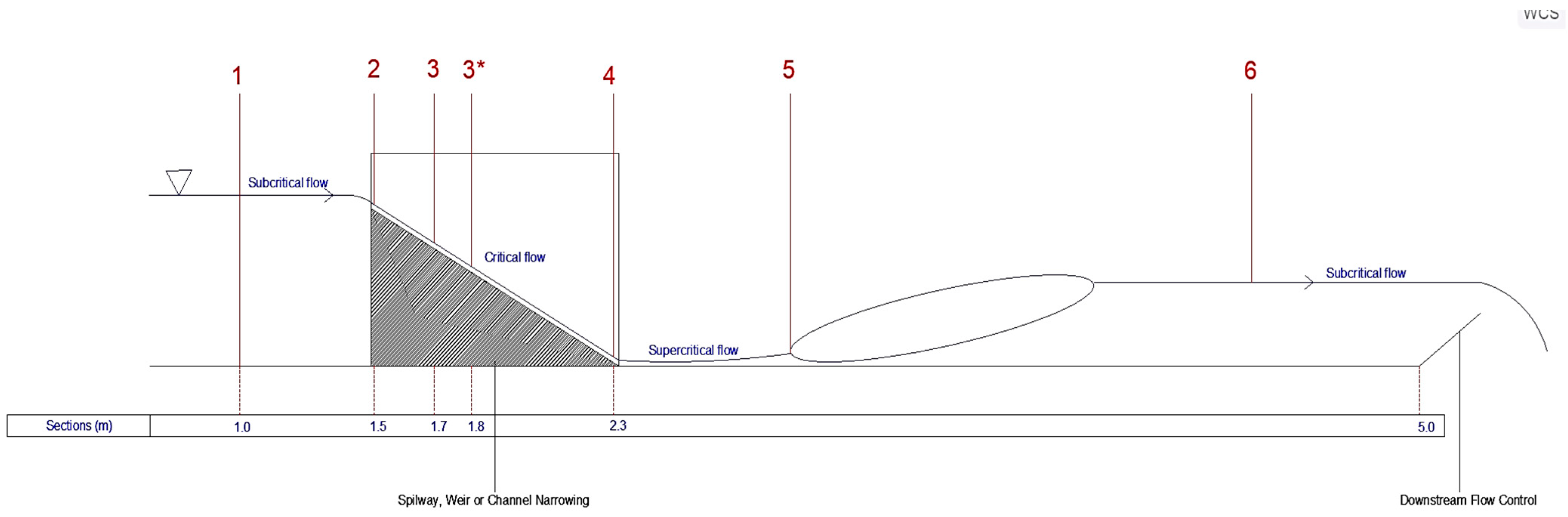
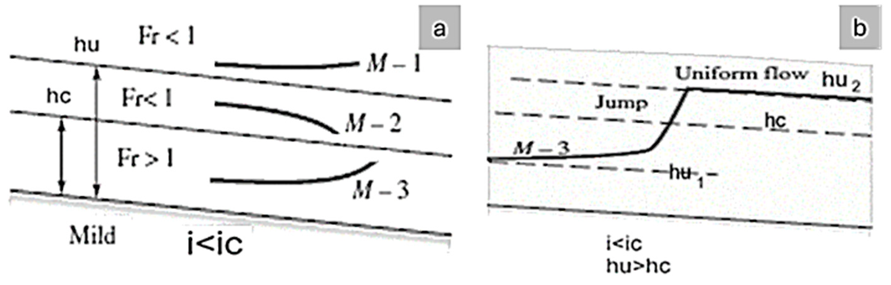
2.2.2. Supercritical, Critical, and Subcritical Flow

The condition of the critical flow is obtained, recurring to Equations (4) and (5). The S corresponds to the flow cross-section area.

$${\displaystyle \frac{\mathrm{dE}}{\mathrm{dh}}}={\displaystyle \frac{\mathrm{dh}}{\mathrm{dh}}}+{\displaystyle \frac{\mathrm{d}}{\mathrm{dh}}}\left({\displaystyle \frac{{\mathrm{Q}}_0^2}{2{\mathrm{gS}}^2}}\right)={\displaystyle \frac{\mathrm{dh}}{\mathrm{dh}}}+{\displaystyle \frac{\mathrm{d}}{\mathrm{dS}}}\left({\displaystyle \frac{{\mathrm{Q}}_0^2}{2{\mathrm{gS}}^2}}\right){\displaystyle \frac{\mathrm{dS}}{\mathrm{dh}}}=0$$

(4)

$${\displaystyle \frac{\mathrm{dE}}{\mathrm{dh}}}={\displaystyle \frac{\mathrm{dh}}{\mathrm{dh}}}+{\displaystyle \frac{{\mathrm{Q}}_0^2}{2\mathrm{g}}}{\displaystyle \frac{\mathrm{d}}{\mathrm{dS}}}\left({\displaystyle \frac{1}{{\mathrm{S}}^2}}\right){\displaystyle \frac{\mathrm{dS}}{\mathrm{dh}}}=1-{\displaystyle \frac{{\mathrm{Q}}_0^2}{2\mathrm{g}}}{\displaystyle \frac{2\mathrm{S}}{{\mathrm{S}}^4}}{\displaystyle \frac{\mathrm{dS}}{\mathrm{dh}}}=1-{\displaystyle \frac{{\mathrm{Q}}_0^2}{{\mathrm{gS}}^3}}{\displaystyle \frac{\mathrm{dS}}{\mathrm{dh}}}=0$$

(5)

Considering dS/dh~B, the flow rate is given for a specific critical section (Equation (6)).

$${\mathrm{Q}}_0=\sqrt{\mathrm{g}}{\mathrm{S}}_{\mathrm{c}}\sqrt{{\displaystyle \frac{{\mathrm{S}}_{\mathrm{c}}}{{\mathrm{B}}_{\mathrm{c}}}}}$$

(6)

The variation in the specific energy per unit length can be calculated using Equation (7):

$${\displaystyle \frac{\mathrm{d}}{\mathrm{dS}}}(\mathrm{hcos}\mathsf{\theta }+{\displaystyle \frac{{\mathsf{\alpha }\mathrm{U}}^2}{2\mathrm{g}}})=-\mathrm{J}+\mathrm{sen}\mathsf{\theta }$$

(7)

where J is the head loss per unit length.

For flows with a specific energy greater than that occurring in the critical flow, there are two water depths for the same specific energy. The flow is described as supercritical if the water depth is less than the critical water depth. On the other hand, if the water depth is above the critical water depth, the flow is referred to as subcritical. High velocities are observed in the first case and slow velocities in the second case.

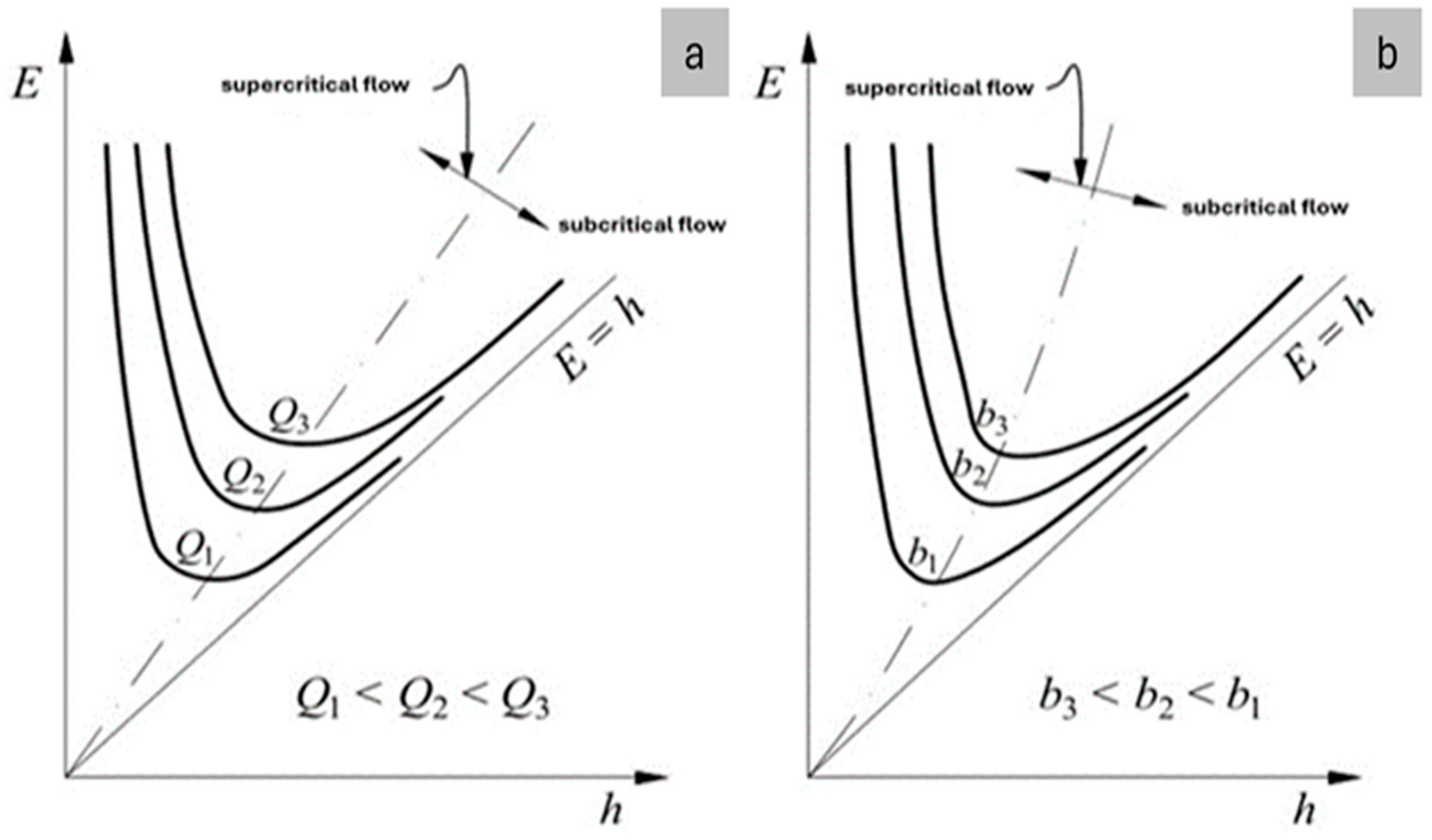
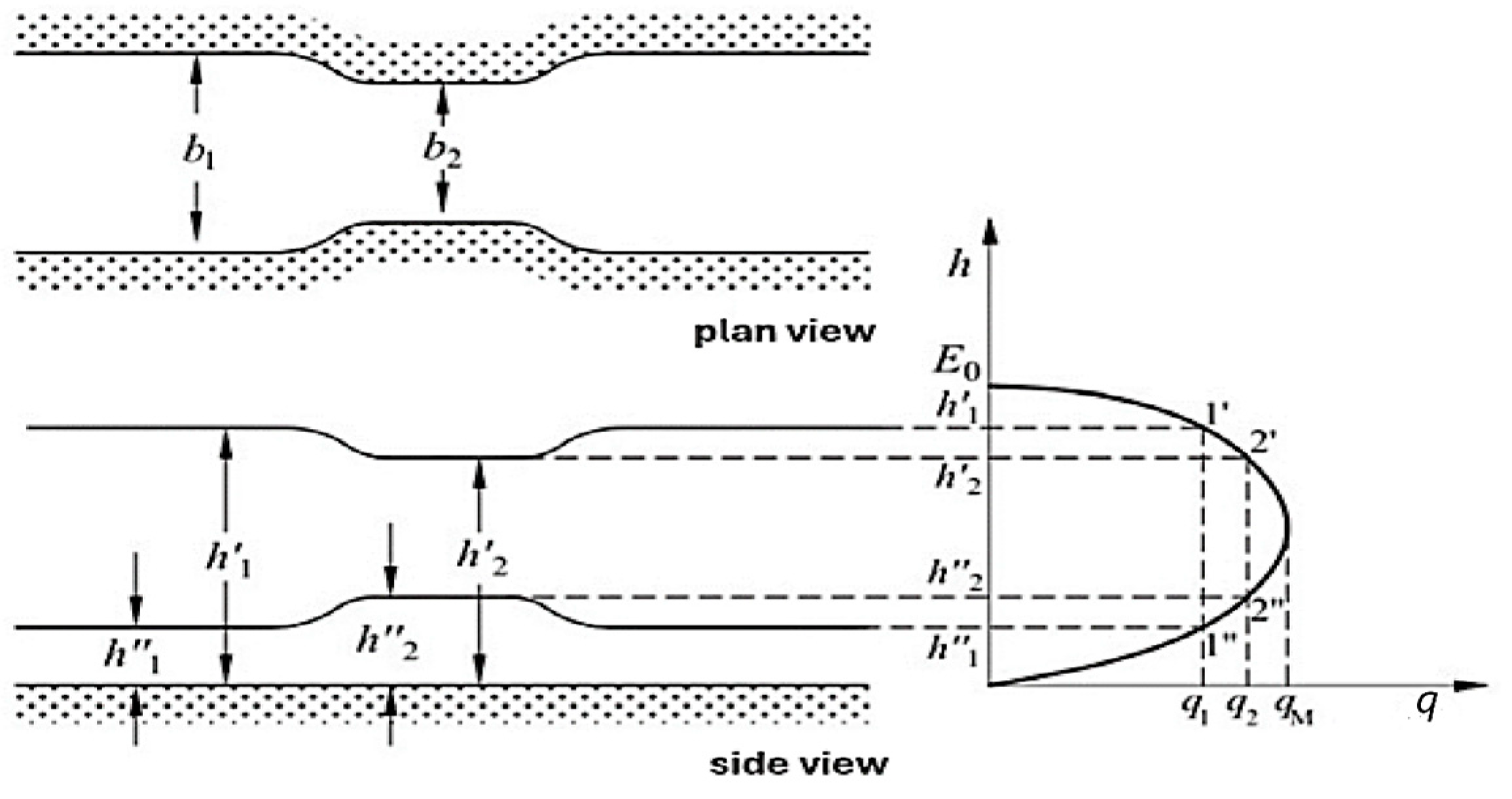
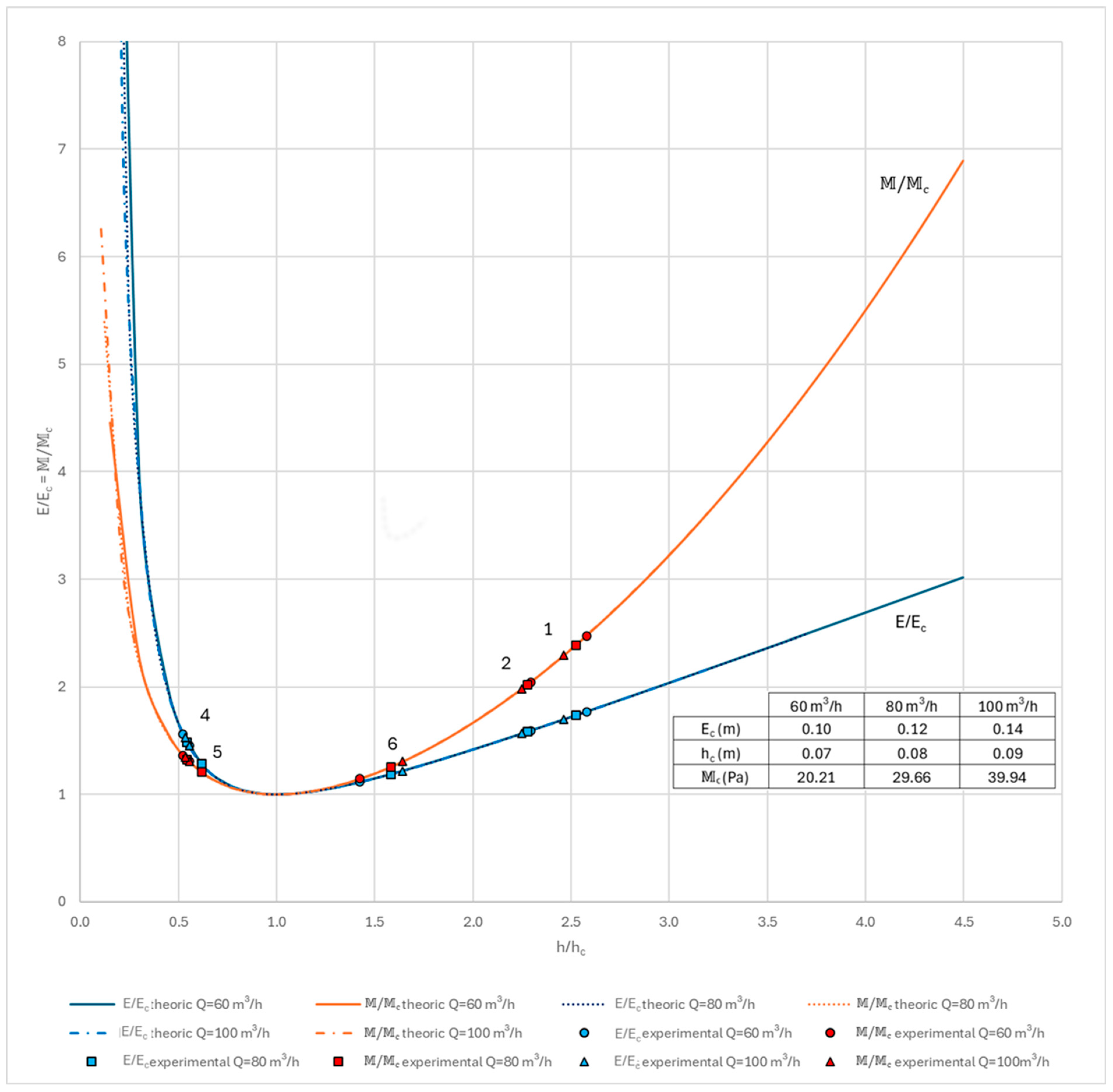
2.2.3. Influence of the Flow Rate and the Width on the Progression of E = E(h) Curves

The variation in the flow rate (Figure 4a) and the bottom-width (b) of the canal (Figure 4b) can induce different curves.

For the same water depth, the specific energy tends to increase as the flow rates increase (Figure 3a). For different sections, the specific energy decreases as the bottom-width of the channel (b) increases, assuming, for this case, a constant flow rate and a trapezoidal channel shape (Figure 3b). Increasing the channel width leads to a reduction in velocity and, consequently, to a lower specific energy for the same water depth.

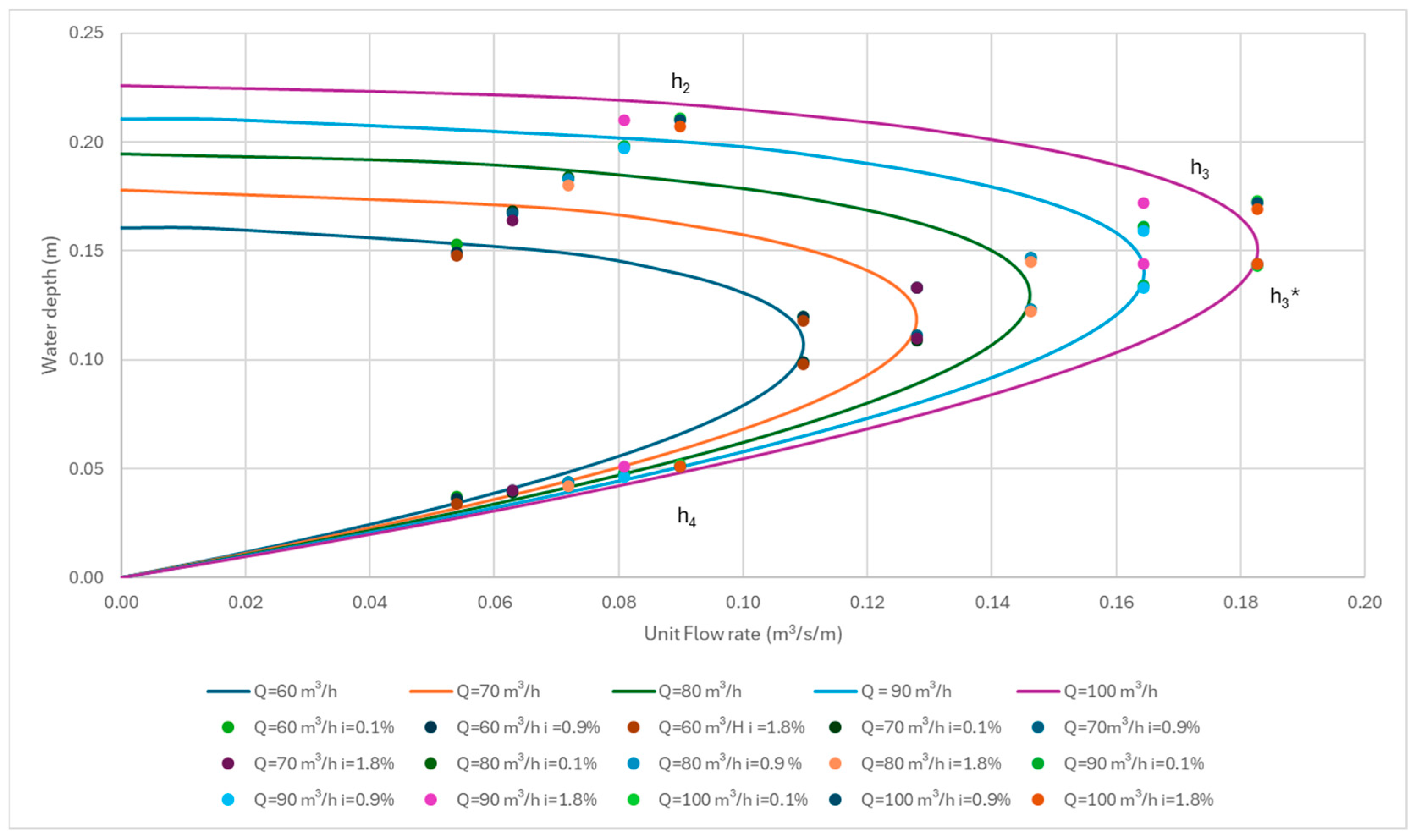
2.2.4. Maximum Flow Rate for E = E0

Figure 5a shows the change in flow rate for different specific energies with the same cross-section. The maximum flow rates increase as the specific energy increases. The dashed and dotted lines represent the geometric location of the critical points for each specific energy. Figure 5b shows the influence of the channel width on the maximum flow rate for a constant specific energy.

The analysis of Figure 5b shows that the maximum flow rate increases with increasing channel width. It is also important to note that the maximum flow rate occurs at the same critical water depth for all widths. For rectangular cross-sections, the critical water depth is given by Equation (8).

$${\mathrm{h}}_{\mathrm{c}}={\displaystyle \frac{2}{3}}{\mathrm{E}}_0$$

(8)

The critical energy for the same rectangular cross-section and the maximum flow rate (Q_M) achieved for each width can be calculated using Equations (9) and (10).

$${\mathrm{E}}_{\mathrm{c}}=1.5\sqrt[3]{{\displaystyle \frac{{\mathrm{Q}}_{\mathrm{M}}^2}{{\mathrm{gb}}^2}}}$$

(9)

$${\mathrm{Q}}_{\mathrm{M}}=\sqrt{{\displaystyle \frac{\mathrm{g}}{{1.5}^3}}}{\mathrm{bE}}_{\mathrm{c}}^{3/2}=0.385\mathrm{b}\sqrt{2\mathrm{g}}{\mathrm{E}}_{\mathrm{c}}^{3/2}$$

(10)

In these sections, the specific energy is determined, applying Equation (11), where S_c is the critical cross-section area.

$${\mathrm{E}}_{\mathrm{c}}={\mathrm{h}}_{\mathrm{c}}+{\displaystyle \frac{{\mathrm{Q}}_{\mathrm{M}}^2}{2{\mathrm{gS}}_{\mathrm{c}}^2}}$$

(11)

Taking Equation (10) into account, it is possible to calculate the maximum flow relative flow rate per unit width (q_M) given by Equation (12),

$${\mathrm{q}}_{\mathrm{M}}={\mathrm{h}}_{\mathrm{c}}\sqrt{2\mathrm{g}\left({\mathrm{E}}_0-{\mathrm{h}}_{\mathrm{c}}\right)}$$

(12)

The specific energy can now be written as a function of the unit flow rate (Equation (13)).

$${\mathrm{E}}_0=\mathrm{h}+{\displaystyle \frac{{\mathrm{q}}^2}{2{\mathrm{gh}}^2}}$$

(13)

Equation (12) is very useful for channels with width change and bottom rise (Figure 6), as the specific energy does not depend on the width. In this case, it was assumed that the specific energy is the same throughout the channel constriction.

In Figure 6, the width of the canal decreases from b₁ to b₂. At a width of b1, there are two operating points, 1′ and 1″, on the curve h = h(q), which correspond to a subcritical and supercritical flow, respectively. If the width is b₂, the flow rate per unit increases since b₂ < b₁. For the same specific energy, there are two new flow regimes, 2′ and 2″, for a subcritical and supercritical flow, respectively.

There is a minimum width compatible with the flow that corresponds to the critical flow for a given E₀ value, which can be calculated using Equation (14).

$${\mathrm{b}}_{\min }={\displaystyle \frac{\mathrm{Q}}{{\mathrm{q}}_{\mathrm{M}}}}$$

(14)

2.2.5. Slope Influence and Froude Number

The slope in a channel (i) can determine the type of uniform flow that can be generated. The critical slope leads to a flow with a uniform water depth (h_u) corresponding to the critical water depth. Supercritical and subcritical flows are observed at positive slopes greater and less than the critical slope, respectively. With negative and zero slopes, the uniform flow is never achieved. The ratio between twice the kinetic energy and the potential energy, calculated from the bottom of the channel, is represented by the Froude number (F_r), where m is the mass of fluid (Equation (15)).

$${\mathrm{F}}_{\mathrm{r}}={\displaystyle \frac{2\frac{1}{2}{\mathrm{mU}}^2}{\mathrm{mgh}}}={\displaystyle \frac{{\mathrm{U}}^2}{\mathrm{gh}}}$$

(15)

The Froude number can only be calculated for rectangular cross-sections using Equation (16), and it depends on the average flow water depth (h_m).

$${\mathrm{F}}_{\mathrm{r}}={\displaystyle \frac{\mathrm{U}}{\sqrt{{\mathrm{gh}}_{\mathrm{m}}\cos \mathsf{\theta }}}}$$

(16)

The value of the Froude number makes it possible to determine the type of flow that is present in a channel at a particular time instant.

$F_r=1$, for critical flow;

$F_r<1$, for subcritical flow;

$F_r>1$, for supercritical flow.

The change in water depth per unit length can be calculated based on Equations (7) and (16) via Equation (17).

$${\displaystyle \frac{\mathrm{dh}}{\mathrm{dx}}}={\displaystyle \frac{\mathrm{i}-\mathrm{J}}{1-{\mathrm{Fr}}^2}}$$

(17)

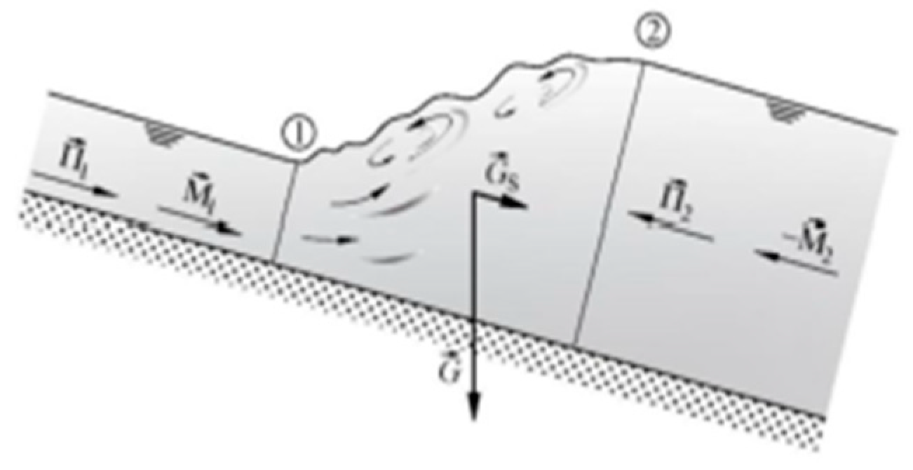
2.2.6. Conservation of Total Momentum in a Hydraulic Jump

A hydraulic jump is a phenomenon that occurs when water transitions from supercritical flow to subcritical flow. This transition results in a considerable loss of energy. The forces that occur during a hydraulic jump are shown in Figure 7.

The total momentum ($\mathbb{M}$) is defined by Equation (18) and results from the sum of the hydrostatic pressure ($\pi )$ and the linear momentum M in a specific cross-section. The $\gamma$ represents the specific weight of the fluid, and h_g represents the depth of the center of gravity.

$$\mathbb{M}=\mathsf{\pi }+\mathrm{M}={\mathsf{\gamma }\mathrm{Sh}}_{\mathrm{g}}+{\displaystyle \frac{{\mathsf{\gamma }\mathrm{Q}}^2}{\mathrm{gS}}}$$

(18)

The total momentum conservation results for prismatic channels and low θ (Equation (19)).

$${\displaystyle \frac{\mathrm{d}\mathbb{M}}{\mathrm{ds}}}=\mathsf{\gamma }\mathrm{S}\left(\mathrm{i}-\mathrm{J}\right)$$

(19)

Since the average shear stress compensates for the weight of the fluid, the total momentum between the upstream and downstream sections of the hydraulic jump is kept constant (Equation (20)):

$${\mathbb{M}}_1={\mathbb{M}}_2$$

(20)

Knowing the water depth in the upstream section of the hydraulic jump (h₁), it is possible to calculate the water depth in the downstream section (h₂). These water depths are called conjugate depths because they correspond to the same total momentum. The h₁ occurs in a supercritical flow, while h₂ corresponds to a subcritical flow.

Based on Equation (20), the relationship between the conjugated depths can be calculated (Equation (21)) for a non-submerged hydraulic jump.

$${\displaystyle \frac{{\mathrm{h}}_2}{{\mathrm{h}}_1}}={\displaystyle \frac{1}{2}}\left(\sqrt{1+8{\mathrm{F}}_{\mathrm{r}1}^2}-1\right)$$

(21)

Like this relationship, it is possible to obtain the relationship between h₁ and h₂ (Equation (22)).

$${\displaystyle \frac{{\mathrm{h}}_1}{{\mathrm{h}}_2}}={\displaystyle \frac{1}{2}}\left(\sqrt{1+8{\mathrm{F}}_{\mathrm{r}2}^2}-1\right)$$

(22)

2.2.7. Head Loss in a Hydraulic Jump

The head loss in a hydraulic jump (Δ_Er) is obtained by subtracting the specific energy in the upstream section (E₁) of the hydraulic jump from the specific energy in the downstream section of the hydraulic jump (E₂) (Equation (23)).

$$\Delta {\mathrm{E}}_{\mathrm{r}}={\mathrm{E}}_1-{\mathrm{E}}_2={\mathrm{h}}_1+{\displaystyle \frac{{\mathrm{U}}_1^2}{2\mathrm{g}}}-\left({\mathrm{h}}_2+{\displaystyle \frac{{\mathrm{U}}_2^2}{2\mathrm{g}}}\right)$$

(23)

For rectangular channels, the head loss is calculated using (Equation (24)).

$$\Delta {\mathrm{E}}_{\mathrm{r}}={\displaystyle \frac{{\left({\mathrm{h}}_2-{\mathrm{h}}_1\right)}^3}{4{\mathrm{h}}_2{\mathrm{h}}_1}}$$

(24)

Based on Equation (20), the head loss is function of the average velocity (U) using Equation (25).

$$\Delta {\mathrm{E}}_{\mathrm{r}}={\displaystyle \frac{{\left({\mathrm{U}}_1-{\mathrm{U}}_2\right)}^2}{2\mathrm{g}}}-{\displaystyle \frac{{\left({\mathrm{h}}_2-{\mathrm{h}}_1\right)}^2}{{\mathrm{h}}_2}}$$

(25)

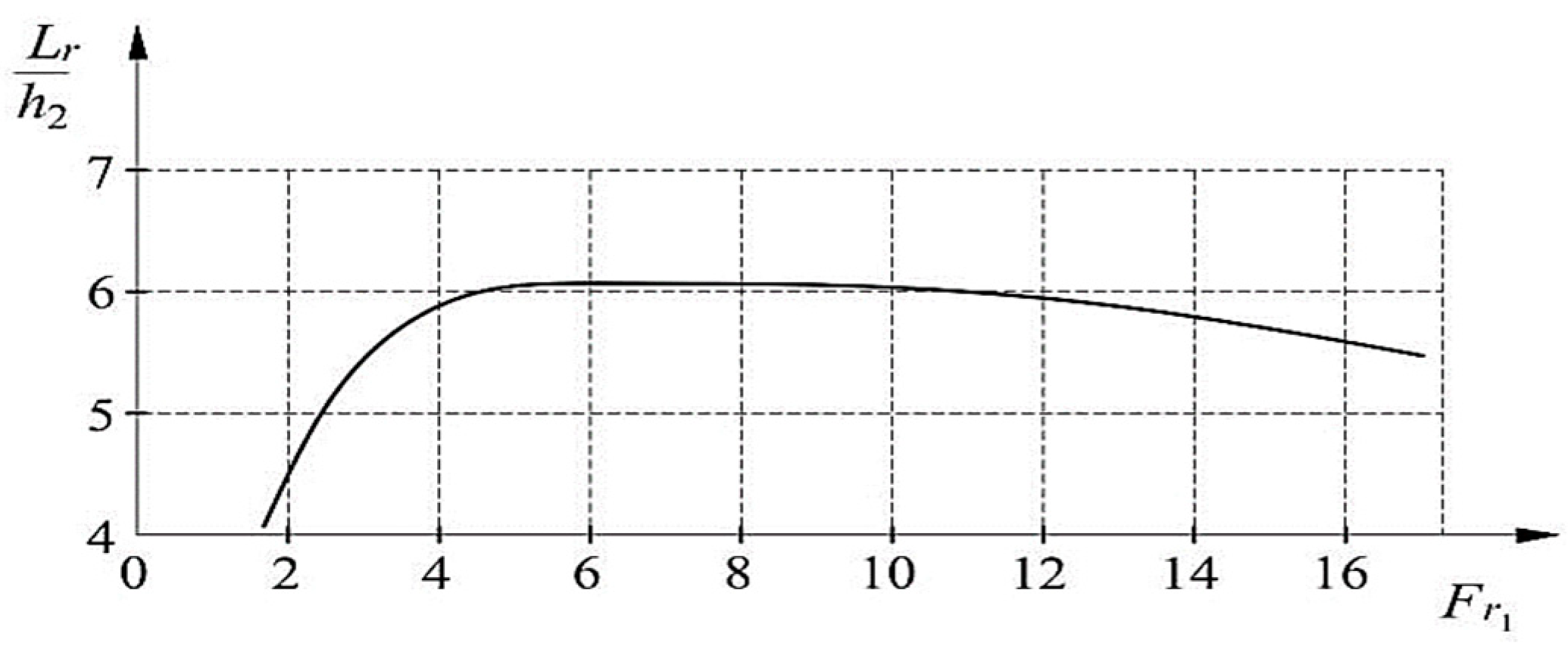
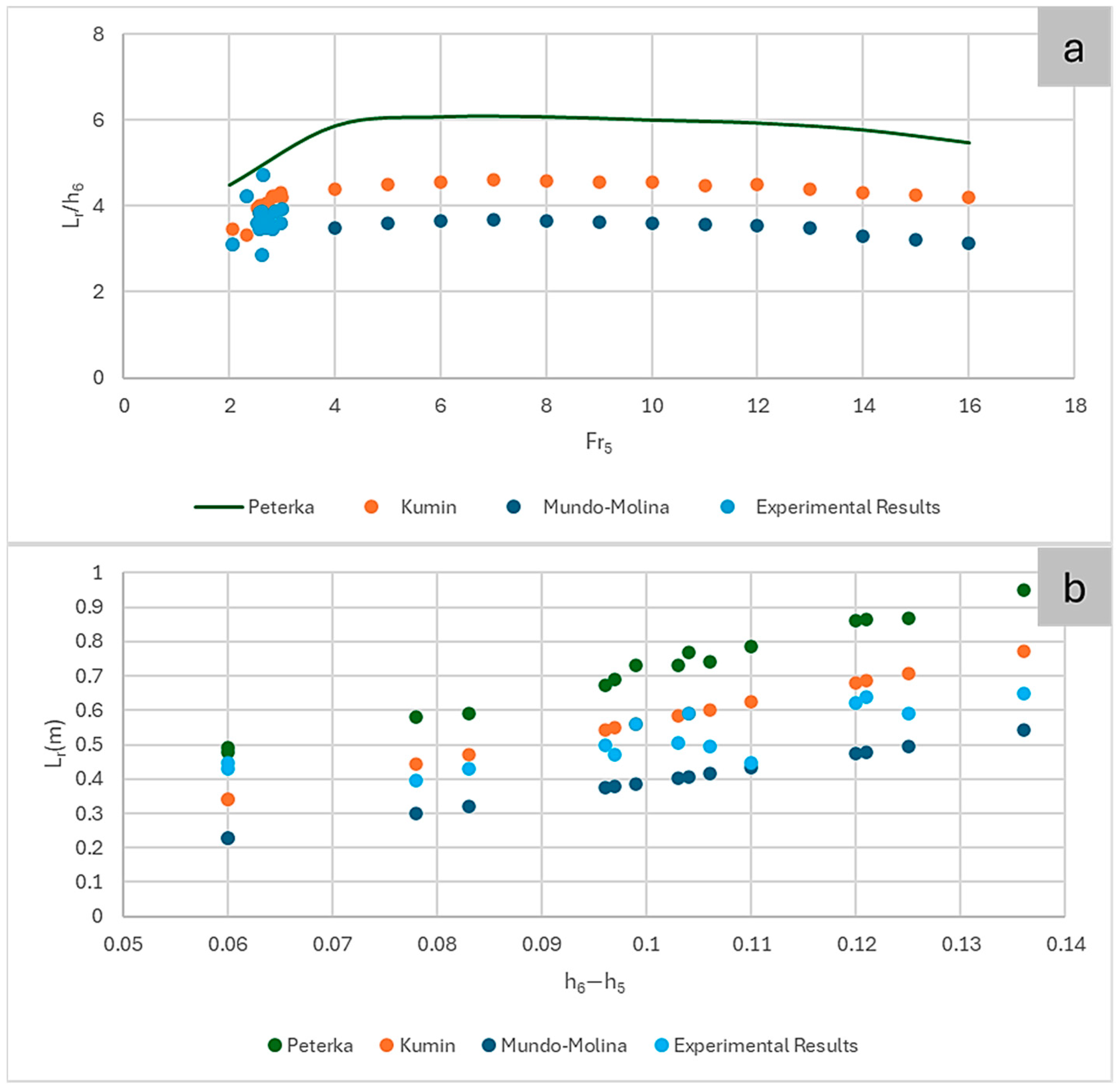
2.2.8. Hydraulic Jump Length

The length of the hydraulic jump (L_r) is the distance between its upstream and downstream sections. In these sections, there is a lot of turbulence and surface waves, which make it difficult to determine the average depth of the flow. The upstream section corresponds to the section where the depth of the current begins to increase. However, the downstream section is more difficult to identify. To determine the water depth in these two sections, it is advisable to take at least three measurements along the cross sections and then calculate the arithmetic mean of the water depth in each case. Figure 8 shows a curve that relates the L_r/h₂ to the F_r1, which was created by Peterka (1974).

The curve rises from L_r/h₂ equal to 4.4 to L_r/h₂ equal to 6 and then remains practically constant until F_r~12. This curve can only be used for high values of L_r/h₂. Other researchers defined new equations to determine the length of the hydraulic jump for low values of L_r, which are more suitable and effective for tests in the laboratory environment. Equations (26) and (27) show the estimations of Kumin and Mundo-Molina, respectively [25]

$${\mathrm{L}}_{\mathrm{r}}=5.67\left({\mathrm{h}}_2-{\mathrm{h}}_1\right)$$

(26)

$${\mathrm{L}}_{\mathrm{r}}=4.5456{\left({\mathrm{h}}_2-{\mathrm{h}}_1\right)}^{1.0657}$$

(27)

The equation formulated by [25] can only be applied for 1.2 < F_r1 < 5 and $0.11<{\displaystyle \frac{h_1}{b}}<$ 0.28.

2.2.9. Function $\mathbb{M}=\mathbb{M}\left(\mathrm{h}\right)$ for Q = Q₀

A function correlating $\mathbb{M}$, Q, and h in a three-dimensional space (see Equation (28)) makes it possible to analyze the relationship between M and a constant flow rate, and the following Equation (28) is obtained.

$${\mathrm{F}}_{\mathrm{M}}\left(\mathbb{M},\mathrm{h},\mathrm{Q}\right)=0$$

(28)

By intersecting the previous expression with a plane Q = Q₀, Equation (29) is obtained. This one is very similar to the one obtained for specific energy for a constant flow rate (Equation (3)).

$$\mathbb{M}=\mathsf{\gamma }\left({\mathrm{Sh}}_{\mathrm{g}}+{\displaystyle \frac{{\mathrm{Q}}_0^2}{\mathrm{gS}}}\right)$$

(29)

The representation of Equation (29) is illustrated in Figure 9.

The curve $\mathbb{M}=\mathbb{M} \left(h\right)$ has two asymptotes if h tends towards 0 and infinity. In the first case, when h tends towards 0, $\mathbb{M}$ tends towards infinity and the curve is asymptotic to the axis $\mathbb{M}\mathbb{M}$. On the other hand, if h tends to infinity, $\mathbb{M}$ tends to the assymptote of γShg. There is a minimum in the curve $\mathbb{M}=\mathbb{M} \left(h\right)$, which corresponds to the flow with the minimum total momentum for a flow velocity equal to Q₀. With the derivation of the total momentum according to h, Equation (30) is obtained.

$${\displaystyle \frac{\partial \mathbb{M}}{\partial \mathrm{h}}}=\mathsf{\gamma }\left({\mathrm{Sh}}_{\mathrm{g}}+{\displaystyle \frac{{\mathrm{Q}}_0^2}{\mathrm{gS}}}\right)$$

(30)

By establishing the relationship between the previous formula and the derivative of the specific energy to h, Equation (31) is obtained:

$${\displaystyle \frac{\partial \mathbb{M}}{\partial \mathrm{E}}}=\mathsf{\gamma }\mathrm{S}$$

(31)

From this formula, it follows that the minimal of the functions E/E_c and $\mathbb{M}/{\mathbb{M}}_{\mathrm{c}}$ coincide with the critical flow, for the minimum specific energy and the minimum total momentum for a given flow rate.

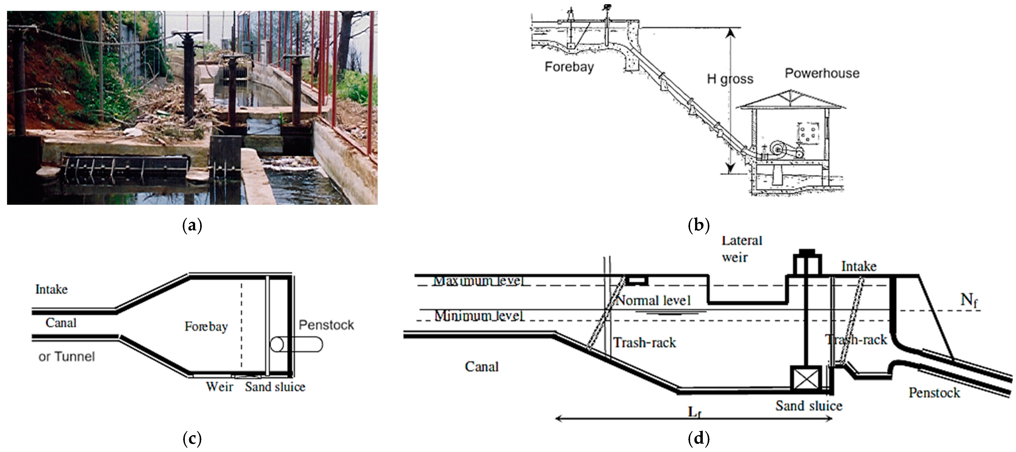
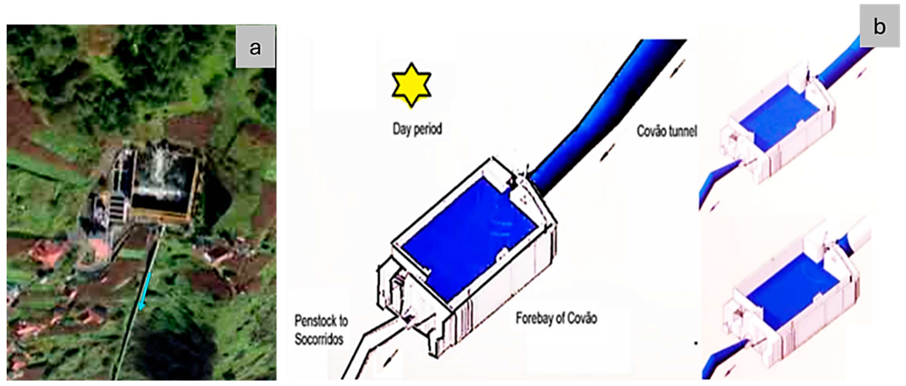
2.2.10. Forebay

The forebay in a hydropower plant is usually located between a canal/tunnel and a penstock, as shown in Figure 2c,d. These structures are built to ensure minimal flooding, to minimize flow fluctuations in the upstream channel, and to avoid transient demands due to extreme turbine operation (sudden stops and high hydropower flow rates). Three types of flows (steady, gradually fluctuating, and rapidly fluctuating) can be observed along the channel, depending on the downstream conditions. Without a forebay, the water can flood the canal walls. However, the formation of a hydraulic bore due to a flow reduction can affect its efficiency. On the other hand, when the water level decreases, air can enter the system, causing numerous compressions and expansions inside the penstock.

A hydraulic bore in a free surface flow, in particular a hydraulic jump, can be described with the aid of the Saint-Venant equations (Equations (32) and (33)) [25] and the correlation between the Froude numbers (Equation (35)) based on the conservation of total momentum, and it forms when the bore is higher than 20% of the initial level [3].

$${\displaystyle \frac{\partial \mathrm{U}}{\partial \mathrm{t}}}+{\displaystyle \frac{\partial \mathrm{F}\left(\mathrm{U}\right)}{\partial \mathrm{x}}}=\mathrm{D}\left(\mathrm{U}\right)$$

(32)

where U, F(U), and D(U) are the following vectors:

$$\mathrm{U}=\left[\mathrm{S}\mathrm{Q}\right]\mathrm{F}\left(\mathrm{U}\right)=\left[\mathrm{Q}{\displaystyle \frac{{\mathrm{Q}}^2}{\mathrm{S}}}+\mathrm{gSh}\right]\mathrm{D}\left(\mathrm{U}\right)=\left[\mathrm{gS}\left(\mathrm{i}-\mathrm{J}\right)\right]$$

(33)

and x = distance along the canal axis (m); t = time (s); S = cross-section flow area (m²); Q = flow rate (m³/s);

Another type of wave, the so-called Favre waves, which correspond to the secondary oscillations above the hydraulic jump, can form above the surge waves (Figure 10a,b). The increase in water depth caused by these waves (Equation (35)) can be calculated by deriving the Saint-Venant Equations.

The height of the side walls of the channel is designed based on the depth of the Favre waves with a minimum limit of ~0.15 m for the wall freeboard. The surge depth, above the initial canal water level, which is formed when the flow is completely interrupted downstream, can be determined using the Feifel formula (Equation (34)) [3,25].

$${\mathrm{F}}_{\mathrm{r}1}={\mathrm{F}}_{\mathrm{ro}}+\sqrt{{\displaystyle \frac{1}{2}}\left(1+{\displaystyle \frac{{\mathrm{h}}_1}{{\mathrm{h}}_2}}\right)}$$

(34)

The height of the side walls of the channel is designed based on the depth of the Favre waves with a minimum limit of ~0.15 m for the wall freeboard. The surge depth, above the initial canal water level, which is formed when the flow is controlled downstream, can be determined using the Feifel formula (Equation (35)).

$$\mathsf{\Delta }\mathrm{h}={\displaystyle \frac{{{\mathrm{U}}_1}^2}{2\mathrm{g}}}+\sqrt{{\left({\displaystyle \frac{{{\mathrm{U}}_1}^2}{2\mathrm{g}}}\right)}^2+2{\displaystyle \frac{{{\mathrm{U}}_1}^2}{2\mathrm{g}}}{\displaystyle \frac{{\mathrm{S}}_1}{{\mathrm{b}}_2}}}$$

(35)

Large areas of the forebay can reduce the height of the water level, which affects the upstream part of the channel where Δh surge depth is above the initial water level.

By increasing the horizontal forebay area, the bore height Δh, which spreads upstream of the detour channel, is attenuated.

To ensure the maximum head of the power plant and the power generated, an automatic water level is usually set in the forebay. On the upstream side of the detour channel, the flow changes can be caused either by natural fluctuations or by a lock function. On the downstream side, the main source of level fluctuations is the change in turbine discharge. In this case, the water level control can be based on a PID controller (Proportional, Integral, and Derivative) to ensure stable and efficient control.

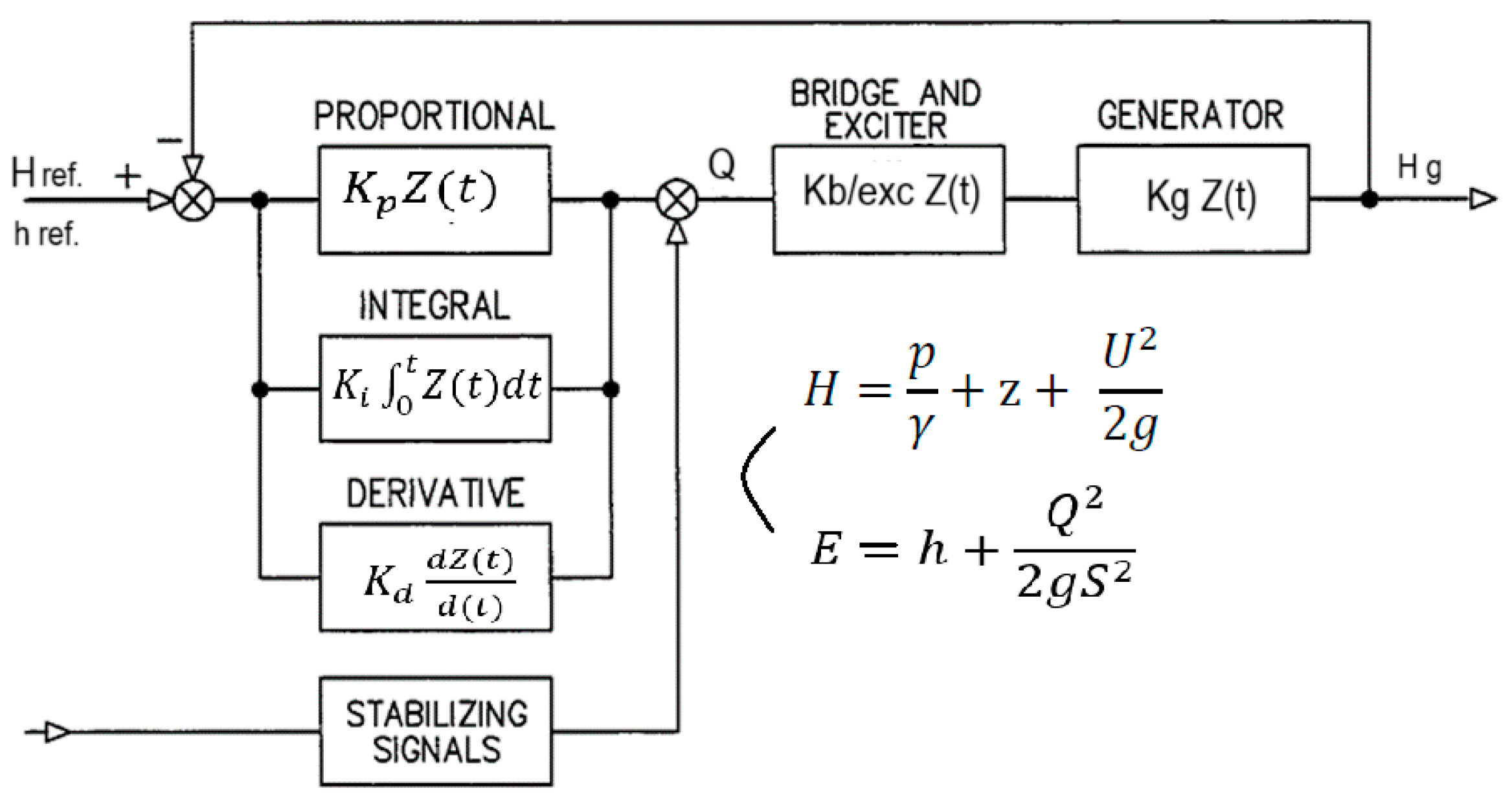
2.2.11. Water Level Control (PID Regulator)

The closing of a valve or gate can trigger a hydraulic bore that spreads upstream. This phenomenon can create a series of surge waves that lead to an increase in flow velocity and water depth, especially in the upstream sections. In canals, the lateral walls can overflow if they are not high enough. To avoid flooding, suitable side walls must be designed, which can increase considerably the costs.

When the hydropower is shut down, a positive surge is observed that starts with a wave surge which can turn into a breaking surge [10,11]:

Along a canal, it verifies four stages of the waves:

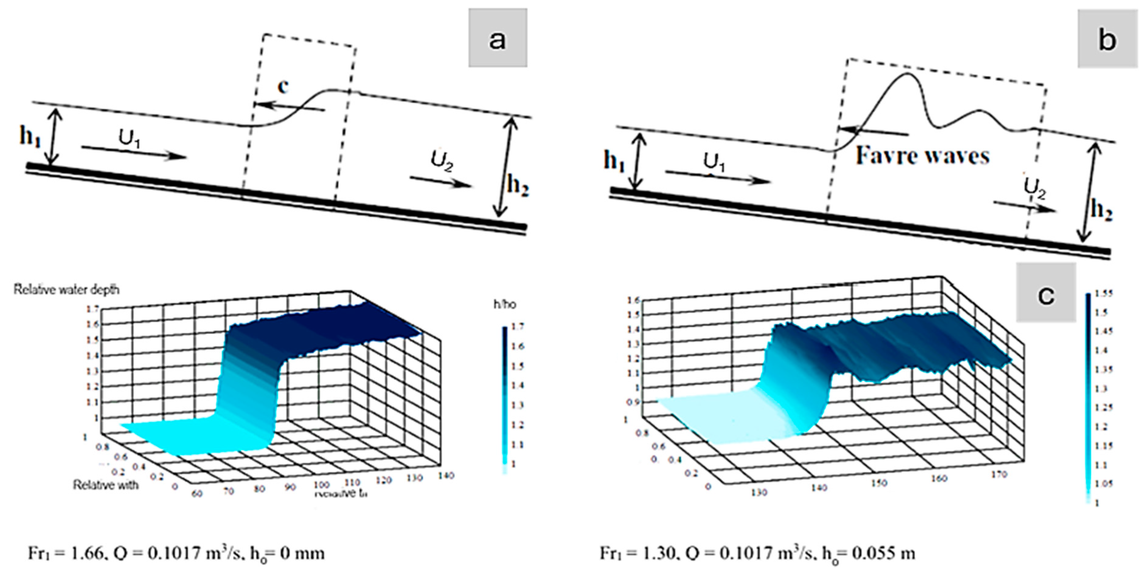
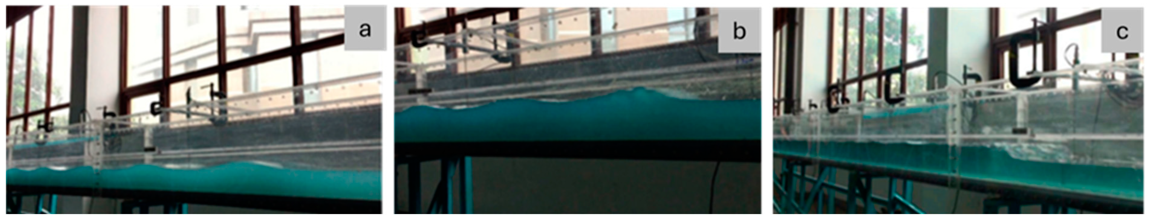
• Stage 1: the front of the shaft is fairly smooth;
• Stage 2: the wave head becomes rough and forms some waves on the surface (Figure 11a).
• Stage 3: flatter waves are observed, and the amplitude of the wave is shown to decrease (Figure 11b).
• Stage 4: the front of the wave is practically vertical, and these waves are called breaking tidal waves (Figure 11c).

The consequences of hydraulic drilling can be mitigated by installing a water level regulator in the forebay. This device controls the closing of the turbine valve or the lock gates to raise or lower the water level in the forebay. By controlling the closing of the turbine shutter, it creates waves of lower amplitude, which has considerable advantages to reduce the height of the side walls. On the other hand, the regulator allows for the damping of the waves over time.

In a viscous model, the damping force (F_d) is proportional to the velocity and has an opposite direction to the motion (Equation (36)).

$${\mathrm{F}}_{\mathrm{d}}=-\mathrm{c}\stackrel{·}{\mathrm{Z}}\left(\mathrm{t}\right)$$

(36)

where:

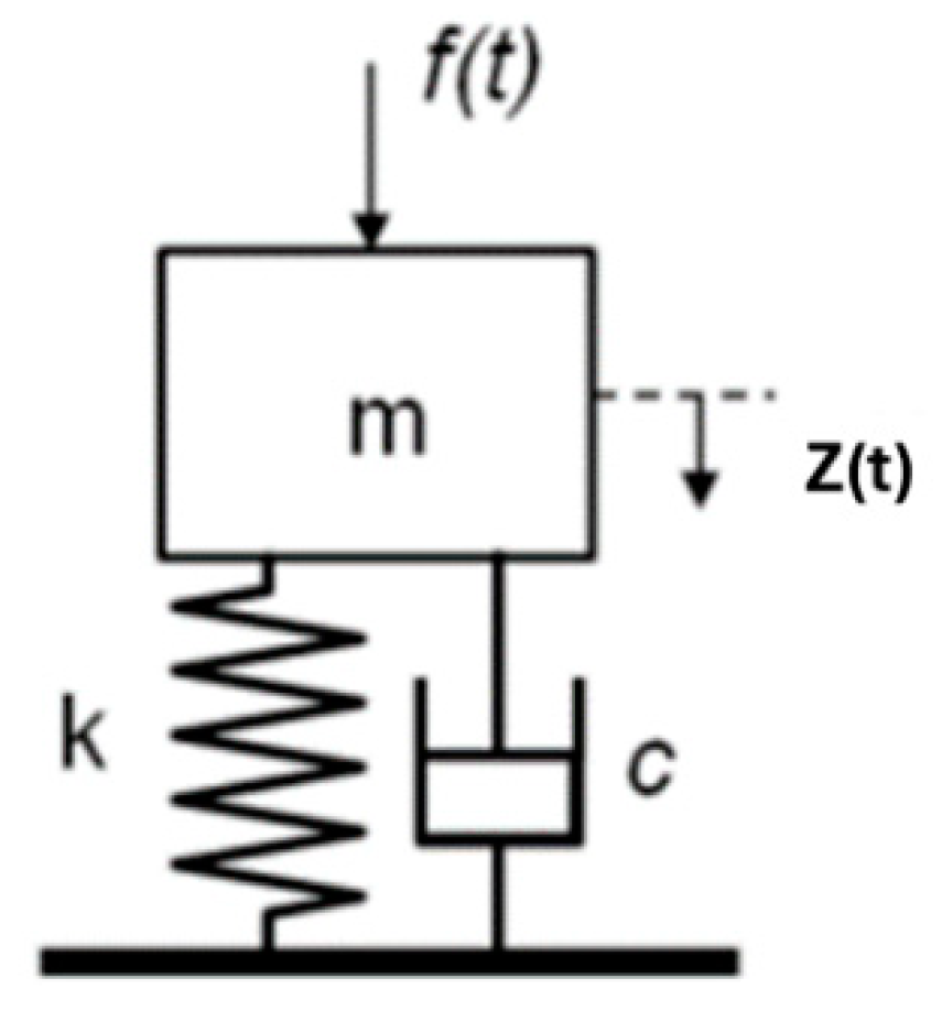
• c is the damping coefficient;
• $\stackrel{·}{\mathrm{Z}}$(t) is the velocity of movement of a mass to a fixed point.

The control is based on the equation of motion of the damped free oscillation developed by Isaac Newton (Equation (37)), which occurs in a mass-spring-damper model [4] (Figure 12).

$$\mathrm{m}\ddot{\mathrm{Z}}\left(\mathrm{t}\right)+\mathrm{c}\stackrel{·}{\mathrm{Z}}\left(\mathrm{t}\right)+\mathrm{kZ}\left(\mathrm{t}\right)=0$$

(37)

where k is the spring constant, and Z(t) is variation in the water depth provoked by surge waves with a periodic and non-periodic oscillatory motion, and finally $\ddot{\mathrm{Z}}$(t) is the acceleration.

The solution of Equation (37), with the displacement as a function of time, can then be obtained via Equation (38):

$$\mathrm{Z}\left(\mathrm{t}\right)={\mathrm{Ae}}^{\mathrm{st}}$$

(38)

where A and s are constants. The function s is defined by Equation (39).

$${\mathrm{s}}_{1,2}=-{\displaystyle \frac{\mathrm{c}}{2\mathrm{m}}}\pm \sqrt{{\left({\displaystyle \frac{\mathrm{c}}{2\mathrm{m}}}\right)}^2-\left({\displaystyle \frac{\mathrm{k}}{\mathrm{m}}}\right)}$$

(39)

Considering that the angular velocity is equal to $\mathrm{w}=\sqrt{{\displaystyle \frac{\mathrm{k}}{\mathrm{m}}}}$, the critical damping coefficient, c_c, becomes the second term of Equation (39) and is equal to 0 and can be calculated using Equation (40).

$${\mathrm{c}}_{\mathrm{c}}=2\mathrm{wm}$$

(40)

The viscous damping ratio coefficient, $\xi$, is obtained by dividing the damping coefficient with the critical damped (Equation (41)).

$$\mathsf{\xi }={\displaystyle \frac{\mathrm{c}}{{\mathrm{c}}_{\mathrm{c}}}}={\displaystyle \frac{\mathrm{c}}{2\mathrm{wm}}}$$

(41)

Each system can be classified based on its phase into three different groups:

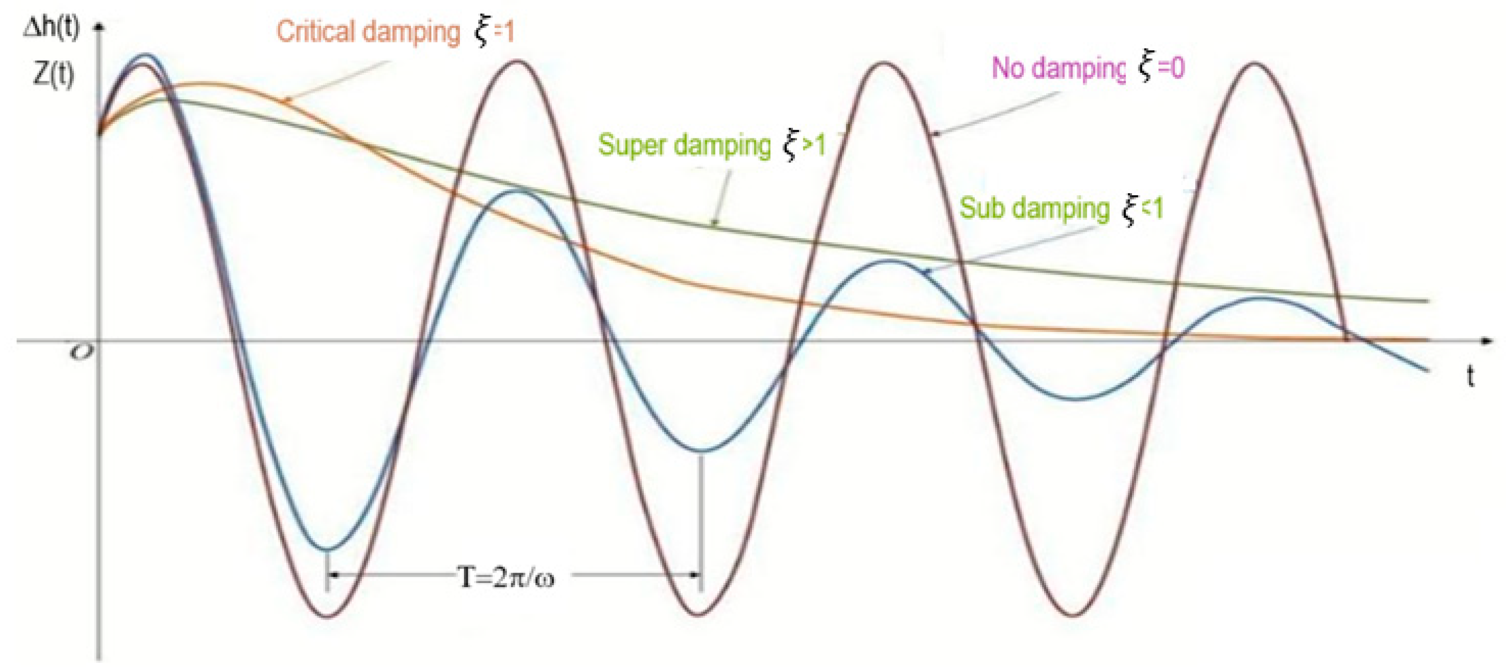
• if ξ < 1, the system is called underdamped;
• if ξ = 1 the system is called critically damped;
• if ξ > 1, the system is called overdamped.

Figure 13 shows the behavior of the systems for each of these groups.

Based on the calculation of the damping ratio, it is possible to rewrite Equation (42).

$${\mathrm{S}}_{1,2}=-\mathsf{\xi }\mathrm{w}\pm \mathrm{i}\sqrt{1-{\mathsf{\xi }}^2}\mathrm{w}$$

(42)

where i is the imaginary unit.

A simple harmonic motion (SHM) is a periodic motion that occurs in conservative systems. In this system, when a simple body is perturbed, it returns to the equilibrium position because no dissipative forces are acting on the body. The change in position as a function of time is given by Equation (43), where $\varphi$ is the phase constant:

$$\mathrm{Z}\left(\mathrm{t}\right)=\mathrm{Acos}\left(\mathrm{wt}+\varphi \right)$$

(43)

There is no conservative system. In this way, there is a loss of energy in all systems, which decreases exponentially over time. Taking this dissipation into account, the change in position can be rewritten as a function of time (Equation (44)):

$$\mathrm{Z}\left(\mathrm{t}\right)={\mathrm{Ae}}^{-\mathsf{\xi }\mathrm{wt}}\cos \left(\mathrm{wt}+\varphi \right)$$

(44)

The regulator is controlled based on a P.I.D. solution [3,4] (Proportional, Integral, and Derivative) (Figure 13). Combining Equations (37) and (44), the P.I.D. equation (Equation (45)) is obtained.

$$\Delta \mathrm{h}\left(\mathrm{t}\right)={\mathrm{K}}_{\mathrm{p}}\mathrm{Z}\left(\mathrm{t}\right)+{\mathrm{K}}_{\mathrm{i}}{\int }_0^{\mathrm{t}}\mathrm{Z}\left(\mathrm{t}\right)\mathrm{dt}+{\mathrm{K}}_{\mathrm{d}}{\displaystyle \frac{\mathrm{dZ}\left(\mathrm{t}\right)}{\mathrm{d}\left(\mathrm{t}\right)}}$$

(45)

where Δh(t) represents the change in surge waves above the output level in the forebay per unit of time in a specific section. K_p, K_i, and K_d are the proportional, integral, and derivative coefficients of the controller, respectively. These coefficients make it possible to reduce the amplitude of the oscillations when the hydraulic bore occurs.

Figure 14 shows that the water depth of the surge waves, which are triggered by the turbine shutdown, decreases significantly when a PID controller is installed. On the other hand, the free surface with a PID governor is more undulating and degrades over time.

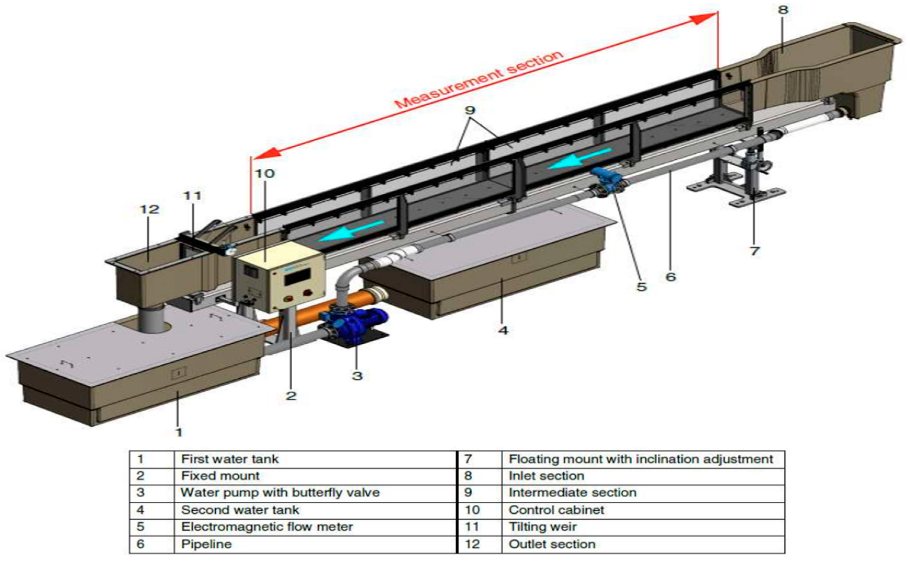
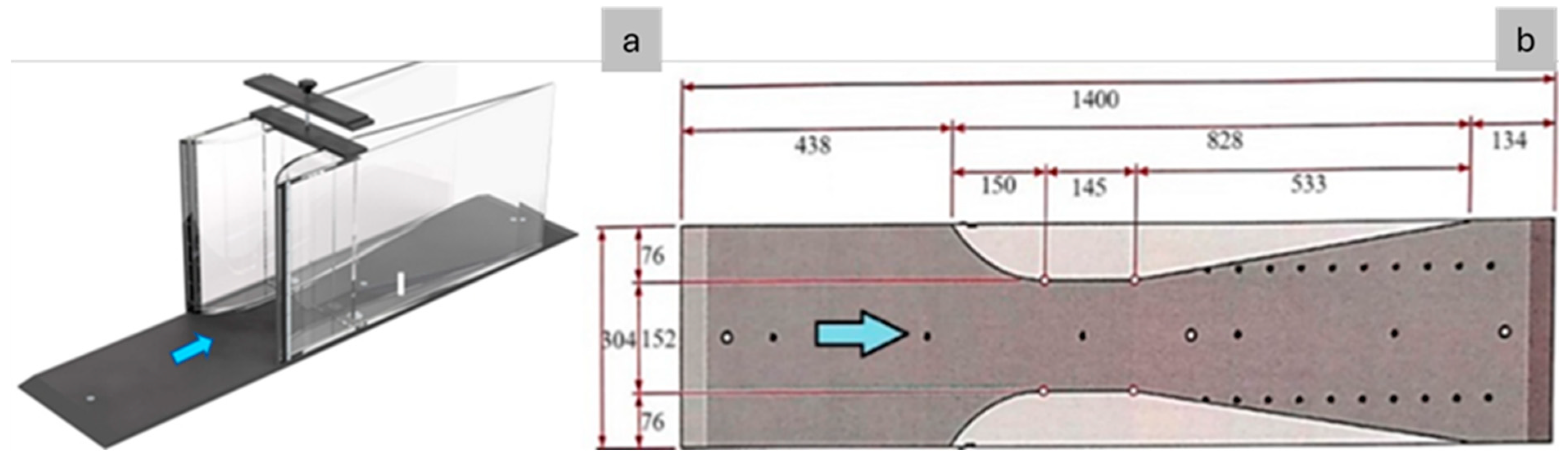
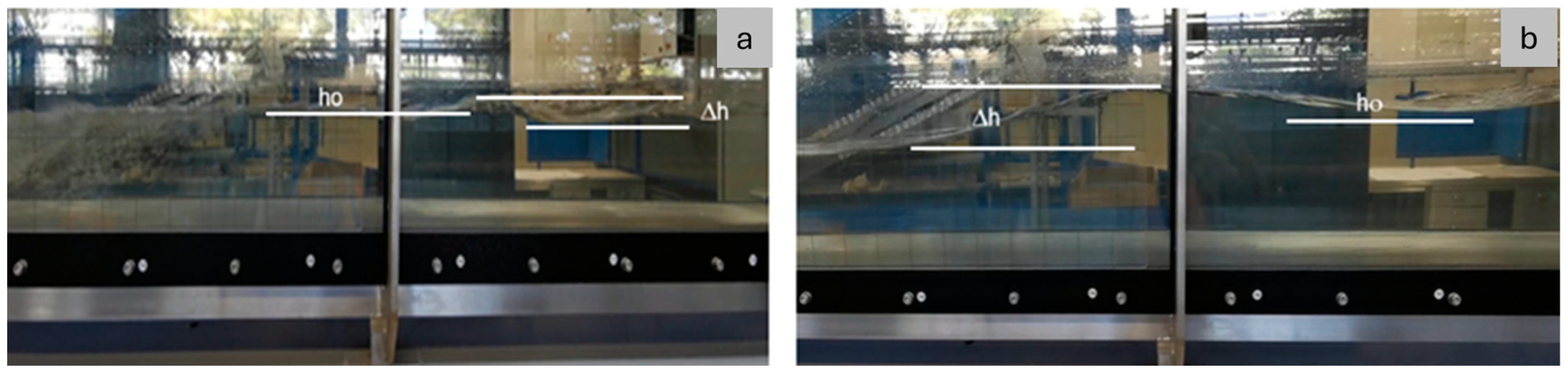
2.3. Experimental Tests and Case Study

Lab Set-Up Description

The experimental tests were carried out in the Hydraulics and Water Resources Laboratory of the Department of Civil Engineering, Architecture, and Environment (DECivil) of the Instituto Superior Técnico (IST). In these tests, a variable slope channel was used, as shown in Figure 15. In this channel, the water is stored in two reservoirs, (1) and (4), and then pumped into another reservoir (8), which has a surface stabilizer. The flow takes place on a free surface over the entire length of the channel. At the end of the channel, there is a gate that controls the water depth downstream. When the river has passed the gates, it flows back into the reservoir (1).

To measure the flow rate, a flow meter (5) is installed downstream of the pump. The water depth of the flow can be measured in two different ways: with a hydrometer attached to the canal walls that can be moved along the length and width of the canal or with a series of piezometers installed at 25 cm intervals at the bottom of the canal. A scale attached to the left wall of the channel in the direction of flow allows the measurement of the sections where the measurements take place. The dimensions and characteristics of the channel are given in

Table 1. Canal characteristics.

Length (m)	5	Wall Thickness (m)	0.008
Width (m)	0.309	K (m1/3s−1)	100
Height (m)	0.45	Slope (%)	−0.5 to 2.5

, where K represents the Strickler coefficient.

It can install some accessories in the channel to simulate certain hydraulic conditions. Figure 16 shows a longitudinal scheme of the channel when a constriction is placed in the upstream section.

Figure 17a,b show the constriction used and its dimensions (in mm).

Levadas is a canal system that is more than 3800 km long (Figure 18) on the island of Madeira, which was built in the 16th century. The canal was used to transport water from the wetter regions of the island to the dry areas used for agriculture. Nowadays, it is also used to transport water for water consumption and to generate electricity.

This study includes the evaluation of the behavior of the water when it enters the Covão tunnel and then passes through the forebay to the penstock (Figure 19) that connects Covão to Socorridos.

3. Discussion of Obtained Results

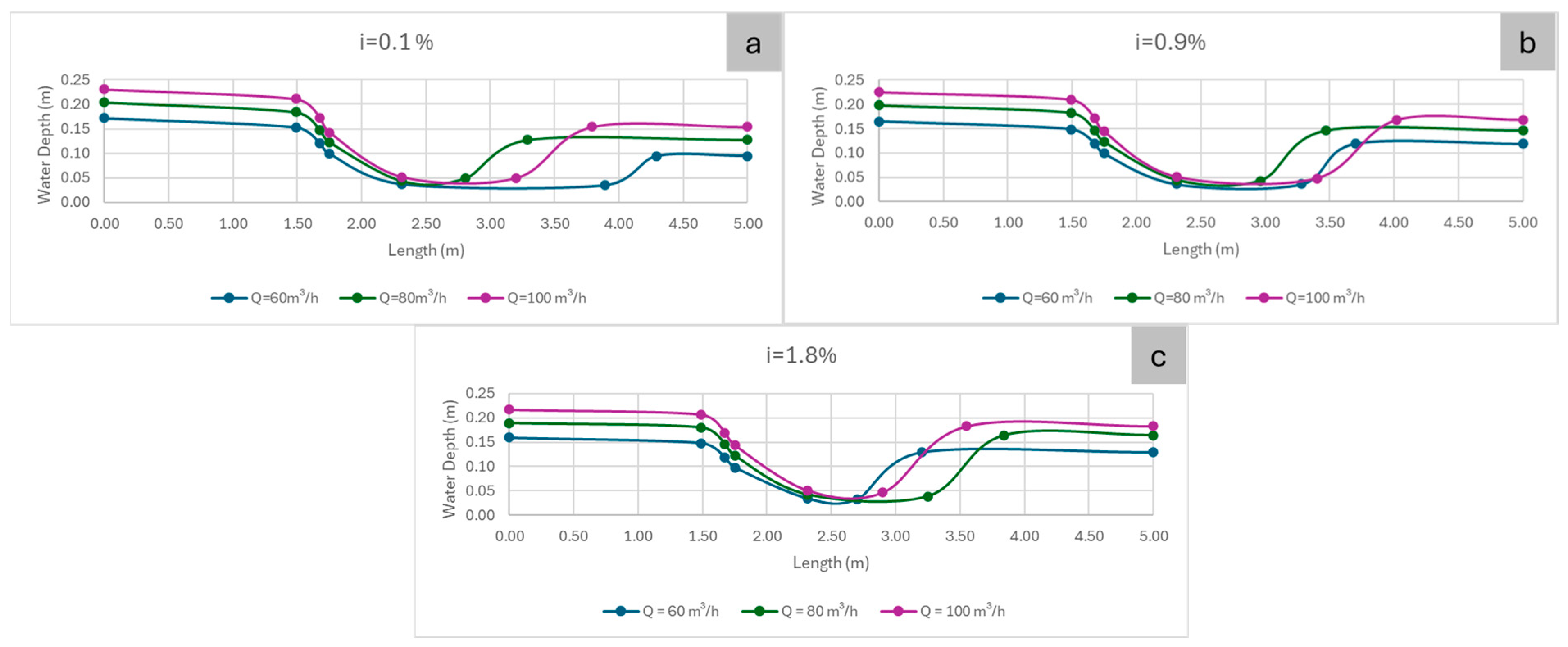
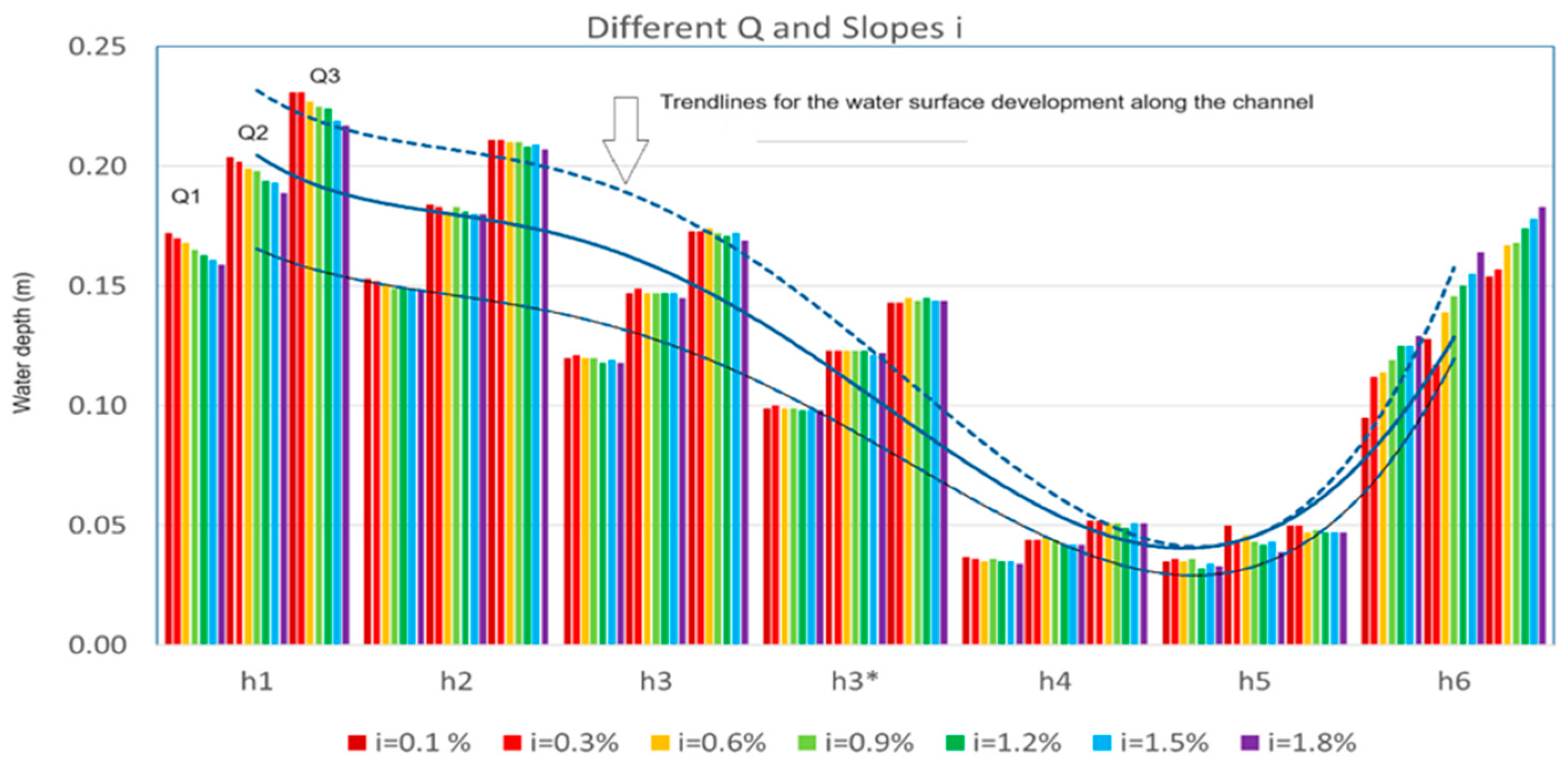
3.1. Gradually Varied Flow

In order to simulate the water entering the Covão tunnel and the hydraulic bore that can form in the event of a sudden flow modification, tests were carried out with different flow rates (60 to 100 m³/h), each with seven different slopes (0.1, 0.3, 0.6, 0.9, 1.2, 1.5, and 1.8%). However, in some figures, only three flow rates (60, 80, and 100 m³/h) and three slopes (0.1, 0.9, and 1.8%), were considered, because the other intermediate values do not add significant information. The critical slope (i_c) associated with each flow rate is shown in

Table 2. Critical slopes for each flow rate.

Q (m3/h)	ic
60	75%
70	64%
80	56%
90	50%
100	45%

.

The slopes considered are always below the critical slope, which means the uniform flow is greater than the critical one, and the flow is described as subcritical. The backwater curves for different Froude numbers and the scheme of the hydraulic jump at a mild slope (i.e., below the critical slope) are shown in Figure 20a,b.

The uniform (h_u) and critical (h_c) water depths are represented and shown in Figure 21 for each type of flow velocity and slope.

In Figure 21, both the uniform and the critical water depth increase with the flow rate. At the same flow rate, the uniform water depth decreases as the slope increases. However, the critical water depth does not depend on the value of the slope.

Figure 22 shows the relationship between the curves of E/E_c and $\mathbb{M}/{\mathbb{M}}_{\mathrm{c}}$ as a function of the non-dimensional water depth (h/h_c).

An important aspect is that the minimum specific energy and the minimum total momentum occur at the critical depth. The difference between points 5 and 6 in the curve $\mathbb{M}/{\mathbb{M}}_{\mathrm{c}}$ = f(h/h_c) shows that the total momentum keeps constant in the hydraulic jump, which means that the associated resultant forces can be easily estimated and are the same.

However, observing the same points, but in the curve E/E_c, it is possible to see that the head loss can be estimated for the hydraulic jump and compared with Equation (25). At the constriction, as expected according to the principle of energy conservation, points 2 and 4 on the dimensionless energy curve coincide, being the critical energy of the narrowest cross-section.

The water depth as a function of the flow rate per unit width at the constriction can be determined using Equation (12). Figure 23 shows the theoretical curves with the same specific energy derived for each flow rate per unit width and a comparison with the results obtained experimentally. Both subcritical and supercritical flows are identified above and below the maximum flow transport capacity, respectively, reflecting the critical conditions.

The experimental results agree with theoretical curves. However, as the flow rate per unit width increases, the experimental results deviate slightly from the results predicted by the curves due to additional turbulence.

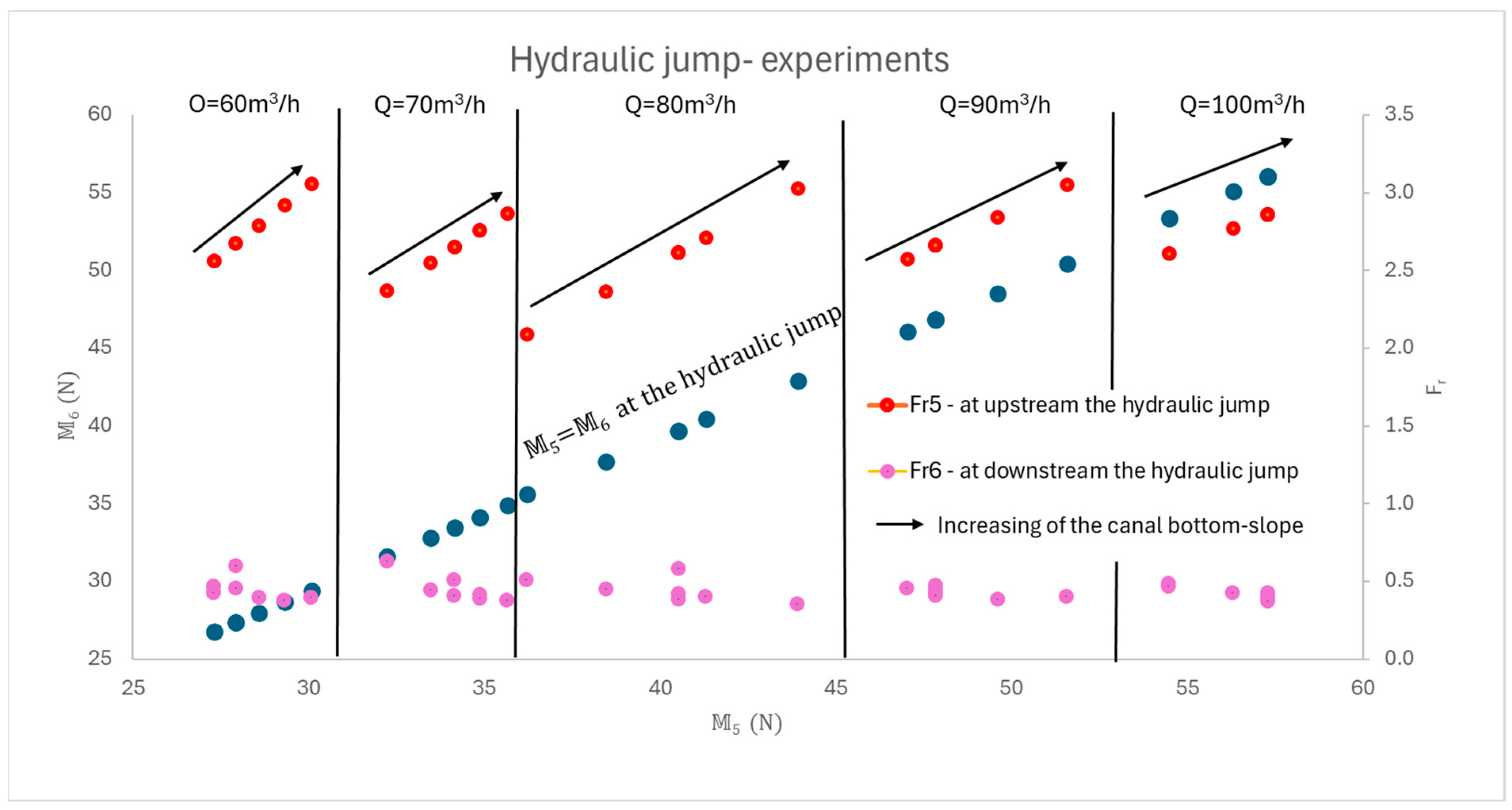
3.2. Rapidly Varied Flow

The hydraulic jump is illustrated in Figure 24a–c, which show the profile of the free surface for each slope with different flow rates. The water depth tends to increase with subcritical and supercritical flow as the flow rate increases. Another important issue is that the hydraulic jump tends to increase for the same flow rate when the slope increases and the length for Q = 100 m³/h varies from 0.55 to 1.00 m when the slope “I” varies from 0.1% to 1.8%. In these cases (Figure 25), the variation in the slope also influences the water depth upstream and downstream.

In the upstream section (1) in Figure 16, considerable differences in water depths between flow rates can be observed during the subcritical flow. However, when the flow changes to a supercritical state (sections (4) and (5)—Figure 16), the water depth varies less at the different flow rates. It is worthwhile to emphasize that the water depth in the subcritical flow is about two to four times higher than in the supercritical flow, depending on the flow rate value. This indicates that during a hydraulic jump with additional bore, the water depth increases sharply. If the side walls of the channel are not designed for this phenomenon, they are likely to be flooded. The water-free surface in a channel can vary greatly depending on the singularities and boundary conditions [25,26,27].

Figure 26a–c show the differences in the water depths and flow vorticity as well as the turbulence with emulsified air with dissipation energy at the hydraulic jump.

The length of the hydraulic jump can be determined using different estimations, which are presented in [25]. In order to analyze the differences between these equations and to determine the one that best fits the experimental determined results, two graphs were created, which are shown in Figure 27a,b.

Figure 28 shows the Peterka curve does not fit the experimental results efficiently, as it is mainly used for higher flow rates. In contrast, the curves presented by [25] agree better with the laboratory tests as they are suitable for low upstream heights of the hydraulic jump (h₅). Some experimental points agree well with the results of the Kumin curve.

Figure 28 shows the relationship between the total momentum and the Froude number in the upstream and downstream sections of the hydraulic jump. Analyzing the results, the total momentum increases when the flow rate and the slope increase. On the other hand, the Froude number in the upstream section of the hydraulic jump increases with the increase in the slope. The flow rate does not have much influence on the value of the Froude number, since, for the same slope, when it increases, the water level also increases, and it is not possible to establish a relationship between the flow rate and the Froude number.

For example, considering an average flow value of 80 m³/h, the head loss in the hydraulic jump is estimated as follows using the E/E_c curve and the empirical formulation:

Experimental value based on Figure 27: ΔE_r = 0.04 m;

Empirical (Equation (25)): $\Delta {\mathrm{E}}_{\mathrm{r}}={\displaystyle \frac{{\left({\mathrm{U}}_1-{\mathrm{U}}_2\right)}^2}{2\mathrm{g}}}-{\displaystyle \frac{{\left({\mathrm{h}}_2-{\mathrm{h}}_1\right)}^2}{{\mathrm{h}}_2}}$ = 0.117 − 0.077 = 0.0395 m.

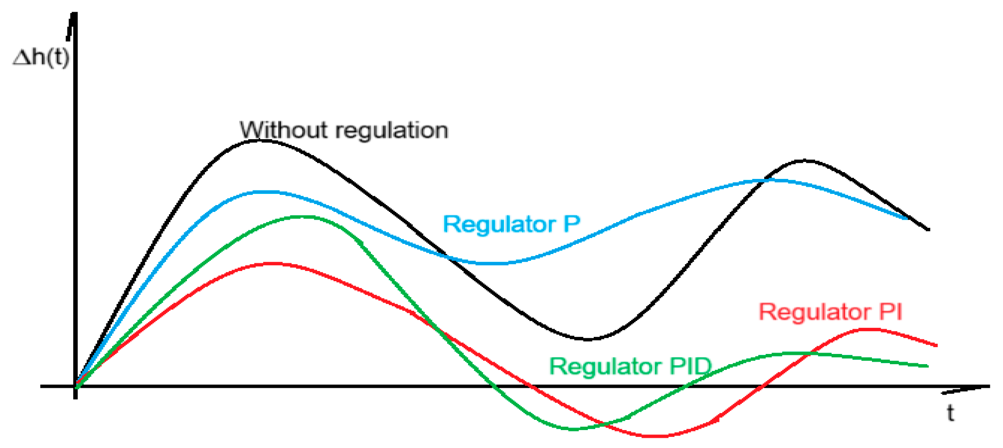
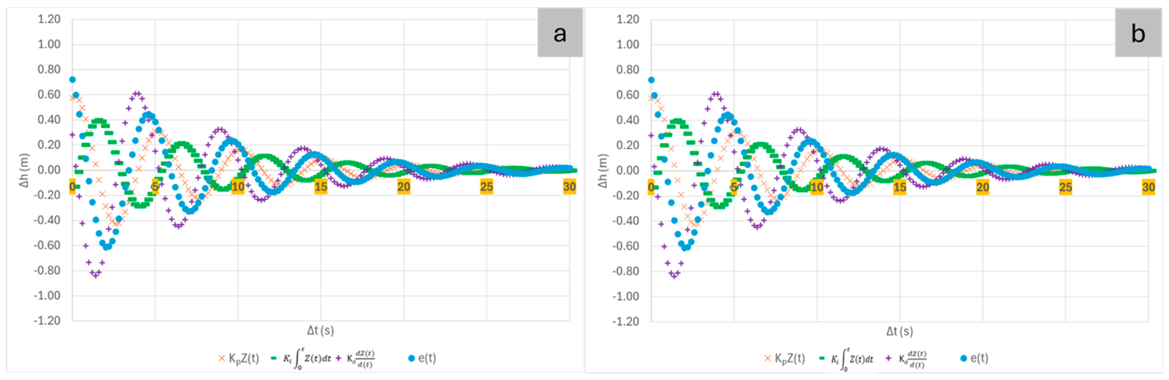
3.3. Simulation of a PID Regulator

3.3.1. Parameters and Operating Scheme

Two different methods were used to analyze the fluctuations in water surface in the forebay. In both methods, the following values were considered for each parameter (

Table 3. Parameters for the PID regulator.

A (m)	T (s)	Kp	Ki	Kd	ξ	w (rad/s)	ϕ	dt (s)
2	5	0.3	0.3	0.4	0.1 or other	1.257	6	0.2

Note: A = maximum amplitude of the wave, T = wave period, and dt = integration time instant.

).

Starting from the simple harmonic motion (SHM) that characterizes the water level oscillation in a water intake or an open channel or a forebay, the water level regulation can be based on a PID (Proportional, Integral and Derivative) controller to provide stable and efficient control to avoid overflow. As a reminder, the movement can be characterized by Equations (46) and (47):

$$\mathrm{Z}\left(\mathrm{t}\right)={\mathrm{Ae}}^{-\mathsf{\xi }\mathrm{wt}}\cos \left(\mathrm{wt}+\varphi \right)$$

(46)

$$\mathsf{\Delta }\mathrm{h}\left(\mathrm{t}\right)={\mathrm{K}}_{\mathrm{p}}\mathrm{Z}\left(\mathrm{t}\right)+{\mathrm{K}}_{\mathrm{i}}{{\displaystyle \int }}_0^{\mathrm{t}}\mathrm{Z}\left(\mathrm{t}\right)\mathrm{dt}+{\mathrm{K}}_{\mathrm{d}}{\displaystyle \frac{\mathrm{dZ}\left(\mathrm{t}\right)}{\mathrm{d}\left(\mathrm{t}\right)}}$$

(47)

The PID modeling is represented in Figure 29.

3.3.2. Formulations for Water Level Regulation Without Damping Effect

Without any damping effect, the water level fluctuates continuously over time without any dissipation. The movement is described by the following Equations (48)–(50) and Figure 30.

$$\mathrm{Z}\left(\mathrm{t}\right)=\mathrm{Acos}\left(\mathrm{wt}+\varphi \right)$$

(48)

$${\int }_0^{\mathrm{t}}\mathrm{Z}\left(\mathrm{t}\right)\mathrm{dt}=\left({\displaystyle \frac{\mathrm{A}}{\mathrm{w}}}\right)\sin \left(\mathrm{wt}+\varphi \right)$$

(49)

$${\displaystyle \frac{\mathrm{dZ}\left(\mathrm{t}\right)}{\mathrm{dt}}}=-\mathrm{wAsin}\left(\mathrm{wt}+\varphi \right)$$

(50)

Hence, the harmonic model shows uncontrolled regulation after the onset of the flow disturbance, which makes the restart of the hydropower or pumping system very unstable and difficult.k_D

3.3.3. Regulation with Dissipative Effect

A first approach considers the SHM with the dissipation effect, $e^{-\xi wt},$ applied after the definition of the characteristic equations. The representation of each term and the total variation in each time are represented in Equations (51) and (52) and Figure 31.

$${\int }_0^{\mathrm{t}}\mathrm{Z}\left(\mathrm{t}\right)\mathrm{dt}=\left({\displaystyle \frac{\mathrm{A}}{\mathrm{w}}}\right){\mathrm{e}}^{-\mathsf{\xi }\mathrm{wt}}\sin \left(\mathrm{wt}+\varphi \right)$$

(51)

with

$${\displaystyle \frac{\mathrm{dZ}\left(\mathrm{t}\right)}{\mathrm{dt}}}=-{\mathrm{wAe}}^{-\mathsf{\xi }\mathrm{wt}}\sin \left(\mathrm{wt}+\varphi \right)$$

(52)

Figure 29 shows the water surface of the surge waves decreases as induced by the PID actuation. This is very beneficial because the channel walls can have a correct height, with safe and more economical building. On the other hand, it gives confidence in controlling the probability of flooding. Another important issue is that the waves are attenuated over time, and depending on the characteristic parameters of the regulator, a decrease in the free surface to the initial state can be observed in less than a few seconds. After this period, the water surface attains to the initial conditions.

In the second approach, mathematical operators were applied to the dissipation term. ${\mathrm{e}}^{-\mathsf{\xi }\mathrm{wt}}$ in the functions ${\int }_0^{\mathrm{t}}\mathrm{Z}\left(\mathrm{t}\right)\mathrm{dt}$ and ${\displaystyle \frac{\mathrm{dZ}\left(\mathrm{t}\right)}{\mathrm{dt}}}$ (Equations (53) and (54)).

$${\int }_0^{\mathrm{t}}\mathrm{Z}\left(\mathrm{t}\right)={\mathrm{Ae}}^{-\mathsf{\xi }\mathrm{wt}}{\displaystyle \frac{{\mathrm{e}}^{-\mathsf{\xi }\mathrm{wt}}}{\mathrm{w}({\mathsf{\xi }}^2+1)}}\left(\mathsf{\xi }\cos \left(\mathrm{wt}+\varphi \right)-\sin \left(\mathrm{wt}+\varphi \right)\right)$$

(53)

$${\displaystyle \frac{\mathrm{dZ}\left(\mathrm{t}\right)}{\mathrm{dt}}}=-{\mathrm{Awe}}^{-\mathsf{\xi }\mathrm{wt}}\left(\mathsf{\xi }\cos \left(\mathrm{wt}+\varphi \right)+\sin \left(\mathrm{wt}+\varphi \right)\right)$$

(54)

Figure 31 shows the variation in water depth for each component using both approaches, where it is noticeable that the results are equivalent for these system characteristics. For both cases, it was considered a damping ratio equal to 0.1.

Analyzing Figure 31, the water depth variation over time is the same in both approaches. This concludes that the integration and the derivation of the damping term $e^{-\xi \mathrm{wt}}$ does not influence the variation in the surface water level for each component of the PID for this analysed system.

In order to observe the hydraulic bore induced by a flow variation, two tests were carried out: the first with a flow rate of 60 m³/h and the second with a flow rate of 100 m³/h. In these two tests, the slope is 1.8%. Higher oscillation was found with higher flow rate.

Figure 32 shows the surge waves for about Δh~20 to 40% between the positive and negative fluctuations for Q = 60 and 100 m³/h, becoming more pronounced at the same slope when the flow rate increases.

3.3.4. Sensitivity Analysis of the Damping Effect

To study the influence of the damping effect in the propagation of the negative surge wave under a PID control system, a sensitivity analysis was developed with different values adopted for the damping ratio coefficient, ξ (Figure 33a–c).

Increasing the damping ratio reduces the amplitude and phase duration of the water surface oscillations in the forebay of the Levadas, from about 25 s to 5 s total duration, thus avoiding the resonance effect with reflection waves and allowing the power stations to restart more efficiently with less loss of time. At high values for the damping coefficient, the change in water surface takes only a few seconds (less than 5 s for the scaled case study) and then returns to the initial static level. During the design project, the characteristics and limitations of the system should be taken into account when defining the operating constraints.

4. Conclusions

In this research study, a mathematical modelling and an experimental analysis were conducted to improve the hydrodynamic flow model hazards that can destabilize the channel flow conditions due to constrictions, gate obstructions, and hydroelectric power plant/pump start-up or shutdown.

All the mathematical formulations based on the hydraulic concepts of government equations based on the continuity, flow energy, and momentum were defined to model and analyze the flow behavior in free surface flow components of a long and mixed hydraulic circuit.

A forebay at the downstream end of a tunnel or canal is analyzed to ensure adequate conditions for the installation of the penstock water intake and associated equipment (e.g., trash racks, gates, sluices, and weirs) while maintaining minimum flooding criteria, limiting flow fluctuations along the canal due to variations in turbine discharge, and providing a regulating function to meet the temporary needs of the turbines regardless of the flow regime.

The profile of water depth along an open channel changing with flow conditions, from steady flow to gradually and rapidly changing flow (with clearly curved streamlines and multidimensional) was analyzed. Constriction cross-sections and hydraulic jumps as flow boundary conditions were investigated in detail with experimental tests for a flow range between 60 and 100 m³/h. The specific energy in the constriction cross-section and the total momentum in the hydraulic jump were used to derive the formulations used to justify the channel obstructions, such as cross-section and water profile variations affecting the open channel behavior with additional surge effects. The constriction was used to study the passage from the water intake of the Levadas channel to the Covão tunnel and the forebay. In these situations, the specific energy remains constant. The water passes from the subcritical flow in the upstream section to the supercritical flow in the downstream section, increasing the velocity in the penstock and keeping the critical specific energy constant. The best estimates for the length of the hydraulic jumps come from Kumin and Mundo-Molina, with values between 0.55 and 1.00 m, and the head losses in the hydraulic jump match the experiments with a value of around 0.04 m, both under laboratory conditions.

A sudden interruption in turbine operation can trigger a hydraulic bore that propagates upstream in the forebay or channel. These events lead to secondary oscillation waves that may cause the canal walls to overflow. On the other hand, if the flow rate in the turbine is increased, the supply capacity of the channel may be exceeded, and air may enter, which must be avoided. A mathematical formulation of a PID controller is developed and analyzed to control and reduce positive and negative waves (such as bores) and upstream wave propagation, which can jeopardize the safety of the hydraulic structure of the lateral wall overflow channel. Waves triggered by the rapid closing of a gate or the shutdown of a powerhouse cause the water level to rise by about 20-40%. Using a PID controller after a sensitivity analysis, the waves could be reduced to 0.8 m, and the dissipation can be achieved in less than 20 s.

References

- Safdar, I.; Sultan, S.; Raza, H.A.; Umer, M.; Ali, M. Empirical analysis of turbine and generator effciency of a Pico hydro system. Sustain. Energy Technol. Assess. 2020, 37, 100605. [Google Scholar] [CrossRef]
- Safarian, S.; Unnþórsson, R.; Ritcher, C. A review of biomass gasification modelling. Renew. Sustain. Energy Rev. 2019, 110, 378–391. [Google Scholar] [CrossRef]
- Ramos, H. Guidelines for Design of Small Hydropower Plants; WREAN (Western Regional Energy Agency and Network) and DED (Department of Economic Development-Energy Division): Belfast, UK, 2000; pp. 153–154. [Google Scholar]
- Masotti, D. Comparison of Methods for Determining Structural Damping Through Frequency Response Function Curve-Fitting Techniques; Universidade Federal de Santa Catarina: Florianopolis, Brazil, 2013; pp. 46–49, 65–66. [Google Scholar]
- Liggett, J.A. Fluid Mechanics; McGraw-Hill: New York, NY, USA, 1994. [Google Scholar]
- Lighthill, J. Waves in Fluids; Cambridge University Press: Cambridge, UK, 1978; p. 504. [Google Scholar]
- Wanoschek, R.; Hager, W.H. Hydraulic jump in trapezoidal channel. J. Hydraul. Res. 1989, 27, 429–446. [Google Scholar] [CrossRef]
- Chanson, H. Momentum considerations in hydraulic jumps and bores. J. Irrig. Drain. Eng. 2012, 138, 382–385. [Google Scholar] [CrossRef]
- Kiri, U.; Leng, X.; Chanson, H. Positive Surge Propagation in a Non-Rectangular Asymmetrical Channel; Hydraulic Model Report No. CH110/18; School of Civil Engineering, The University of Queensland: Brisbane, Australia, 2018; p. 159. [Google Scholar]
- Treske, A. Undular bores (favre-waves) in open channels—Experimental studies. J. Hydraul. Res. 1994, 32, 355–370. [Google Scholar] [CrossRef]
- Zheng, F.; Li, Y.; Xuan, G.; Li, Z.; Zhu, L. Characteristics of positive surges in a rectangular channel. Water 2018, 10, 1473. [Google Scholar] [CrossRef]
- Leng, X.; Chanson, H. Coupling between free-surface fluctuations, velocity fluctuations and turbulent Reynolds stresses during the upstream propagation of positive surges, bores and compression waves. Environ. Fluid Mech. 2016, 16, 695–719. [Google Scholar] [CrossRef]
- Shi, J.; Tong, C.; Yan, Y.; Luo, X. Influence of varying shape and depth on the generation of tidal bores. Environ. Earth Sci. 2014, 72, 2489–2496. [Google Scholar] [CrossRef]
- Kiri, U.; Leng, X.; Chanson, H. Positive surge propagating in an asymmetrical canal. J. Hydro-Environ. Res. 2020, 31, 41–47. [Google Scholar] [CrossRef]
- Musa, R.; Triffandy, M.W.; Rusaldy, A. Application of Specific Energy in Open Channels to Various Forms of Channel Constriction. WSEAS Trans. Appl. Theor. Mech. 2022, 17, 39–46. [Google Scholar] [CrossRef]
- Harianja, J.A.; Gunawan, S. Overview of Specific Energy Due to Constriction of Open Channels, 1st ed.; Scientific Magazine; UKRIM: Yogyakarta, Indonesia, 2007; pp. 30–46. [Google Scholar]
- Musa, R.; Rusaldy, R.A. Analysis of Changes in the Effect Flow Rate on the Open Channel. In Proceedings of the International Seminar of Science and Applied Technology (ISSAT 2020), Virtual, 24 November 2020. [Google Scholar]
- Cheng, Y.; Song, Y.; Liu, C.; Wang, W.; Hu, X. Numerical Simulation Research on the Diversion Characteristics of a Trapezoidal Channel. Water 2022, 14, 2706. [Google Scholar] [CrossRef]
- Li, T.; Zou, J.; Qu, S.J.; Liu, Z.; Ren, Z.H.; Tian, W.J. Local head loss of 90° lateral diversion from open channels of different cross-sectional shapes. J. Hydroelectr. Eng. 2017, 36, 30–37. [Google Scholar]
- Hadian, S.; Afzalimehr, H.; Ahmad, S. Effects of Channel Width Variations on Turbulent Flow Structures in the Presence of Three-Dimensional Pool-Riffle. Sustainability 2023, 15, 7829. [Google Scholar] [CrossRef]
- Wan, Z.; Li, Y.; Wang, X.; An, J.; Dong, B.; Liao, Y. Influence of Unsteady Flow Induced by a Large-Scale Hydropower Station on the Water Level Fluctuation of Multi-Approach Channels: A Case Study of the Three Gorges Project, China. Water 2020, 12, 2922. [Google Scholar] [CrossRef]
- Li, W.; Wang, D.; Yang, S.; Yang, W. Three Gorges project: Benefits and challenges for shipping development in the upper Yangtze river. Int. J. Water Resour. Dev. 2020, 37, 758–771. [Google Scholar] [CrossRef]
- Jia, T.; Qin, H.; Yan, D.; Zhang, Z.; Liu, B.; Li, C.; Wang, J.; Zhou, J. Short-term multi-objective optimal operation of reservoirs to maximize the benefits of hydropower and navigation. Water 2019, 11, 1272. [Google Scholar] [CrossRef]
- Pinheiro, A. Hydraulic II, Chapter 1, Free Surface Flows. Version 2021. IST. (In Portuguese)
- White, F.M. Fluid Mechanics, 7th ed.; Mcgraw-Hill Series in Mechanical Engineering; McGraw-Hill: New York, NY, USA, 2011; ISBN 978-0-07-352934-9. [Google Scholar]
- Mundo-Molina, M.; Pérez, J.L.D. Proposed Equation to Estimate the Length of a Hydraulic Jump in a Rectangular Open Channel Hydraulic with Variable Slope, and Its Comparison with Seven Theoretical Equations of Specialized Literature. J. Water Resour. Prot. 2019, 11, 1481–1488. [Google Scholar] [CrossRef]
- Ramos, H.; de Almeida, A.B. Control of dynamic effects in small hydro with long hydraulic circuits. Int. J. Glob. Energy Issues 2005, 24, 47–58. [Google Scholar] [CrossRef]
- Products n.d. Available online: https://www.gunt.de/en/products/venturi-flume/070.16251/hm162-51/glct-1:pa-148:pr-701 (accessed on 4 October 2024).
- Li, G.; Zhang, J.; Wu, X.; Yu, X. Small-Signal Stability and Dynamic Behaviors of a Hydropower Plant with an Upstream Surge Tank Using Different PID Parameters. IEEE Access 2021, 9, 104837–104845. [Google Scholar] [CrossRef]
- Kadu, C.B.; Patil, C.Y. Design and Implementation of Stable PID Controller for Interacting Level Control System. Procedia Comput. Sci. 2016, 79, 737–746. [Google Scholar] [CrossRef]