Water Temperature Model to Assess Impact of Riparian Vegetation on Jucar River and Spain

Abstract

Water temperature is a critical factor for aquatic ecosystems, influencing both chemical and biological processes, such as fish growth and mortality; consequently, river and lake ecosystems are sensitive to climate change (CC). Currently proposed CC scenarios indicate that air temperature for the Mediterranean Jucar River will increase higher in summer, 4.7 °C (SSP5-8.5), resulting in a river water temperature increase in the hotter month; July, 2.8 °C (SSP5-8.5). This will have an impact on ecosystems, significantly reducing, fragmenting, or even eliminating natural cold-water species habitats, such as common trout. This study consists of developing a simulated model that relates the temperature of the river with the shadow generated by the riverside vegetation. The model input data are air temperature, solar radiation, and river depth. The model proposed only has one parameter, the shadow river percentage. The model was calibrated in a representative stretch of the Mediterranean river, obtaining a 0.93 Nash–Sutcliffe efficiency coefficient (NSE) that indicates a very good model fit, a 0.90 Kling–Gupta efficiency index (KGE), and a relative bias of 0.04. The model was also validated on two other stretches of the same river. The results show that each 10% increase in the number of shadows can reduce the river water temperature by 1.2 °C and, in the stretch applied, increasing shadows from the current status of 62% to 76–87% can compensate for the air temperature increase by CC. Generating shaded areas in river restorations will be one of the main measures to compensate for the rise in water temperature due to climate change.

1. Introduction

Fresh water temperature, in rivers and lakes, has been increasing in response to the average air temperature rise in the past few decades in many parts of the globe. Rising air temperatures are absorbed by water bodies, leading to increasing water temperatures. River water temperature (RWT) annual warming trends are reported around the world [1,2,3,4] with the highest rates of warming during the summer (reconstructed trend: 0.22 °C/decade) [5]. Water temperatures of rivers between 30° S and 30° N have increased the most by 0.5 °C/decade [3]. The Danube River presents a water temperature rate of +0.05 °C/year on average (0.5 °C/decade) [6], and a significant river warming was observed in Germany during 1985–2010 (mean warming trend: 0.3 °C/decade), with a faster warming observed during individual decades, 1985–1995 and 2000–2010, and the fastest warming in summer [7]. Also, water temperature in lakes is rapidly rising (global mean: 0.34 °C/decade) [8] and has a greater increase in summer, such as in North American lakes over the past three decades [9,10]. Hence, air temperature is an important predictor of changes in RWT, and its relationships have been confirmed considering the nature of short-term to long-term fluctuations [11,12].

Water temperature is one of the most important variables for aquatic ecosystems, influencing both chemical and biological processes such as dissolved oxygen (DO) concentrations, fish growth, and even mortality [13]. Thermal regimes in rivers and streams are fundamentally important to aquatic ecosystems [5], and these ecosystems are the most sensitive to climate change (CC) [14].

Changes in river water temperature are anticipated to have direct effects on thermal habitat and fish population vital rates [15]. A water temperature rise reduces DO concentration in water, increasing stress on fish, insects, crustaceans, and other aquatic animals.

Climate change will significantly increase water temperature, especially in summer, and reduce the water oxygen saturation content of the world’s surface [16]; it will affect hydrologic and thermal regimes of rivers, having a direct impact on freshwater ecosystems [17].

A clear warming of river water is modeled during the 21st century in many places: in the Rhine River, the monthly mean values for the far future change in a more differentiated way by 0.4 to 1.3 °C in spring and 2.7 to 3.4 °C in late summer, provoking changes in the food chain and in the rates of biological processes [18]; in the Jucar River in Spain, water temperature can rise between 1.7 and 3.3 °C in the long term [19], and for both lowland and Alpine Swiss catchments, RWT increases between +0.9 °C for low-emission and +3.5 °C for high-emission scenarios [20]. In Indian rivers, the RWT will increase up to 7 °C in summer at the end of the century, reaching close to 35 °C, and this will decrease DO saturation capacity by 2–12% for 2071–2100. Every RWT increase of 1 °C produces about a 2.3% decrease in DO saturation capacity over Indian catchments [16].

Cold-water fish species, such as trout and salmon, are highly sensitive to warm water, which can promote specific diseases or prevent reproduction [21,22] and cause migrations to cooler waters, reducing and fragmenting their habitats [23]. Habitats for cold-water fish—salmon and trout—would be reduced by ∼50% in North America [24] for the doubling of atmospheric carbon dioxide. In the Jucar River in Spain, 80% of current cold-water potential habitats would be at high or very high risk to disappearance at the end of the 21st century [25]. Meanwhile, higher temperatures might be favorable for some other species, enhancing biological invasion [26,27].

Many rivers present habitats for cold-water species in upper basins and habitats for warm-water species in middle and lower basins; the frontier between these two habitats is named the thermal barrier. Cold-water species typically have physiological optima < 20 °C, for fishes of the US [28], and generally are not found where summer water temperatures are higher than 20–24 °C [23].

A thermal barrier limit depends on the time period length that fishes are exposed to these conditions [29], this limit being reduced if warm conditions are maintained during more days. Chinook salmon and most steelhead (rainbow trout) have maximum thermal tolerance limits around 20–22 °C in the lower Columbia River, and it is considered lethal for salmon if they are exposed to greater than 22 °C for long. In the case of common trout or brown trout, the optimal temperature is under 18.7 °C, so this value establishes the pressure zone limit, and the monthly thermal limit was established at 21.8 °C [29].

According to the study [21], water thermal models are divided into two groups, statistical and physically based approaches. In addition to this, hybrid models based on machine learning are increasingly being applied across various scientific disciplines and practical uses, including the prediction of river water temperatures [30,31,32,33].

In this case, the simpler the final model, the more robust its behavior. The variability of the sample data does not reflect all characteristics, so it is possible that some independent variables have a relationship with the target variable that is different from that reflected in your sample data.

The main objective of the study of the Jucar River is not forecasting, but rather, through a simulation of scenarios, to determine what actions on future river restoration will have to be carried out by increasing the shade produced by riparian vegetation.

Statistical models based in correlations, regression, stochastic relation [34] or machine learning techniques [35,36] estimate water temperature from air temperature [37,38,39,40]. These statistical models based on available observations under current climate obtain satisfactory results [41]; however, these relationships are not adequate for projections of future water temperature [38]. Statistical models have been widely deployed in modeling water temperature at country and basin level [42]; however, global applications are sparse [43,44].

Physical-based models use physical relations between water temperature, meteorological data (such as air temperature, air humidity, air pressure, wind velocity, solar radiation, cloudiness) and hydrological variables to estimate the energy exchange between the river and the atmosphere. Applications of these models to reproduce temperature in rivers are from small forest basins [45,46], to entire countries such as Canada [47] or globally [41]. Physically, models are adequate tools to evaluate the effect of CC, corresponding to new air temperature conditions in river water temperature. The use of water energy balance models [48,49] facilitates knowledge and understanding of this process and helps to define the necessary adaptation measures to reduce the loss of these habitats.

Different sets of measures can be implemented to mitigate these effects, such as riparian shading, water thermal refuges, groundwater protection and reservoir water management. In the international community, simulation models are widely used to calculate river water temperature (RWT) and the relationship with the riparian vegetation through the degree of shade that it generates.

For example, ref. [50] provides evidence that wooded riparian zones can reduce stream temperatures, particularly in terms of maximum temperatures. This study also shows that investment in the creation of wooded riparian zones might provide benefits in terms of mitigating some of the ecological effects of climate change on water temperature but without giving a solution about it.

In addition, ref. [51] adds that to ensure the preservation of habitats for aquatic organisms, riparian vegetation management should be a not dispensable sector in future river planning and management, but they do not quantify the density of vegetation necessary to address climate change.

Other studies use model results to evaluate scenarios different to climate change, such as the potential deforestation [52] highlighting the thermal vulnerability of the river in response to deforestation. These investigations and others [53] provide useful information for river managers and practitioners to develop proper riparian shading schemes to combat climate change-driven stream temperature warming, but they do not define a methodology to adapt rivers to climate change using this solution.

The novelty of this work consists of defining a method based on a water temperature simulation model of the degree of shade necessary to counteract the effects of climate change in Mediterranean rivers. The methodology presented allows defining for each river section the increase in shade necessary to maintain the current conditions of the river.

Nature-based solutions, like riparian restoration, increasing the vegetation cover and producing more shadow in the river, can reduce its exposure to direct solar radiation, whose reduction can reach up to 80% [54] and therefore reduce the final river water temperature [49]. In addition, riparian restoration is a priority task in sustainable river management and plays a crucial role in sustaining river hydro-morphological conditions [55,56,57]. Vegetation has more advantages for the ecosystem, providing refugees, habitat and food for different species, such as invertebrates [58] and fishes, and it serves as bank stabilization, reducing erosion.

A discrete network of cold-water refugia in rivers is critical to support freshwater ecosystem function [59] given the importance of temperature to regulate vital physiological processes. Elevated temperatures elicited the extensive use of thermal refuges near tributary confluences, where body temperatures were ~2–10 °C cooler than the adjacent migration corridor [60]. Also, groundwater discharges to the river and water management of large reservoirs can decrease water temperature downstream of these infrastructures [61].

The Mediterranean is one of the most vulnerable areas to CC due to the combination of rainfall reduction, changes in atmospheric circulation patterns [62] and air temperature increase [63]. Especially at the moment, the air temperature increase in the Mediterranean region has already reached 1.5 degrees compared to pre-industrial levels, which means that warming in this area is 20% faster than the world average [64].

This combination will dramatically affect ecosystems in many different ways, including sea level rise that can affect coastal wetlands [65].

In the Mediterranean, macroinvertebrates will be less diverse, represented mostly by limnophilid warm-dwelling taxa, and scientists predicted an irreversible macroinvertebrate response at >3 °C average, combined with >50% average river flow decrease, when cold-dwelling taxa will almost disappear and be replaced by warm-dwelling taxa [66]. Macroinvertebrates will be heavily affected at the end of the century in 93% of water bodies in the Jucar River under an RCP 8.5 scenario [67].

Links between water temperature, CC, cold-water fish habitats and nature-based solution, as riparian restoration, are set up in this paper applying only one parameter RWT model. A daily water–energy balance model is developed and tested at three points in the Jucar River as an example of a Mediterranean river located in Spain. The model allows to quantify the effect of shadow from riparian vegetation in river water temperature and how it can contribute to reducing the river water temperature and mitigating the effects of CC.

2. Study Case and Methodology

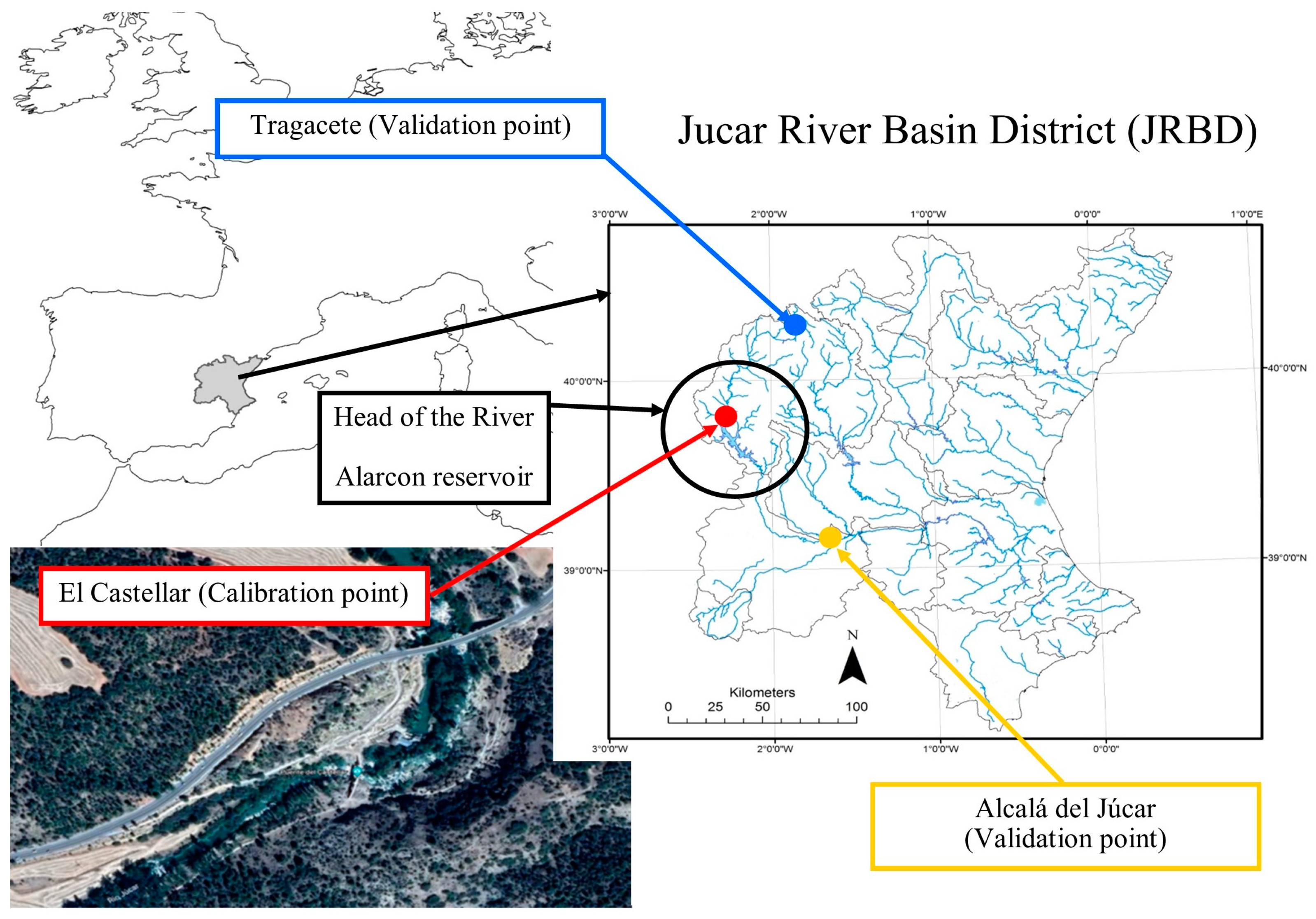
2.1. Jucar River

Jucar River is the main river of the Jucar River Basin District (JRBD) (around 43,000 km²) that is located on the Mediterranean side of the Iberian Peninsula. The JRBD provides water for water supply and irrigation to around 5.5 million inhabitants. Specifically, the river stretch studied corresponds to a cold-water fish habitat and is located upstream of the main water regulation reservoir of the JRBD (Figure 1), the Alarcón reservoir (capacity 1118 hm³), which represents a strategic reserve for drought management in the JRBD.

Common trout is a cold-water fish species present in this stretch; it is medium-sized (less than 100 cm in length) with a maximum weight of 20 kg. In this stretch, there is a water quality station from JRBD, El Castellar, with monthly data from 1998 to 2020 that include water temperature, dissolved oxygen, and others. The model was validated in two other points in this river (Tragacete and Alcalá del Júcar). Climate data are obtained from the nearest meteorological station, Cuenca, from the Spanish Meteorological Agency (AEMET, Version OpenData2.0), with mean monthly data of air temperature, wind speed, relative humidity and air pressure (

Table 1. Water temperature from JRBD (El Castellar) and climate data from Aemet (Cuenca station) (average values from monthly data for the period 1998 to 2020).

Month	Water Temperature (°C)	Air Temperature (°C)	Wind Speed (m/s)	Relative Humidity (%)	Air Pressure (Hpa)
January	6.4	9.7	1.35	73	914.9
February	7.8	11.3	1.24	67	916.3
March	10.5	16.0	2.04	60	907.8
April	12.8	17.5	1.92	60	906.8
May	15.4	18.8	1.91	56	909.5
June	18.9	23.4	2.15	48	908
July	21.7	28.1	2.04	41	910.4
August	21.5	27.0	1.81	45	909.0
September	19.3	25.2	1.70	55	910.8
October	14.7	17.8	1.62	67	909.9
November	10.3	13.2	1.42	73	912.7
December	8.0	12.9	1.64	76	906.2

).

The mean monthly air temperature is always higher than water temperature, ranging between 9.7 °C in January and 28.1 °C in July, due to groundwater contributions with cooler water to the river in summer and the snowmelt in winter. The mean monthly water temperature ranges from 6.4 °C in winter to 21.7 °C in July, which is remarkably close to the monthly thermal limit for the common trout estimated in 21.8 °C [29], so this stretch is especially vulnerable to changes in water temperature. The wind speed is between 1.24 and 2.15 m/s with a relative humidity of around 60% and an atmospheric pressure of around 901 hPa (altitude 830 masl.).

In snow-fed river basins such as mountainous watersheds, snowmelt is more relevant than changes in air temperature [68]. Rain-dominated streams, associated with low-elevation watersheds, are five to eight times more sensitive to variation in the summer air temperature compared to streams draining steeper topography whose flows were dominated by snowmelt [69]. The Jucar River catchment only has snow cover from December to March, so the Jucar River is rain-dominated in the rest of the year. For this reason, the snow component is not relevant during the summer, when warmer water temperatures and the future increase due to climate change will affect the cold-water species’ habitats.

Mean daily solar radiation, direct and diffuse (Figure 2), for the specific location is obtained from Photovoltaic Geographical Information System (PVGIS, Version 5.2) [70]. Solar irradiance, an instantaneous amount of energy from the sun (power, W/m²), is made up of direct irradiance and diffuse irradiance. The maximum value of direct irradiance occurs in July with 774 W/m², while the maximum diffuse irradiance occurs in June with 229 W/m². Irradiation (energy, kWh/m²/day) is the sum of irradiance (W/m²) during a day and is also formed by direct and diffuse irradiation that reaches water.

2.2. Methodology and Thermal Model

The daily river water temperature (RWT) model developed [71] is based on the formulation of river energy balance [72,73] adapted according to various authors, such as ref. [48]. Its purpose is to evaluate the change that occurs in RWT on a daily scale from incoming and outgoing energy balance (Figure 3).

The model is calibrated by comparing the daily temperature results in the year with the average water temperature values observed in each month. From the daily results of the model, the average monthly results are obtained, which are used to calculate the following statistical indicators: Nash–Sutcliffe Efficiency (NSE) coefficient, Kling–Gupta Efficiency (KGE) and bias.

$$NSE=1-{\displaystyle \frac{{\sum }_{t=1}^{12}{(T}_{obs,t}-T_{sim,t}{)}^2}{{\sum }_{t=1}^{12}{(T}_{obs,t}-T_{obs}{)}^2}}$$

(1)

where

T_obs,t (°C) is the observed RWT value at month (t);

T_sim,t (°C) is the simulated RWT value at month (t);

T_obs (°C) is the simulated RWT value at month (t);

T_sim (°C) is the simulated RWT value at month (t).

$$KGE=1-\sqrt{(r-1{)}^2+(\alpha -1{)}^2+(\beta -1{)}^2}$$

(2)

where

$r$ is the Pearson correlation coefficient;

$\alpha$ is a term representing the variability of prediction errors;

$$\alpha ={\displaystyle \frac{{\sigma }_s}{{\sigma }_o}}$$

(3)

${\sigma }_s$ is the variance of the simulated time series;

${\sigma }_o$ is variance of the observed time series;

β is a bias term.

$$\mathsf{\beta }= {\displaystyle \frac{Tsim-Tobs}{Tobs}}$$

(4)

$$Relative Bias= {\displaystyle \frac{Tsim-Tobs}{Tobs}}\times 100\%$$

(5)

The range of values for Nash–Sutcliffe Efficiency (NSE) validation varies from −∞ to 1. A value of 1 shows a perfect prediction, while a value of 0 suggests that the model is no better than using the observed mean. Negative values show that the model is less precise than the observed mean.

On the other hand, a KGE value of 1 indicates a perfect fit between the simulations and observations. Values closer to 1 are better, while negative values indicate a poor fit.

Finally, regarding relative bias, a positive relative bias indicates that the estimated value is greater than the true value, while a negative relative bias indicates that the estimated value is lower.

The model has been developed to reproduce the behavior in the “El Castellar” section of the river. The model is calibrated at that point only by modifying the shadow percentage. The shadow percentage obtained is in turn validated with the QBR index.

Furthermore, the validation of the model is carried out by applying the same model without modifications in the formulation in two other points of the Júcar River (cross-validation or proxy basin test), where to reproduce the water temperature in those sections of the river, you have only to adjust the shadow percentage (Tragacete and Alcalá del Júcar). The adjusted shadow percentage is compared with the degree of existing vegetation in the river in those sections and validated with the QBR values for each section.

The model proposed only has one parameter, shadow river percentage, which is associated with riparian vegetation head, river wide and river orientation.

The shadow parameter is fitted manually, trying to reduce bias, Nash and KGE coefficients. The leaf cover ranges from 10% in winter to 100% considering the leaf growth; these values are not calibrated in the model.

This parameter only affects the direct short-wave irradiation amount that reaches water, in a proportional manner, reducing this term depending on the amount of shadow, considering that all direct short-wave irradiation reaches water for 0% of shadow and zero direct irradiation reaches water for 100% of shadow. The net daily energy balance, Qn (kWh/m²/day), is obtained between energy inputs less energy outputs as follows (Equation (1)):

$$Qn =Ks+Law-Lwa\pm Qevap\pm Qcon+Win-Wout$$

(6)

where Ks (kWh/m²/day) is the net short-wave radiation that corresponds with solar irradiation less short-wave albedo, including direct and diffuse solar radiation to the water; Law (kWh/m²/day) is long-wave radiation emission from air to water; Lwa (kWh/m²/day) is long-wave water radiation emission from water to air; Qevap (kWh/m²/day) is latent heat (energy required during a change in state without a change in temperature) that corresponds with evaporation and condensation and depends on wind velocity and air vapor pressure; Qcon (kWh/m²/day) is sensible heat and is associated with conduction and convection phenomena, the heat exchange process between bodies with different temperatures that are in direct contact; Win is the energy amount that enters with the flow and Wout is the energy amount that goes out with the water; under steady-state conditions and a short stretch, the two components Win and Wout are considered to be equal and are compensated.

The net long-wave radiation air to water (Law) depends on air temperature, so when the air temperature increases, Law also rises, and the total energy inputs to water are increased. After that, to recover the energy equilibrium, it is necessary to increase the water temperature to emit more heat by the terms related to water temperature: net long-wave radiation water to air (Lwa), sensible heat (evaporation) (Qevap) and latent heat (convective) (Qcon).

Daily (i) water temperature T_w,i (Equation (2)) is obtained by adding water temperature variation (ΔT) to the previous water temperature T_w,i−1. Water temperature variation (ΔT) is obtained by iterations (Equation (3)) from energy balance Qn (kW/m²/day), river depth (m), water density ρ_w (1000 kg/m³) and water specific heat c_pw (0.001163 kWh/kg °C).

One of the keys to water temperature is flow, which is a function of the depth.

$$T_{W,i}=T_{W,i-1}+∆T$$

(7)

$$∆\mathrm{T}={\displaystyle \frac{dT}{dt}}={\displaystyle \frac{Q_n}{{\rho }_w·d·c_{pw}}}$$

(8)

In addition, based on studies [30], fundamental variables are the air temperature and the combination of air temperature and water temperature to predict the water temperature.

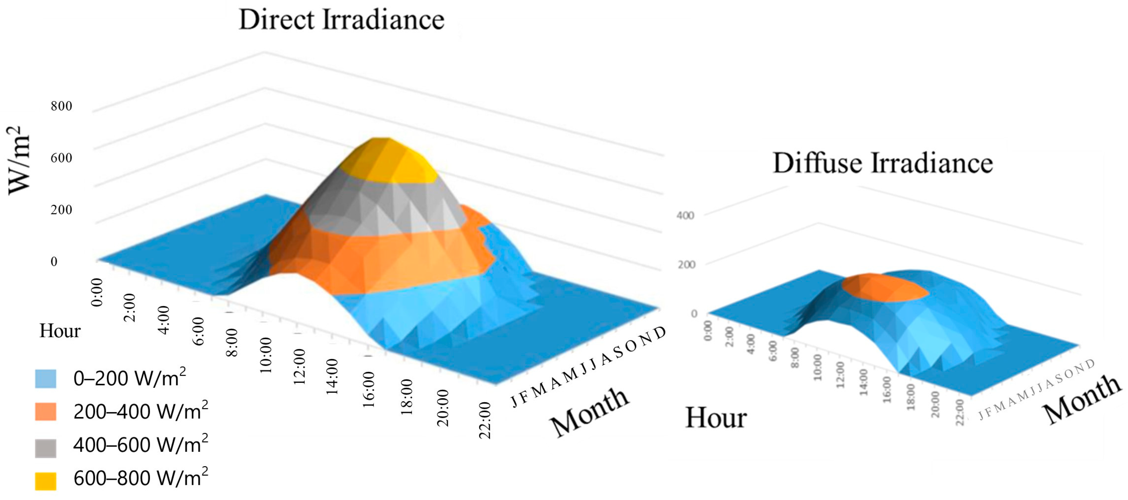
2.2.1. Net Short-Wave Radiation (Ks)

Net short-wave radiation (Equation (4)), Ks (kWh/m²/day), is the downward solar irradiation at the ground level, including direct and diffuse irradiation (Kdirect, Kdiffuse in kWh/m²/day) obtained from PVGIS, less short-wave radiation reflected back to the atmosphere (named albedo A_S).

$$Ks = \left(\right[Kdirect·\left(1-Shadow\right)]+Kdiffuse) ·(1-A_S)$$

(9)

Shadow is the percentage of shadow over the river and varies from zero (no shadow) to one (100% shadow). Albedo depends on the water surface reflectivity, which is related to surface color (darker surface produces smaller albedo), chlorophyll concentration, water depth, and solar angle (water has a higher albedo for a low solar angle). It typically ranges for surface waters between 0.01 and 0.10, and it is considered 0.05 for this river.

2.2.2. Air to Water Net Long-Wave Radiation (Law)

Net long-wave radiation from air to water, Law (kWh/m²/day), is the heat emission from air, corresponding with radiation emitted by any material with a temperature above absolute zero by Stefan–Boltzmann’s law of blackbody radiation (Equation (5)) less long-wave radiation reflected (long-wave albedo A_L).

$$Law= Ea·\sigma ·{\left(Ta+273.15\right)}^4·kday·(1-A_L)$$

(10)

where Ea is the atmospheric emissivity (W/m²) that depends on air temperature and air vapor pressure; σ is the Stefan–Boltzmann constant 5.670373 × 10⁻⁸ (W/m²/K⁴); Ta is the daily mean air temperature (°C); A_L is the long-wave albedo, and it is considered as 0.03 [73]; and kday is the conversion coefficient to integrate irradiance across the entire day (60 × 60 × 24/1000/60/60).

Atmospheric emissivity Ea is determined for each day using different formulations (

Table 2. Formulations for atmospheric emissivity.

$Ea=0.55+0.065 ·\sqrt{e_a}$	[74]
$Ea=9.365 ·{10}^{-6}·{\left(T_a+273.15\right)}^2$	[75]
$Ea=1-0.26·Exp\left(-7.77·{10}^{-4}·\left(273.15-T_a\right)\right)$	[76]
$Ea=1.24·{\left({\displaystyle \frac{e_a}{T_a+273.15}}\right)}^{0.14}$	[77]
$Ea=0.7+5.95·{10}^{-5}·e_a·exp\left({\displaystyle \frac{1500}{T_a+273.15}}\right)$	[78]
$Ea=0.684+0.056·e_a$	[79]

), which depend on the air temperature (Ta, °C) and air vapor pressure (e_a, mb = hPa). The maximum range for the estimated Ea by different authors is around 10% of the average, so a mean value is applied. The mean value obtained during the year varies from 0.78 to 0.84 with a global mean annual value of 0.81.

Here, air vapor pressure e_a (Equations (6) and (7)) (mb = hPa) is obtained from the air temperature Ta (°C), relativity air humidity RH (%), and empirical coefficients r₁ = 6.12 (mb), r₂ = 17.27 and r₃ = 237.3 (°C), as

$$e_s\left(T_a\right)=r_1·exp\left({\displaystyle \frac{r_2·T_a}{T_a+r_3}}\right)$$

(11)

$$e_a\left(T_a\right)=e_s\left(T_a\right)·{\displaystyle \frac{RH}{100}}$$

(12)

2.2.3. Water to Air Long-Wave Radiation (Lwa)

Long-wave water radiation, Lwa (kWh/m²/day), from water to air (Equation (8)) can also be calculated using the Stefan–Boltzmann law as follows:

$$Lwa=Ew·\sigma ·{\left(Tw+273.15\right)}^4·kday$$

(13)

where Tw is the water temperature (°C) and Ew is the water emissivity that depends on the water transparency or surface smoothness and ranges between 0.9 and 0.99 [73]. Ew is 0.96 for pristine water, so 0.97 will be used in this river.

2.2.4. Latent Heat (Qevap)

Latent heat, Qevap (kW/m²/day), is related to evaporation and condensation and depends on the wind velocity and air vapor pressure (Equation (9)).

This phenomenon is produced by energy added or removed from a substance, which causes a change in state without any change in temperature. Evaporation is proportional to the difference between air vapor saturation es (mb) (Equation (6)) and air vapor pressure ea (mb) (Equation (7)):

$$Qevap=f\left(u\right)·(es-ea) · kday$$

(14)

where f (u) is the wind speed function (W/m²/mb), which is selected as a daily mean value from the different f (u) formulations. The annual mean value is 9.06 (W/m²/mb) and ranges during the year from 7.70 to 10.07 (W/m²/mb).

2.2.5. Sensible Heat (Qcon)

Sensible heat, Qcon (kW/m²/day), is associated with conduction and convection phenomena, and this is the heating exchange process between different temperature bodies in direct contact, water and air. It depends on the temperature difference between air and water, the wind velocity, the relative air pressure and Bowen’s coefficient (Equation (10)).

$$Qcon=Cb·(Pa/Po)·f\left(u\right)·(Ta-Tw)·kday$$

(15)

where Cb is Bowen’s coefficient ≈ 0.62 (mb/°C); Pa is air pressure (mb); Po is the reference air pressure 1013 (mb); f (u) is the wind speed function (W/m²/mb); Ta is the air temperature (°C); and Tw is the water temperature (°C).

3. Results and Discussion

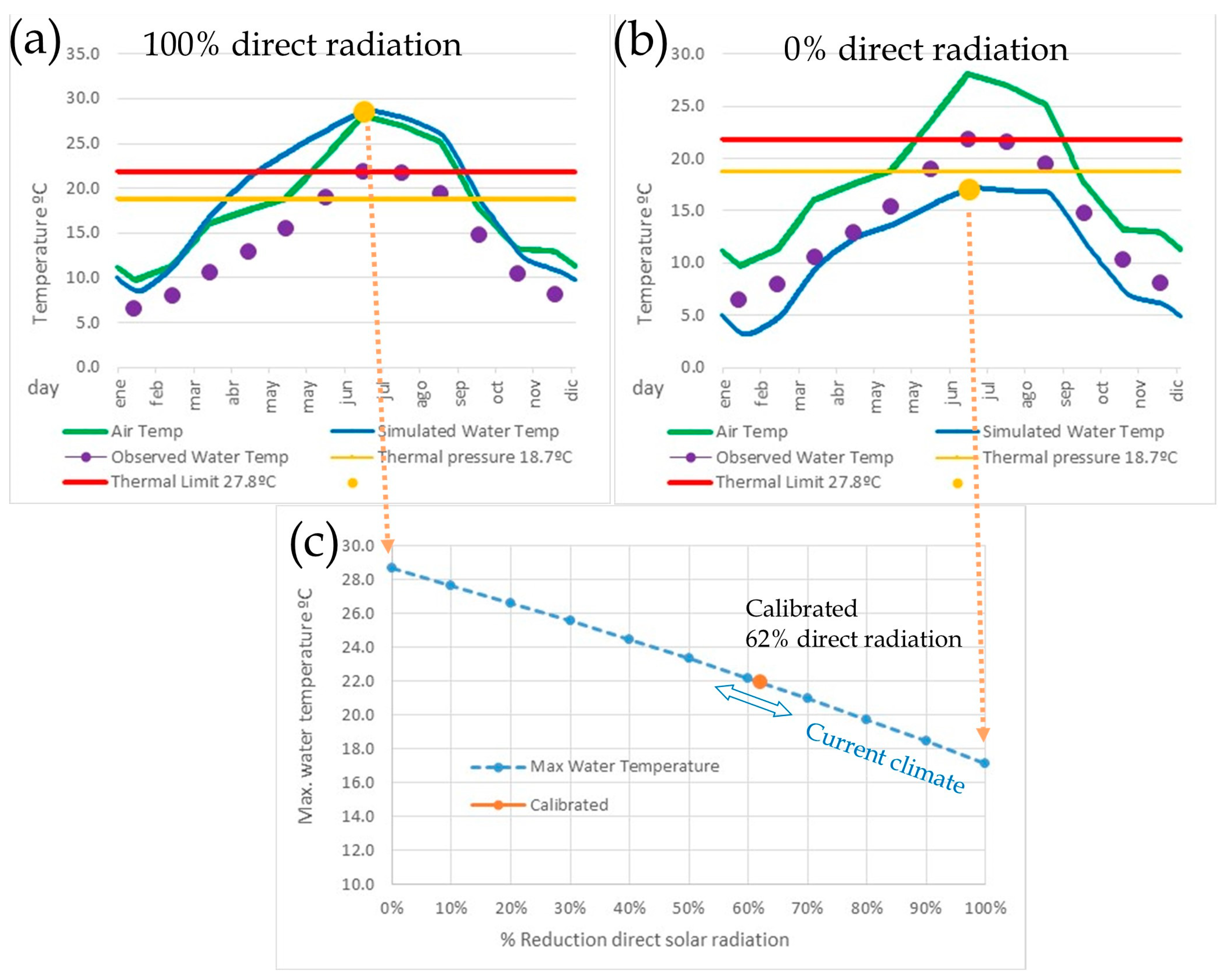
3.1. Model Calibration and Water Energy Balance

A daily model has been calibrated in the Jucar River, upstream of Alarcón reservoir in “El Castellar”, where the state of riparian vegetation is intermediate with 65 points for the QBR index [80]. The QBR index (Riparian Forest Quality) classification ranges from <25 for extreme degradation, bad quality, to >95 for riparian habitat in natural condition. The model results are independent of river depth in the habitual range of these types of rivers, between 0.5 and 5 m.

The results show that for a 62% vegetation cover percentage (Figure 4), there is a good fit between simulated and monthly mean observed data with a 0.93 Nash–Sutcliffe efficiency coefficient (NSE) [81] that indicates a very good model fit [82], a 0.90 Kling–Gupta efficiency index KGE [83] and a relative bias of 0.04.

The calibrated value of 62% of shadow by vegetation adjusts very well to a QBR index of 65 points out of a rating of 95 points for a habitat with well-developed natural vegetation cover (95WD). In this way, the parameter is validated.

Taking seasonal influence into account, the water temperature in winter is slightly higher (+1 °C), and in summer, it stays the same. Furthermore, the Nash indicator continues to be good, dropping from 0.93 to 0.87. This is not significant for the study objective but could be an important extension of the analysis.

The water temperature model is calibrated with real observed water temperature data, so this water temperature is the result of the current land uses of the entire catchment. The model’s purpose is to evaluate the effect of riparian vegetation on the river water temperature. In the case of evaluating the effect of changes in the land uses of the basin, other models, like SWAT [84], can provide information about how changes in land uses can affect the water temperature.

This vegetation cover percentage obtained during calibration, 62%, corresponds with a realistic value for this area due to the intermediate state of the riparian vegetation, QBR = 65. The model was validated in two other points in this river. The first one is located 100 km upstream in Tragacete with cooler conditions, where for a well-developed riparian vegetation QBR = 85, the best model results are obtained for 98% of coverage with relative bias = −0.02, Nash = 0.38 and KGE = 0.30. The second one is located 130 km downstream in Alcala del Jucar with hotter conditions, where the riparian vegetation is bad, QBR = 52, and the best results are obtained for 50% of coverage with relative bias = −0.03, Nash = 0.50 and KGE = 0.38.

For the upstream section, the calibrated value of 98% shade by vegetation adjusts very well to a QBR index of 85 points (95WD). For the other section, the calibrated value of 50% shade by vegetation adjusts very well to a QBR index of 52 points (95WD). In both cases, it is validated.

The water temperature exceeds the thermal pressure level for brown trout (>18.7 °C) in summer months for 120 days from June to September, being remarkably close to the monthly thermal tolerance limit, 21.8 °C [29], for 15 days in July.

Snow cover and ice phenomena are relevant factors in water temperature, especially in snow-fed river basins. The Jucar River catchment only has snow cover from December to March, so this component is not relevant during summer when warmer water temperatures and the future increase due to climate change will affect the cold-water species’ habitats. This analysis is focused on the worst condition for cold-water habitats that is produced in the warmer months of summer when the river water temperature is higher.

Energy inputs to water are short-wave radiation and sensible heat (related to air–water contact) because the air temperature is greater than the water temperature, so there is a positive balance of convective heat from air to water. Short-wave radiation, which is direct radiation and diffuse radiation sum, is the main input and varies from 1.32 kWh/m²/day in December to 4.25 kWh/m²/day in June (Figure 5) with a mean annual value of 2.82 kW/m²/day (

Table 3. Water energy balance in El Castellar with 62% of shadow (kWh/m²/day).

Shadow 62%	COMPONENT			GLOBAL
	Short-wave Radiation	2.82
	Rs albedo	−0.14
	Ks		2.68
	Qcon Convective heat (air-water)		0.47
TOTAL INPUT				3.15
	Lwa Long-wave Water to Air Emission	−9.04
	Law Long-wave Air to Water Emission	7.82
	Law albedo	−0.23
	LW Balance (Ls + Lb)		−1.45
	Qevap evaporation heat		−1.69
TOTAL OUTPUT				−3.14

). Sensible heat varies from 0.19 kWh/m²/day in May to 0.75 kWh/m²/day in July with an average value of 0.47 kWh/m²/day.

Both main energy outputs, latent heat (Qevap) and long-wave balance (related to long-wave emissions of air and water), have similar annual values. Latent heat, associated with evaporation, has an annual mean value of 1.69 kWh/m²/day, which varies between 0.48 kWh/m²/day in January and 3.47 kWh/m²/day in July, which are months when evaporation is higher. Long-wave balance is produced from water to air with an annual mean of 1.45 kWh/m²/day, because although the air temperature is higher than the water temperature, the air emission coefficient (around 0.79) is significantly lower than the water emission coefficient (0.97).

3.2. Vegetation Coverage and Water Temperature

The direct radiation amount reaching the water has an incredibly significant influence on river water temperature (RWT) (Figure 6c). In the case of 100% direct solar radiation, and a 0% reduction in direct solar irradiation (Figure 6a), the maximum RWT in July is 28.6 °C, and in the case of 0% of direct solar radiation (Figure 6b), the maximum RWT is 17.1 °C for the same month. The theoretical maximum RWT amplitude is 11.5 °C depending on the amount of direct solar radiation that reaches the river (Figure 6c).

River flow affects water temperature in the way that a larger flow has more thermal inertia and requires more time to change its temperature. The river flow depends on the water velocity and the wetted area, which also depends on the river width and depth. River depth is included in the model formulation in Equation (3). The Jucar River flow oscillation produces a depth range between 0.5 and 2.5 m, so in these conditions for a large distance, stationary state, the river water temperature is highly independent of the flow. The flow, the amount of water that enters the stretch, has an influence on the distance needed to reach the stationary state for water temperature.

On the other hand, the model results show that to obtain a lower temperature, a higher depth of 10 m would be necessary, which is something that is not possible for the geomorphological conditions of the Jucar River and the other characteristics.

The river flow has been considered, but as shown in the following figure, it is not significant for the depths of the Júcar River (0.5–2.5 m).

The results show the significant importance in the amount of direct solar radiation that reaches the water and how modifying this input can change significantly the RWT and therefore the effects in the river ecosystem. On average, each reduction of 10% in direct solar irradiation reduces the river water temperature by 1.2 °C.

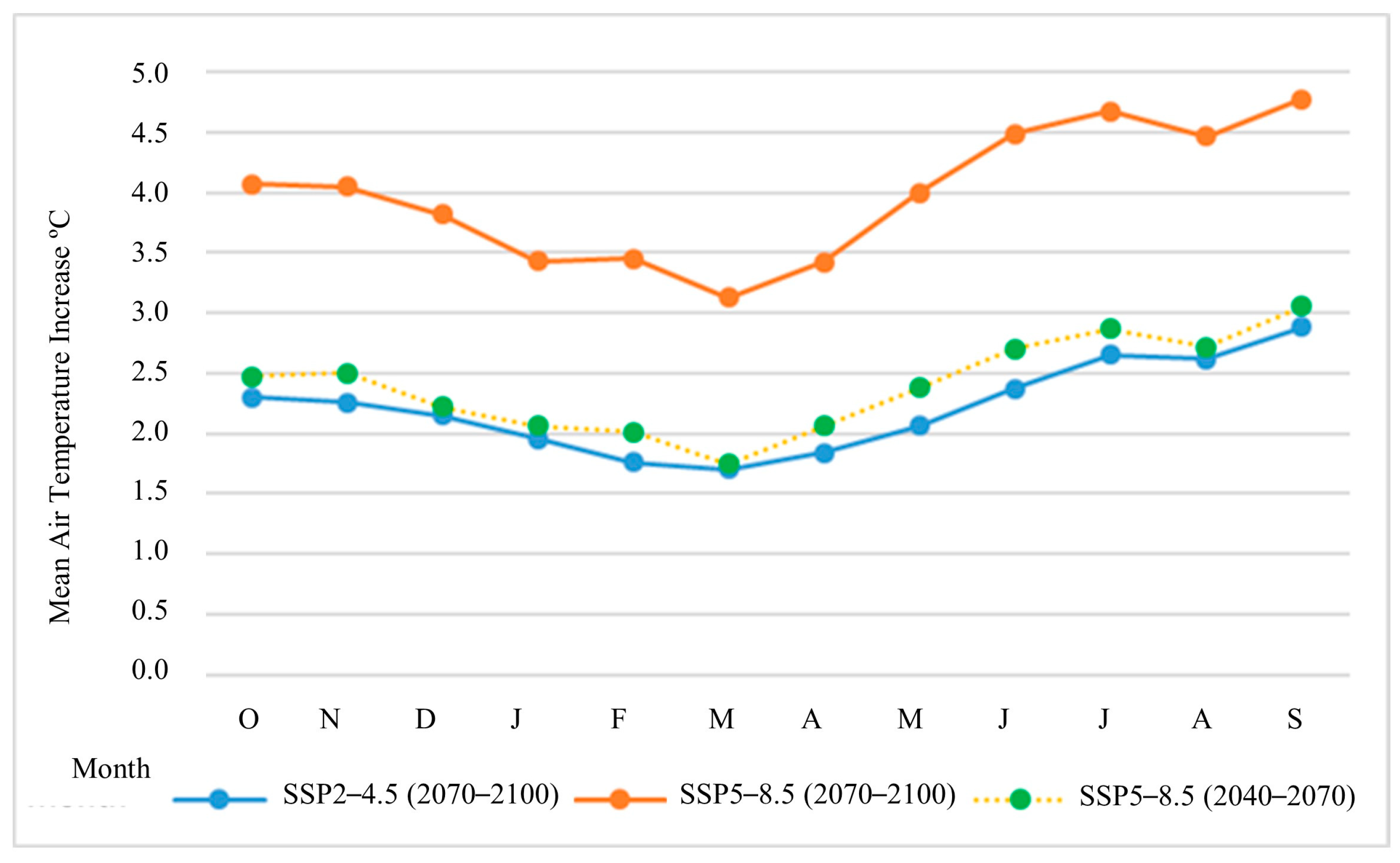
3.3. Water Temperature Under Climate Change Scenarios

The air annual mean temperature will rise between 2 °C in the intermediate scenario SSP2-4.5 [84,85] and 4 °C in the high scenario SSP5-8.5 in the long term (2070–2100) in the JRBD (Figure 7). Only scenarios with radiative forcing below 1.9 W/m² will produce an increase in air temperature lower than 1.5 °C, which is established as the goal in the 2015 Paris Agreement [86]. The air temperature increase will be higher in summer with 2.7 °C (SSP2-4.5) and 4.7 °C (SSP5-8.5).

Both scenarios increase air temperature during the 21st century with a higher rate for the SSP5-8.5 scenario, so the intermediate period (mid-term 2040–2070) of the SSP5-8.5 scenario has a similar increase in air temperature to the SSP2-4.5 scenario for the long-term period; in this way, conclusions obtained for the long-term SSP2-4.5 scenario can also be valid to the mid-term of the SSP5-8.5 scenario.

Under the long-term SSP2-4.5 scenario, the air temperature increases 2.6 °C in July (Figure 8) and produces a water temperature increase of 1.6 °C in the same month. The water temperature exceeds the stress threshold for 150 days and the thermal limit for 95 days (3 months, June, July and August), so in these conditions, the river loses its habitat for the common trout. Comparable results can be established for the mid-term SSP5-8.5 scenario (2040–2070).

In the long-term SSP5-8.5 scenario (Figure 9b), the air temperature increase of 4.6 °C in July produces a water temperature increase of 2.8 °C; in addition the stress threshold is exceeded for 175 days, and the thermal limit is exceeded for 120 days (4 months). As in the previous scenario, the habitat for the common trout has been lost.

The results obtained for the Jucar River upstream of the Alarcon reservoir, El Castellar, sustain that the water temperature overcomes the thermal limit for the brown trout habitat for four months and exceeds the affecting limit for six months a year, which makes the habitat unviable for this species (

Table 4. Water energy balance (and change) in El Castellar with 62% of shadow under SSP5-85 scenario (kWh/m²/day).

Scheme 62.	COMPONENT			GLOBAL
	Short-wave radiation	2.82
	Rs albedo	−0.14
	Ks		2.68 (+0.00)
	Qcon convective heat (air–water)		0.58 (+0.11)
TOTAL INPUT				3.26 (+0.11)
	Lwa Long-wave water to air emission	−9.43
	Law long-wave air to water emission	8.46
	Law albedo	−0.25
	LW balance (Ls + Lb)		−1.23 (+0.22)
	Qevap evaporation heat		−2.04 (−0.35)
TOTAL OUTPUT				−3.26 (−0.11)

). These results confirm that this stream will be inhabitable for common trout, as it is indicated in previous works [71], as it is obtained in other rivers, where fish habitats and river ecosystems are threatened by climate warming with some endangered species such as brown trout being particularly vulnerable [87].

Under climate change scenarios, greater air temperature increases sensible (conduction and convective) heat flux from air to water (+0.11 kWh/m²/day) and long-wave radiation from air to water. In addition, long-wave heat fluxes are strongly changed, decreasing the net flux from water to air that is partially compensated with more evaporation.

3.4. Nature-Based Measures to Reduce Water Temperature

Reducing direct solar irradiation can compensate for air temperature by climate change (CC), which can be obtained by nature-based measures like increasing shadow formed by a more dense and high riparian vegetation. The relationship curve between the direct solar radiation reduction and river water temperature in July is displaced to the right under CC conditions with a hotter air temperature in July (Figure 9). To maintain the maximum river water temperature in July under the thermal limit, the direct solar radiation must be reduced from 62% in the current conditions to 76% for the scenario SSP2-4.5 and to 87% for the scenario SSP5-8.5 at the end of the century.

Figure 9. Air and water temperature under climate change scenarios for the long-term (2070–2100), (a) SSP2-4.5 and (b) SSP5-8.5.

Figure 9. Air and water temperature under climate change scenarios for the long-term (2070–2100), (a) SSP2-4.5 and (b) SSP5-8.5.

For the SSP2-4.5 scenario, reducing direct solar radiation from 62% to 76% implies that direct solar radiation that reaches the water is reduced from 2.82 to 2.36 kWh/m²/day, which represents a reduction of 0.46 kWh/m²/day (Figure 10). In the case of the SSP5-8.5 scenario, direct solar radiation changes to 2.00 kWh/m²/day, which represents a reduction of 0.82 kWh/m²/day. The reduction in heat input from direct solar radiation is one of the main measures to compensate air temperature rise, as it is indicated by other authors [88]. It is evident that vegetation cover favors the adaptation of rivers to CC, and the use of models, like the model presented, can help to define how much vegetation (or shadow percentage) is necessary to maintain the habitat under different CC scenarios.

Riparian shading has a significant role in reducing the temperature in rivers in the same magnitude as the RWT increases by CC. In Austrian rivers, for maximum water temperatures, a downstream warming of 3.9 °C was observed in the unshaded areas, which was followed by a downstream cooling of 3.5 °C in shaded areas, and the water temperature directly responded to the air temperature and cloudiness [88]. The results obtained in basins in the United Kingdom and Denmark [89] indicate the need to use riparian strips, which are not necessarily extensive, to reduce the water temperature where salmonids prevail. Specifically, in the experiment carried out during July, August and September, a period of maximum air temperature and vegetation cover, 100 m of riparian forest reduced the water temperature of streams by up to 1° C compared to the temperature of a riverbed opened. If the length of the riparian forest extends up to 500 m and the vegetation cover is between 75 and 90%, the shading effect is increased, and the temperature can be reduced by 2–3 °C. For these reasons, the work indicates that increasing the vegetation cover in relatively short areas can be useful [89].

Mediterranean rivers, also, are characterized by torrential rains that produce heavy, dangerous and fast floods, so current river restoration strategies consist of widening channels and having shrubby vegetation on riverbanks to facilitate channels drainage, increasing river capacity, and reducing floods.

This type of restoration produces little shading in water, so direct solar radiation is increased, and any further river water temperature rise will reduce the habitat for cold-water species. In this context, it is necessary to find nature-based solutions where rivers have the capacity to avoid floods, and riparian vegetation provides enough shadow to the water to maintain a cold-water fish habitat, especially under CC conditions.

4. Conclusions

Climate change will increase the air and water temperature in lakes and rivers, considerably affecting river ecosystems. Cold-water fish species, such as trout and salmon, are extremely sensitive to warm water, which can promote specific diseases or prevent reproduction.

Different studies provide evidence that wooded riparian zones can reduce stream temperatures, particularly in terms of maximum temperatures, but without quantifying the density of vegetation necessary to address climate change. The main objective was to create a simulated model that relates the temperature of the river with the shadow generated by the riverside vegetation.

The model was calibrated and applied in a river stretch located in the upper Jucar River, in the Mediterranean area, and validated in other two stretches of the same river located 100 km upstream and downstream for cooler and hotter conditions. The model performance values for this point for 62% of cover are relative bias = 0.02, Nash = 0.96 and KGE = 0.96, so the model can be considered a good model for this purpose.

The results indicate that the degree of shadow coverage on rivers is a crucial factor in the final temperature of water, so that the river water temperature in current conditions can vary from 17.1 to 28.6 °C depending on the percentage (0% to 100%) of direct solar radiation that reaches the water. On average, each reduction of 10% in direct solar irradiation reduces the river water temperature by 1.2 °C.

Under climate change scenarios, air temperature increases will be higher in summer with 2.7 °C (SSP2-4.5) and 4.7 °C (SSP5-8.5); the way to reduce that temperature by increasing the percentage of shadow will be the key in the future.

Nature-based solutions that consist of improving shadow with a well-developed riparian vegetation can reduce the direct solar radiation to the water and can compensate for the air temperature increase by climate change. This nature-based solution also contributes to improving the river ecosystem in many ways. For the case analyzed, it is possible to maintain river water temperatures in the current values, increasing the shadow from 62% to 76% for the SSP2-4.5 scenario and to 87% for the SSP5-8.5 scenario.

References

1. Kelleher, C.A.; E Golden, H.; Archfield, S.A. Monthly river temperature trends across the US confound annual changes. Environ. Res. Lett. 2021, 16, 104006–104010. [Google Scholar] [CrossRef] [PubMed]
2. Jastram, J.D.; Rice, K.C. Air- and Stream-Water-Temperature Trends in the Chesapeake Bay Region, 1960–2014. U.S. Geological Survey Open-File Report 2015-1207. 2015. Available online: https://pubs.er.usgs.gov/publication/ofr20151207 (accessed on 30 October 2024).
3. Liu, S.; Xie, Z.; Liu, B.; Wang, Y.; Gao, J.; Zeng, Y.; Xie, J.; Xie, Z.; Jia, B.; Qin, P.; et al. Global river water warming due to climate change and anthropogenic heat emission. Glob. Planet. Chang. 2020, 193, 103289, ISSN 0921-8181. [Google Scholar] [CrossRef]
4. Zhu, S.; Luo, Y.; Graf, R.; Wrzesinski, D.; Sojka, M.; Sun, B.; Kong, L.; Ji, Q.; Luo, W. Reconstruction of long-term water temperature indicates significant warming in Polish rivers during 1966–2020. J. Hydrol. Reg. Stud. 2022, 44, 101281, ISSN 2214-5818. [Google Scholar] [CrossRef]
5. Isaak, D.J.; Wollrab, S.; Horan, D.; Chandler, G. Climate change effects on stream and river temperatures across the northwest U.S. from 1980–2009 and implications for salmonid fishes. Clim. Chang. 2011, 113, 499–524. [Google Scholar] [CrossRef]
6. Basarin, B.; Lukić, T.; Pavić, D.; Wilby, R.L. Trends and Multi-Annual Variability of Water Temperatures in the River Danube, Serbia. Hydrol. Process. 2016, 30, 3315–3329. [Google Scholar] [CrossRef]
7. Arora, R.; Tockner, K.; Venohr, M. Changing river temperatures in northern Germany: Trends and drivers of change. Hydrol. Process. 2016, 30, 3084–3096. [Google Scholar] [CrossRef]
8. O’Reilly, C.M.; Sharma, S.; Gray, D.K.; Hampton, S.E.; Read, J.S.; Rowley, R.J.; Schneider, P.; Lenters, J.D.; McIntyre, P.B.; Kraemer, B.M.; et al. Rapid and highly variable warming of lake surface waters around the globe. Geophys. Res. Lett. 2015, 42, 10773–10781. [Google Scholar] [CrossRef]
9. Sharma, S.; Gray, D.K.; Read, J.S.; O’Reilly, C.M.; Schneider, P.; Qudrat, A.; Gries, C.; Stefanoff, S.; Hampton, S.E.; Hook, S.; et al. A global database of lake surface temperatures collected by in situ and satellite methods from 1985–2009. Sci. Data 2015, 2, 150008. [Google Scholar] [CrossRef]
10. NOAA. Great Lakes water level observations. National Oceanic and Atmospheric Administration; NOAA: Washington, DC, USA, 2021. [Google Scholar]
11. Graf, R.A. Multifaceted analysis of the relationship between daily temperature of river water and air. Acta Geophys. 2019, 67, 1–16. [Google Scholar] [CrossRef]
12. Graf, R.; Wrzesiński, D. Relationship Between Water Temperature of Polish Rivers and Large-Scale Atmospheric Circulation. Water 2019, 11, 1690. [Google Scholar] [CrossRef]
13. Benyahya, L.; Caissie, D.; St-Hilaire, A.; Ouarda, T.B.; Bobée, B. A Review of Statistical Water Temperature Models. Can. Water Resour. J. Rev. Can. Ressour. Hydriques 2007, 32, 179–192. [Google Scholar] [CrossRef]
14. Watts, G.; Battarbee, R.W.; Bloomfield, J.P.; Crossman, J.; Daccache, A.; Durance, I.; Elliott, J.A.; Garner, G.; Hannaford, J.; Hannah, D.M.; et al. Climate change and water in the UK—past changes and future prospects. Prog. Phys. Geogr. 2015, 39, 6–28. [Google Scholar] [CrossRef]
15. Wagner, T.; Midway, S.R.; Whittier, J.B.; DeWeber, J.T.; Paukert, C.P. Annual Changes in Seasonal River Water Temperatures in the Eastern and Western United States. Water 2017, 9, 90. [Google Scholar] [CrossRef]
16. Rajesh, M.; Rehana, S. Impact of climate change on river water temperature and dissolved oxygen: Indian riverine thermal regimes. Sci. Rep. 2022, 12, 9222. [Google Scholar] [CrossRef] [PubMed]
17. van Vliet, M.T.; Franssen, W.H.; Yearsley, J.R.; Ludwig, F.; Haddeland, I.; Lettenmaier, D.P.; Kabat, P. Global river discharge and water temperature under climate change. Glob. Environ. Chang. 2013, 23, 450–464, ISSN 0959-3780. [Google Scholar] [CrossRef]
18. Hardenbicker, P.; Viergutz, C.; Becker, A.; Kirchesch, V.; Nilson, E.; Fischer, H. Water temperature increases in the river Rhine in response to climate change. Reg. Environ. Chang. 2017, 17, 299–308. [Google Scholar] [CrossRef]
19. Estrela-Segrelles, C.; Mocholi-Paredes, C.; Pérez-Martín, M.A. Impact of Climate Change on Cold-Water Fish Species: Application in the Jucar River Basin District. In Proceedings of the 39th IAHR World Congress—From Snow to Sea, Granada, Spain, 19–24 June 2022. [Google Scholar] [CrossRef]
20. Michel, A.; Schaefli, B.; Wever, N.; Zekollari, H.; Lehning, M.; Huwald, H. Future water temperature of rivers in Switzerland under climate change investigated with physics-based models. Hydrol. Earth Syst. Sci. 2022, 26, 1063–1087. [Google Scholar] [CrossRef]
21. Caissie, D The thermal regime of rivers: A review. Freshw. Biol. 2006, 51, 1389–1406. [CrossRef]
22. Carraro, L.; Mari, L.; Hartikainen, H.; Strepparava, N.; Wahli, T.; Jokela, J.; Gatto, M.; Rinaldo, A.; Bertuzzo, E. An epidemiological model for proliferative kidney disease in salmonid populations. Parasit. Vect. 2016, 9, 487. [Google Scholar] [CrossRef]
23. Rahel Frank, J.; Keleher Christopher, J.; Anderson Jeffry, L. Potential habitat loss and population fragmentation for cold water fish in the North Platte River drainage of the Rocky Mountains: Response to climate warming. Limnol. Oceanogr. 1996, 41, 1116–1123. [Google Scholar] [CrossRef]
24. Eaton John, G.; Scheller Robert, M. Effects of climate warming on fish thermal habitat in streams of the United States. Limnol. Oceanogr. 1996, 41, 1109–1115. [Google Scholar] [CrossRef]
25. Estrela-Segrelles, C.; Pérez-Martín, M.A. Hazard, Exposure, Vulnerability and Risk Maps Associated with the Impact of Climate Change: Application in Júcar River Basin District. In Proceedings of the 39th IAHR World Congress—From Snow to Sea, Granada, Spain, 19–24 June 2022. [Google Scholar] [CrossRef]
26. Paillex, A.; Schuwirth, N.; Lorenz, A.W.; Januschke, K.; Peter, A.; Reichert, P. Integrating and extending ecological river assessment: Concept and test with two restoration projects. Ecol. Indic. 2017, 72, 131–141. [Google Scholar] [CrossRef]
27. Niedrist, G.H.; Füreder, L. Real-time warming of Alpine streams: (Re)defining invertebrates’ temperature preferences. River Res. Appl. 2021, 7, 283–293. [Google Scholar] [CrossRef]
28. Eaton, J.G.; McCormick, J.H.; Goodno, B.E.; O’Brien, D.G.; Stefany, H.G.; Hondzo, M.; Scheller, R.M. A Field Information-based System for Estimating Fish Temperature Tolerances. Fisheries 1995, 20, 10–18. [Google Scholar] [CrossRef]
29. Wehrly, K.E.; Wang, L.; Mitro, M. Field-Based Estimates of Thermal Tolerance Limits for Trout: Incorporating Exposure Time and Temperature Fluctuation. Trans. Am. Fish. Soc. 2007, 136, 365–374. [Google Scholar] [CrossRef]
30. Heddam, S.; Kim, S.; Mehr, A.D.; Zounemat-Kermani, M.; Ptak, M.; Elbeltagi, A.; Malik, A.; Tikhamarine, Y. Bat algorithm optimised extreme learning machine (Bat-ELM): A novel approach for daily river water temperature modelling. Geogr. J. 2023, 189, 78–89. [Google Scholar] [CrossRef]
31. Heddam, S.; Merabet, K.; Difi, S.; Kim, S.; Ptak, M.; Sojka, M.; Zounemat-Kermani, M.; Kisi, O. River water temperature prediction using hybrid machine learning coupled signal decomposition: EWT versus MODWT. Ecol. Inform. 2023, 78, 102376. [Google Scholar] [CrossRef]
32. Piccolroaz, S.; Zhu, S.; Ladwig, R.; Carrea, L.; Oliver, S.; Piotrowski, A.P.; Ptak, M.; Shinohara, R.; Sojka, M.; Woolway, R.I.; et al. Lake Water Temperature Modeling in an Era of Climate Change: Data Sources, Models, and Future Prospects. Rev. Geophys. 2024, 62, e2023RG000816. [Google Scholar] [CrossRef]
33. Sun, J.; Di Nunno, F.; Sojka, M.; Ptak, M.; Zhou, Q.; Luo, Y.; Granata, F. Long-Term Daily Water Temperatures Unveil Escalating Water Warming and Intensifying Heatwaves in the Odra River Basin, Central Europe. Geosci. Front. 2024, 15, 101916. [Google Scholar] [CrossRef]
34. Ahmadi-Nedushan, B.; St-Hilaire, A.; Ouarda, T.B.; Bilodeau, L.; Robichaud, E.; Thiémonge, N.; Bobée, B. Predicting River Water Temperatures Using Stochastic Models: Case Study of the Moisie River (Québec, Canada). Hydrol. Process. 2007, 21, 21–34. [Google Scholar] [CrossRef]
35. Zhu, S.; Piotrowski, A.P. River/Stream Water Temperature Forecasting Using Artificial Intelligence Models: A Systematic Review. Acta Geophys. 2020, 68, 1433–1442. [Google Scholar] [CrossRef]
36. Zhu, S.; Nyarko, E.K.; Hadzima-Nyarko, M. Modelling Daily Water Temperature from Air Temperature for the Missouri River. PeerJ 2018, 6, e4894. [Google Scholar] [CrossRef] [PubMed]
37. Rabi, A.; Hadzima-Nyarko, M.; Šperac, M. Modelling River Temperature from Air Temperature: Case of the River Drava (Croatia). Hydrol. Sci. J. 2015, 60, 1490–1507. [Google Scholar] [CrossRef]
38. Morrill, J.C.; Bales, R.C.; Conklin, M.H. Estimating Stream Temperature from Air Temperature: Implications for Future Water Quality. J. Environ. Eng. 2005, 131, 139–146. [Google Scholar] [CrossRef]
39. Moore, R.D. Stream Temperature Patterns in British Columbia, Canada, Based on Routine Spot Measurements. Can. Water Resour. J. 2006, 31, 41–56. [Google Scholar] [CrossRef]
40. Smith, K. The Prediction of River Water Temperatures/Prédiction des Températures des Eaux de Rivière. Hydrol. Sci. J. 1981, 26, 19–32. [Google Scholar] [CrossRef]
41. Wanders, N.; van Vliet, M.T.H.; Wada, Y.; Bierkens, M.F.P.; van Beek, L.P.H. High-Resolution Global Water Temperature Modeling. Water Resour. Res. 2019, 55, 2760–2778. [Google Scholar] [CrossRef]
42. DeWeber, J.T.; Wagner, T. A Regional Neural Network Ensemble for Predicting Mean Daily River Water Temperature. J. Hydrol. 2014, 517, 187–200. [Google Scholar] [CrossRef]
43. Punzet, M.; Voß, F.; Voß, A.; Kynast, E.; Bärlund, I. A Global Approach to Assess the Potential Impact of Climate Change on Stream Water Temperatures and Related In-Stream First-Order Decay Rates. J. Hydrometeorol. 2012, 13, 1052–1065. [Google Scholar] [CrossRef]
44. van Vliet, M.T.H.; Ludwig, F.; Zwolsman, J.J.G.; Weedon, G.P.; Kabat, P. Global river temperatures and sensitivity to atmospheric warming and changes in river flow. Water Resour. Res. 2011, 47, W02544. [Google Scholar] [CrossRef]
45. St-Hilaire, A.; Morin, G.; El-Jabi, N.; Caissie, D. Water temperature modelling in a small forested stream: Implication of forest canopy and soil temperature. Can. J. Civ. Eng. 2000, 27, 1095–1108. [Google Scholar] [CrossRef]
46. Edinger, J.E.; Duttweiler, D.W.; Geyer, J.C. The Response of Water Temperatures to Meteorological Conditions. Water Resour. Res. 1968, 4, 1137–1143. [Google Scholar] [CrossRef]
47. Caissie, D.; Satish, M.G.; El-Jabi, N. Predicting Water Temperatures Using a Deterministic Model: Application on Miramichi River Catchments (New Brunswick, Canada). J. Hydrol. 2007, 336, 303–315. [Google Scholar] [CrossRef]
48. Kalinowska, M.B. Effect of water–air heat transfer on the spread of thermal pollution in rivers. Acta Geophys. 2019, 67, 597–619. [Google Scholar] [CrossRef]
49. Dugdale, S.J.; Malcolm, I.A.; Kantola, K.; Hannah, D.M. Stream Temperature Under Contrasting Riparian Forest Cover: Understanding Thermal Dynamics and Heat Exchange Processes. Sci. Total Environ. 2018, 610, 1375–1389. [Google Scholar] [CrossRef]
50. Karrasch, P.; Hunger, S. Simulation of Vegetation and Relief Induced Shadows on Rivers with Remote Sensing Data; SPIE: Bellingham, WA, USA, 2017; Volume 10428, pp. 293–305. [Google Scholar]
51. Del Tánago, M.G.; Martínez-Fernández, V.; Aguiar, F.C.; Bertoldi, W.; Dufour, S.; de Jalón, D.G.; Garófano-Gómez, V.; Mandzukovski, D.; Rodríguez-González, P.M. Improving River Hydromorphological Assessment Through Better Integration of Riparian Vegetation: Scientific Evidence and Guidelines. J. Environ. Manag. 2021, 292, 112730. [Google Scholar] [CrossRef]
52. Martínez-Fernández, V.; Van Oorschot, M.; De Smit, J.; González del Tánago, M.; Buijse, A.D. Modelling Feedbacks Between Geomorphological and Riparian Vegetation Responses Under Climate Change in a Mediterranean Context. Earth Surf. Process. Landf. 2018, 43, 1825–1835. [Google Scholar] [CrossRef]
53. De Jalón, D.G.; Bussettini, M.; Rinaldi, M.; Grant, G.; Friberg, N.; Cowx, I.G.; Magdaleno, F.; Buijse, T. Linking Environmental Flows to Sediment Dynamics. Water Policy 2017, 19, 358–375. [Google Scholar] [CrossRef]
54. Dala-Corte, R.B.; Melo, A.S.; Siqueira, T.; Bini, L.M.; Martins, R.T.; Cunico, A.M.; Pes, A.M.; Magalhães, A.L.B.; Godoy, B.S.; Leal, C.G.; et al. Thresholds of freshwater biodiversity in response to riparian vegetation loss in the Neotropical region. J. Appl. Ecol. 2020, 57, 1391–1402. [Google Scholar] [CrossRef]
55. Casas-Mulet, R.; Pander, J.; Ryu, D.; Stewardson, M.J.; Geist, J. Unmanned Aerial Vehicle (UAV)-Based Thermal Infra-Red (TIR) and Optical Imagery Reveals Multi-Spatial Scale Controls of Cold-Water Areas Over a Groundwater-Dominated Riverscape. Front. Environ. Sci. 2020, 8, 64. [Google Scholar] [CrossRef]
56. Keefer, M.L.; Clabough, T.S.; Jepson, M.A.; Johnson, E.L.; Peery, C.A.; Caudill, C.C. Thermal exposure of adult Chinook salmon and steelhead: Diverse behavioral strategies in a large and warming river system. PLoS ONE 2018, 13, e0204274. [Google Scholar] [CrossRef] [PubMed] [PubMed Central]
57. Kędra, M.; Wiejaczka, Ł. Climatic and Dam-Induced Impacts on River Water Temperature: Assessment and Management Implications. Sci. Total Environ. 2018, 626, 1474–1483. [Google Scholar] [CrossRef] [PubMed]
58. Gómez-Martínez, G.; Pérez-Martín, M.A.; Estrela-Monreal, T.; Del-Amo, P. North Atlantic Oscillation as a Cause of the Hydrological Changes in the Mediterranean (Jucar River, Spain). Water Resour. Manag. 2018, 32, 2717–2734. [Google Scholar] [CrossRef]
59. Henley, B.J.; Peel, M.C.; Nathan, R.; King, A.D.; Ukkola, A.M.; Karoly, D.J.; Tan, K.S. Amplification of Risks to Water Supply at 1.5 °C and 2 °C in Drying Climates: A Case Study for Melbourne, Australia. Environ. Res. Lett. 2019, 14, 084028. [Google Scholar] [CrossRef]
60. MedECC. Current Situation and Risks for the Future First Mediterranean Assessment Report by Medecc (Mediterranean Experts on Climate and Environmental Change); MedECC: Marseille, France, 2020. [Google Scholar]
61. Estrela-Segrelles, C.; Gómez-Martinez, G.; Pérez-Martín, M. Risk assessment of climate change impacts on Mediterranean coastal wetlands. Application in Júcar River Basin District (Spain). Sci. Total Environ. 2021, 790, 148032. [Google Scholar] [CrossRef]
62. Theodoropoulos, C.; Karaouzas, I. Climate Change and the Future of Mediterranean Freshwater Macroinvertebrates: A Model-Based Assessment. Hydrobiologia 2021, 848, 5033–5050. [Google Scholar] [CrossRef]
63. Pérez-Martín, M.A.; Vicent-Pastor, P.; Miñana-Albanell, C.; Estrela-Segrelles, C. Climate Change Adaptation Plan in the Júcar River Basin District, Spain. In Proceedings of the 39th IAHR World Congress—From Snow to Sea, Granada, Spain, 19–24 June 2022. [Google Scholar] [CrossRef]
64. Huld, T.; Müller, R.; Gambardella, A. A New Solar Radiation Database for Estimating PV Performance in Europe and Africa. Sol. Energy 2012, 86, 1803–1815. [Google Scholar] [CrossRef]
65. Pérez-Martín, M.A.; Estrela-Segrelles, C.; Miñana-Albanell, C.; Mulet-Rojas, C. Water Temperature Model for Mediterranean Rivers and Climate Change: The Júcar River Case. In Proceedings of the 39th IAHR World Congress—From Snow to Sea, Granada, Spain, 19–24 June 2022. [Google Scholar] [CrossRef]
66. Webb, B.W.; Zhang, Y. Spatial and Seasonal Variability in the Components of the River Heat Budget. Hydrol. Process. 1997, 11, 79–101. [Google Scholar] [CrossRef]
67. Kim, K.S.; Chapra, S.C. Temperature Model for Highly Transient Shallow Streams. J. Hydraul. Eng. 1997, 123, 30–40. [Google Scholar] [CrossRef]
68. Brunt, D. Notes on Radiation in the Atmosphere. Q. J. R. Meteorol. Soc. 1932, 58, 389–420. [Google Scholar] [CrossRef]
69. Swinbank, W.C. Long-Wave Radiation from Clear Skies. Q. J. R. Meteorol. Soc. 1963, 89, 339–348. [Google Scholar] [CrossRef]
70. Idso, S.B.; Jackson, R.D. Thermal Radiation from the Atmosphere. J. Geophys. Res. 1969, 74, 5397–5403. [Google Scholar] [CrossRef]
71. Brutsaert, W. On a Derivable Formula for Long-Wave Radiation from Clear Skies. Water Resour. Res. 1975, 11, 742–744. [Google Scholar] [CrossRef]
72. Idso, S.B. A Set of Equations for Full Spectrum and 8-to 14-μm and 10.5-to 12.5-μm Thermal Radiation from Cloudless Skies. Water Resour. Res. 1981, 17, 295–304. [Google Scholar] [CrossRef]
73. Bignami, F.; Marullo, S.; Santoleri, R.; Schiano, M.E. Longwave radiation budget in the Mediterranean Sea. J. Geophys. Res. Oceans 1995, 100, 2501–2514. [Google Scholar] [CrossRef]
74. Munné, A.; Prat, N.; Solà, C.; Bonada, N.; Rieradevall, M. A simple field method for assessing the ecological quality of riparian habitat in rivers and streams: QBR index. Aquat. Conserv. Mar. Freshw. Ecosyst. 2003, 13, 147–163. [Google Scholar] [CrossRef]
75. McCuen, R.H.; Knight, Z.; Cutter, A.G. Evaluation of the Nash–Sutcliffe Efficiency Index. J. Hydrol. Eng. 2005, 11, 597–602. [Google Scholar] [CrossRef]
76. Moriasi, D.N.; Arnold, J.G.; Van Liew, M.W.; Bingner, R.L.; Harmel, R.D.; Veith, T.L. Model Evaluation Guidelines for Systematic Quantification of Accuracy in Watershed Simulations. Trans. ASABE 2007, 50, 885–900. [Google Scholar] [CrossRef]
77. Gupta, H.V.; Kling, H.; Yilmaz, K.K.; Martinez, G.F. Decomposition of the mean squared error and NSE performance criteria: Implications for improving hydrological modelling. J. Hydrol. 2009, 377, 80–91. [Google Scholar] [CrossRef]
78. Noa-Yarasca, E.; Babbar-Sebens, M.; Jordan, C. An improved model of shade-affected stream temperature in Soil & Water Assessment Tool. Hydrol. Earth Syst. Sci. 2023, 27, 739–759. [Google Scholar] [CrossRef]
79. Riahi, K.; Van Vuuren, D.P.; Kriegler, E.; Edmonds, J.; O’Neill, B.C.; Fujimori, S.; Bauer, N.; Calvin, K.; Dellink, R.; Fricko, O.; et al. The Shared Socioeconomic Pathways and Their Energy, Land Use, and Greenhouse Gas Emissions Implications: An Overview. Glob. Environ. Chang. 2017, 42, 153–168. [Google Scholar] [CrossRef]
80. Masson-Delmotte, V.; Zhai, P.; Pirani, A.; Connors, S.L.; Péan, C.; Berger, S.; Caud, N.; Chen, Y.; Goldfarb, L.; Gomis, M.I.; et al. (Eds.) Climate Change 2021: The Physical Science Basis; Contribution of Working Group I to the Sixth Assessment Report of the Intergovernmental Panel on Climate Change; Summary for Policymakers; IPCC: Geneva, Switzerland, 2021. [Google Scholar]
81. Rogelj, J.; Popp, A.; Calvin, K.V.; Luderer, G.; Emmerling, J.; Gernaat, D.; Fujimori, S.; Strefler, J.; Hasegawa, T.; Marangoni, G.; et al. Scenarios Towards Limiting Global Mean Temperature Increase Below 1.5 °C. Nat. Clim. Chang. 2018, 8, 325–332. [Google Scholar] [CrossRef]
82. Sedighkia, M.; Abdoli, A.; Ayyoubzadeh, S.A.; Ahmadi, A. Modelling of Thermal Habitat Loss of Brown Trout (Salmo trutta) Due to the Impact of Climate Warming. Ecohydrol. Hydrobiol. 2019, 19, 167–177. [Google Scholar] [CrossRef]
83. Kalny, G.; Laaha, G.; Melcher, A.; Trimmel, H.; Weihs, P.; Rauch, H.P. The Influence of Riparian Vegetation Shading on Water Temperature During Low Flow Conditions in a Medium-Sized River. Knowl. Manag. Aquat. Ecosyst. 2017, 418, 5. [Google Scholar] [CrossRef]
84. Kristensen, P.B.; Kristensen, E.A.; Riis, T.; Alnoee, A.B.; Larsen, S.E.; Verdonschot, P.F.M.; Baattrup-Pedersen, A. Riparian Forest can help mitigate climate warming effects in lowland temperate streams. Inland Waters 2014, 5, 27–38. [Google Scholar] [CrossRef]
85. Bowler, D.E.; Mant, R.; Orr, H.; Hannah, D.M.; Pullin, A.S. What are the effects of wooded riparian zones on stream temperature? Environ. Evid. 2012, 1, 3. [Google Scholar] [CrossRef]
86. Qiu, H.; Hamilton, S.K.; Phanikumar, M.S. Modeling the effects of vegetation on stream temperature dynamics in a large, mixed land cover watershed in the Great Lakes region. J. Hydrol. 2020, 581, 124283, ISSN 0022-1694. [Google Scholar] [CrossRef]
87. Dugdale, S.J.; Malcolm, I.A.; Hannah, D.M. Understanding the effects of spatially variable riparian tree planting strategies to target water temperature reductions in rivers. J. Hydrol. 2024, 635, 131163, ISSN 0022-1694. [Google Scholar] [CrossRef]
88. Yan, H.; Sun, N.; Fullerton, A.; Baerwalde, M. Greater vulnerability of snowmelt-fed river thermal regimes to a warming climate. Environ. Res. Lett. 2021, 16, 054006. [Google Scholar] [CrossRef]
89. Lisi, P.J.; Schindler, D.E.; Cline, T.J.; Scheuerell, M.D.; Walsh, P.B. Watershed geomorphology and snowmelt control stream thermal sensitivity to air temperature. Geophys. Res. Lett. 2015, 42, 3380–3388. [Google Scholar] [CrossRef]
Figure 1. Location of the Jucar River Basin District, location of the stretch in the JRBD, location of the stations studied (Castellar, Tragacete and Alcalá del Júcar) and Orthophoto of the Jucar River at El Castellar.
Water 16 03121 g001
Figure 2. Mean hourly solar direct and diffuse irradiance (W/m2) for each month in the Jucar River at El Castellar.
Water 16 03121 g002
Figure 3. Daily energy balance (kWh/m2/day). Ks short-wave (direct + diffuse), Lwa long-wave water to air, Law long-wave air to water, Qevap latent (evaporation) and Qcon sensible convective.
Water 16 03121 g003
Figure 4. Daily results and monthly mean observed temperature at “El Castellar” in the Jucar River for 62% of coverage.
Water 16 03121 g004
Figure 5. Monthly water energy inputs (a) and outputs (b) in the Jucar River at El Castellar (kWh/m2/day).
Water 16 03121 g005
Figure 6. Water temperature for 0% (a) and 100% (b) of reduction in direct solar radiation and (c) maximum water temperature for different reduction in direct solar radiation.
Water 16 03121 g006
Figure 7. Maximum Temperature water temperature in a mean day of July (average values from monthly data for the period 1998 to 2020), depending on depth river (62% vegetation cover percentage).
Water 16 03121 g007
Figure 8. Mean air temperature monthly increase for the mean day under climate change scenarios SSP2-4.5, SSP5-8.5 for the long-term 2070–2100 and also SSP5-8.5 for the mean-term 2040–2070.
Water 16 03121 g008
Figure 10. Maximum monthly water temperature (MWT) (°C) and reduction in direct solar irradiation (%). Current climate and SSP2-4.5 and SSP5-8.5 scenarios.
Water 16 03121 g010