Utilizing a Transparent Model of a Semi-Direct Acting Water Solenoid Valve to Visualize Diaphragm Displacement and Apply Resulting Data for CFD Analysis

Abstract

This article introduces a comprehensive methodology that combines physical prototyping and computational modeling to analyze the hydrodynamics and design of a semi-direct acting solenoid valve for water applications. A transparent, injection-molded valve model was used to experimentally measure diaphragm displacement, which exhibited linear behavior at flow rates up to 10.1 L/min. Beyond this threshold, the diaphragm reached maximum displacement, constraining flow control accuracy. These experimental results informed the creation of a computational domain for detailed CFD analysis, demonstrating strong validation against experimental pressure drop data. The CFD simulations identified critical inefficiencies, such as uneven pressure distribution on the diaphragm due to inlet flow, flow imbalances, and vortex formation within the chamber and outlet channel. These issues were traced to specific design limitations. To address these design flaws, this study suggests optimizing the inlet geometry, implementing a symmetric chamber design, and modifying the outlet channel with smoother transitions to enhance flow control and improve operational efficiency.

1. Introduction

Solenoid valves of semi-direct acting type are essential components of hydraulic systems and play a key role in various fields [1,2,3,4] where precise control of fluid flow is required. This article addresses the hydrodynamic analysis of a semi-direct acting solenoid valve with a flexible diaphragm using CFD simulations, complemented by experimental validation. This approach extends beyond conventional design and optimization methods, offering deeper insights into valve performance.

In modern industry, the accuracy of numerical modeling is paramount in the design of hydraulic system components, as it directly impacts the precise assessment of their performance and reliability. In valve studies, diaphragm displacement is a key factor that affects the system operating parameters and defines the computational domain, influencing the outcome of CFD simulations [5,6,7,8]. Thus, diaphragm displacement in the semi-direct acting valve is the focal point of this study.

An analysis of recent publications on fluid hydrodynamics in various valves reveals that, in most cases, the traditional method of numerical model validation is employed. This method is based on comparing simulation results with experimental data for key hydrodynamic parameters, such as mass or volumetric flow rate [9,10], valve flow coefficient [11,12,13,14], fluid force [15,16], and liquid pressure drop [8,9,17,18,19]. However, in many papers, the focus is often on valves with a rigid plug, core, or diaphragm that lack flexible elements and have only one degree of freedom. It significantly simplifies CFD modeling, where the problem is often formulated with fixed walls as boundary conditions, and the valve operates with manual open–close control. This approach does not apply to flexible diaphragm walls, which require consideration of their deformation and more complex interactions with the flow [20]. Moreover, in a semi-direct acting solenoid valve, the movement of the diaphragm is not manually controlled but occurs automatically, making it a somewhat concealed mechanism.

For non-regulated flexible diaphragms, having multiple degrees of freedom complicates numerical models, making the calculation process more labor-intensive. Traditional approaches to modeling such cases include coupled Computational Fluid Dynamics (CFD) and Fluid–Structure Interaction (FSI) analysis [21,22,23,24,25,26], the application of overset mesh methods [27,28,29], or dynamic meshing techniques [30,31,32]. However, these approaches complicate and prolong the process of making a numerical simulation for analyzing various valve designs. Consequently, there is a growing need for alternative, less resource-intensive CFD studies that utilize a steady-state approach with fixed walls of the computational domain as boundary conditions. Given this, we propose conducting experiments using a transparent model of the valve and leveraging these data to simplify CFD analysis and enhance the accuracy of numerical modeling.

Recent advancements in manufacturing technology, particularly in injection molding, have made it possible to create transparent plastic models, including solenoid valves, with exacting dimensional accuracy and durability. Additionally, injection molding offers excellent transparency in plastic materials. Transparent materials are widely utilized in different fields to enhance research capabilities [33,34,35,36], offering a unique chance to replicate the valve region with a diaphragm and track its displacement under specified operating conditions. It, in turn, facilitates the more accurate creation of computational domain geometry, thereby enhancing the quality of CFD simulation results. Moreover, it enables simplified numerical modeling approaches, as all diaphragm displacements are accounted for in the experiments. Additionally, transparent models provide the ability to observe in real-time the interaction between the fluid and the moving diaphragm inside the valve, significantly improving the understanding and control of the open–close process. The use of transparent materials enhances the insight into fluid flow dynamics—such as stagnation zones, turbulence, and vibrations—and aids in identifying potential areas for improving the design of the semi-direct acting valve.

This article focuses on integrating a transparent injection-molded model into the development and optimization of semi-direct acting solenoid valves to verify the displacement of the diaphragm within them and to use this experimental data to simplify and enhance the reliability of CFD modeling. This approach represents a promising method for improving the accuracy of numerical modeling of the hydrodynamic part of the investigated solenoid valve. This research not only complements traditional validation methods but also opens new avenues for future studies in valve design optimization.

2. Working Principle of the Valve and Problem Statement

This study focuses on a semi-direct acting water solenoid valve with one inlet and two outlets (a three-way solenoid valve), as shown in Figure 1a. Its basic function is to redirect the water flow from the inlet to one of the outlets. Consequently, this study considers a scenario where one valve outlet is open while the other is closed. This approach focuses on modeling the symmetrical part of the valve with one inlet and one outlet (half of the valve).

Figure 1b,c illustrate the schematic design and operational principle of the investigated hydrodynamic part of the valve in a sectional view. This sectional view passes through the axis of the diaphragm and the axis of the outlet pipe. The valve operation involves two key positions: closed (the position in which the valve remains most of the time) and open (a short-term state). In the closed position, the valve blocks water flow to ensure system tightness, while in the open position, it allows water to flow freely. The valve opens when a voltage is applied to the solenoid coil, generating a magnetic field. Under the influence of this magnetic field, the plunger rises and opens the central hole, allowing water in inlet chamber A to exert pressure on the diaphragm (due to a pressure drop between chambers A and B). The diaphragm lifts away from the seat, opening a path for water to flow into outlet chamber B. When the voltage is cut off from the coil, the plunger descends to its original position, pressing down on the diaphragm and closing the central hole in the diaphragm, thus blocking the flow of water (the valve closes).

The primary challenge in the numerical modeling of this valve type is simulating the behavior of the flexible diaphragm with its rubber component. Accurately predicting how much the diaphragm shifts from its initial position (when the valve is closed) through numerical modeling—using CFD-FSI analysis, overset, or dynamic mesh—is relatively complicated and computationally intensive, as it depends on the diaphragm’s material properties and flow parameters. To clarify this process, a series of experiments was conducted to determine the diaphragm displacement in the valve using a transparent injection-molded model. These data are then used in numerical modeling with fixed walls as boundary conditions.

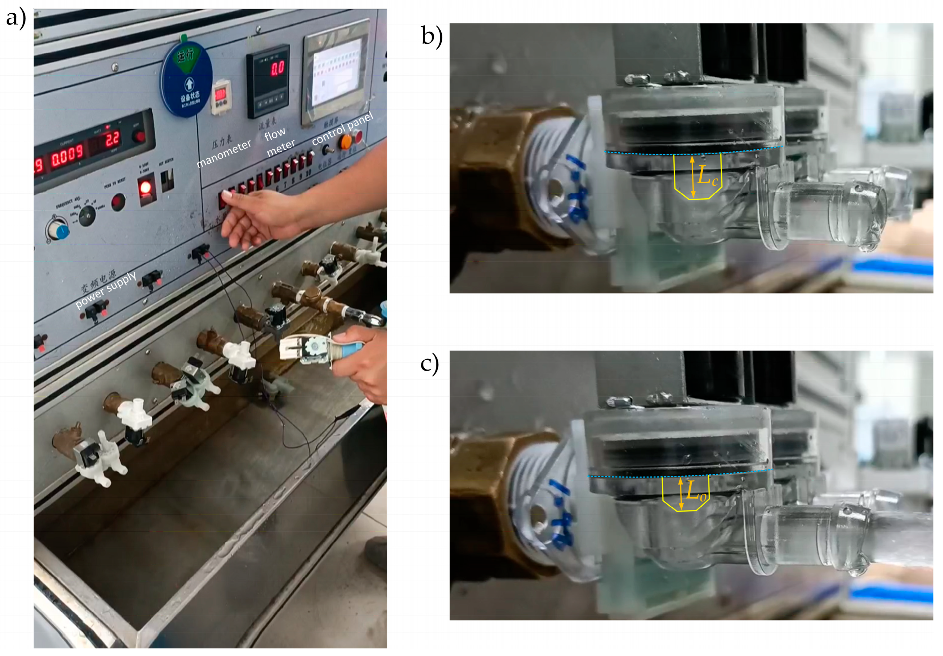
3. Experimental Setup and Procedure

An experimental study was conducted to determine the diaphragm displacement under relevant operating conditions. These conditions were selected based on the specific requirements of systems employing the previously mentioned valve design, focusing on a flow rate range at the valve inlet from 3.95 L/min to 11.9 L/min. The investigation covered several operating modes, measuring diaphragm displacement in each case for subsequent CFD modeling.

The valve model was manufactured utilizing injection molding technology using the Precision Molding 120–250 machine by KraussMaffei (Parsdorf, Germany). Polycarbonate was selected for the model due to its suitable mechanical properties, including surface purity and transparency, making it ideal for transparent prototyping.

The experimental study of valve displacement was conducted using the experimental setup model Q/HC11-033, as shown in Figure 2a. This setup was developed following several valve testing standards (including IEC 60335-1:2010 [37], GB/T 14536.9-2008 [38], QB/T 4274-2011 [39], and QB/T 1291-1991 [40]) and allows for tracking pressure drop and flow rate values at the valve inlet. The water temperature remained constant at 18.3 °C throughout the experiment.

The experiment was conducted following these steps. At first, to determine the diaphragm displacement, two high-resolution images of the valve were taken (10,120 × 5700 pixels): one in the closed position (Figure 2b) and the other in the open position (Figure 2c) under specified operating parameters. Next, a reference line, indicated by the blue dashed line in Figure 2b,c, was established on each image to measure the diaphragm length. The reference lines were selected as contour lines on the valve surface that remained unchanged regardless of its position. Additionally, the diaphragm contour (indicated by yellow lines in Figure 2b,c) was outlined, visible through the valve’s transparent walls. The diaphragm displacement ΔL was determined from the difference between the diaphragm length in the closed position L_c and the diaphragm length in the open position L_o:

ΔL = L_c − L_o.

(1)

These measurement steps were repeated 30 times for each flow regime. The average diaphragm displacement value, along with the corresponding standard error of the mean (SEM), was then calculated. The data obtained were used to create the computational domain for CFD modeling and to analyze pressure and velocity distribution inside the valve.

4. Numerical Simulation

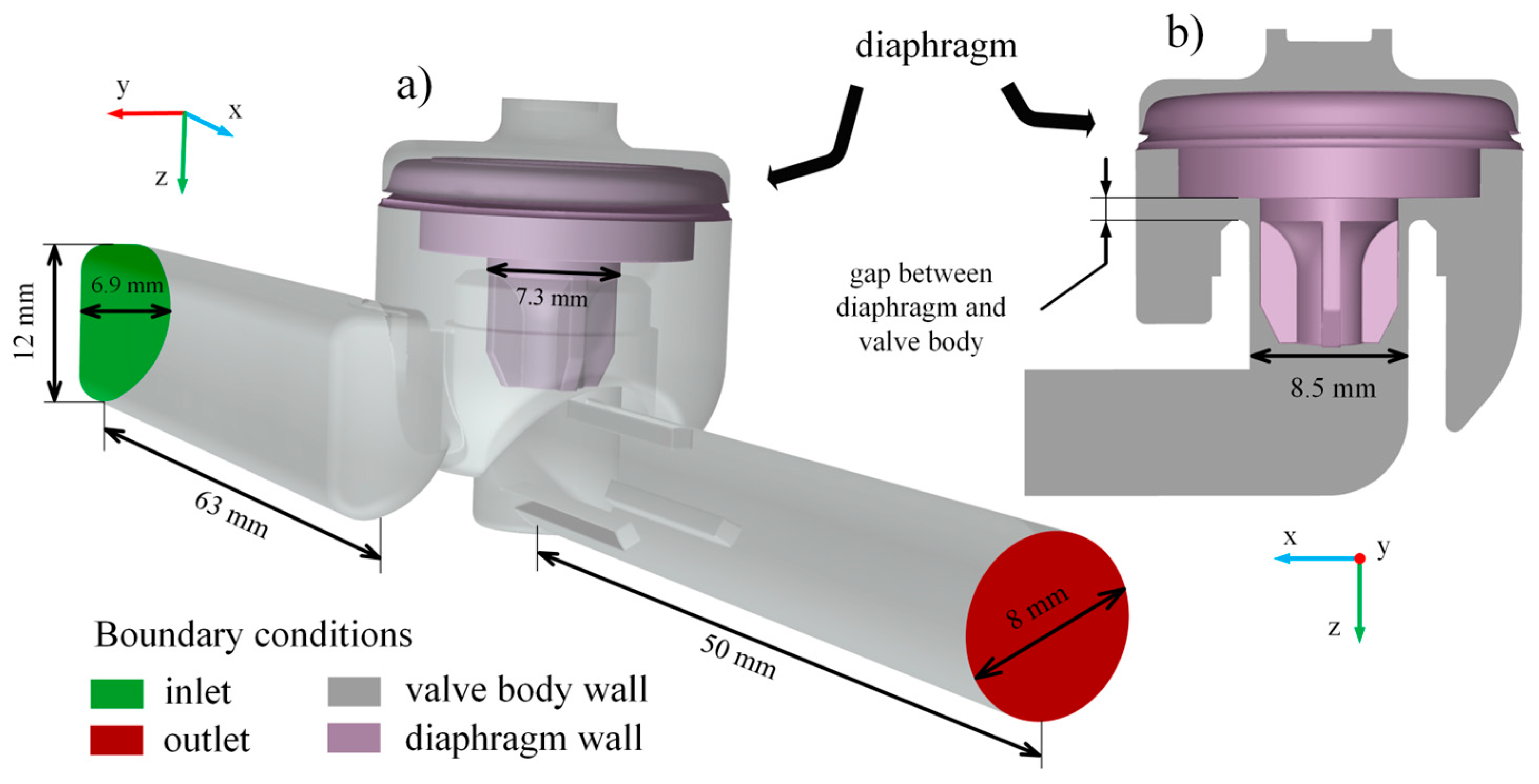
4.1. Computation Domain Boundary Conditions and Mesh

Figure 3 shows the computational domain with boundary conditions and some dimensions. The inlet and outlet boundaries were deliberately moved away from the valve’s original positions to ensure stable fluid flow at the computational domain’s inlet and outlet. Consequently, the lengths of the inlet and outlet channels were increased by approximately 5 and 6 times, respectively, compared to the diameter of the valve inlet and outlet. The volumetric flow rate of the fluid, determined during the experimental study of diaphragm displacement, was set at the inlet boundary. At the outlet boundary, atmospheric pressure was specified. The turbulence intensity I = 5% and the turbulent viscosity ratio to molecular viscosity μ_t/μ_m = 8 were set at both the inlet and outlet boundaries. A no-slip boundary condition was applied to the valve walls and the diaphragm. The main water properties specified in the simulation included a dynamic viscosity of 0.0010448 Pa⋅s and a density of 998.5 kg/m³. These parameters were based on the water temperature measured during the experiment.

The accuracy of numerical calculations depends directly on the type and quality of the mesh used. An unstructured tetrahedral mesh was selected for the simulation. A coarse mesh was applied in non-critical regions, while a finer mesh was utilized in areas such as openings in the diaphragm and the gap between the diaphragm and the valve body. This approach balances computational efficiency with accuracy, as localized refinement effectively captures flow dynamics in critical zones without significantly increasing computational costs. A mesh independence test was conducted for the valve model under maximum volumetric flow conditions of 11.9 L/min. As a result of the test (Figure 4), the number of elements was approximately 5.14 million cells, with a cell size of 0.0003 m and an average orthogonal quality of 0.861. A cell size similar to that used in the mesh independence test was selected for the other computational meshes in the investigated cases.

Since a coarse mesh is used, scalable wall functions are employed to model near-wall flow behavior. This method is well suited for turbulent simulations, balancing accuracy and computational cost. The non-dimensional distance from the wall, Y+, for all investigated cases in regions of highest velocity ranged between 39.8 and 55.2 during the numerical simulations. These values fall within the optimal range for wall functions, ensuring accurate resolution of turbulent boundary layer effects while maintaining computational efficiency.

4.2. CFD Governing Equations

To accurately model fluid flow inside the semi-direct acting solenoid valve, several assumptions were made to simplify the governing equations, ensuring computational efficiency while maintaining physical relevance. The flow was assumed to be incompressible, isothermal, and in a steady-state condition, allowing the neglect of variations in density, temperature, and time-dependent effects. Turbulence was modeled using the standard k − ϵ turbulence model due to its robustness and suitability for the relatively straightforward flow characteristics anticipated in this study.

The computational domain was idealized to represent valve geometry, and boundary conditions were carefully chosen to reflect realistic operating conditions. Additionally, material properties such as fluid density and viscosity were treated as constants, assuming a Newtonian fluid. These simplifications enabled the use of Reynolds-averaged Navier–Stokes (RANS) equations with appropriate closure for turbulent effects, providing a balance between computational efficiency and accuracy.

The continuity equation in vector form describes the conservation of mass as fluid flows through a specified space. For turbulent, incompressible, and isothermal flow under steady-state conditions, the continuity equation applied to a fixed reference frame is expressed as follows:

$$\nabla ·\mathbf{u}=0,$$

(2)

where u = [u_x, v_y, w_z]^T is the mean velocity vector, and ∇ represents the divergence operator.

The momentum equation in vector form describes the force balance on a fluid element. For incompressible flow, it is given by the following:

$$\rho \left(\mathbf{u}·\nabla \mathbf{u}\right)=-\nabla \overline{p}+\mu {\nabla }^2\mathbf{u}-\nabla ·\overline{{\mathbf{u}}^{\mathit{\prime }}{\mathbf{u}}^{\mathit{\prime }}},$$

(3)

where ρ is the fluid density (constant for incompressible flow), ρ(u⋅∇u) represents the convective term, $-\nabla \overline{p}$ is the pressure gradient force, $\mu {\nabla }^2\overline{\mathbf{u}}$ is the viscous force (with μ being the dynamic viscosity), and $-\nabla ·\overline{{\mathbf{u}}^{\mathit{\prime }}{\mathbf{u}}^{\mathit{\prime }}}$ represents the divergence of the Reynolds stress tensor, accounting for turbulent effects.

In addition to the RANS equations, the standard k − ϵ turbulence model is used, according to its wide application for valve studies [17,18,41,42], providing closure by relating the Reynolds stresses to the turbulent kinetic energy k and the dissipation rate ϵ. The k − ϵ model was deemed sufficient for the relatively simple flow characteristics expected in this study. The equation for the turbulent kinetic energy k is as follows:

$$\rho \left(\mathbf{u}·\nabla k\right)=\nabla ·\left[\left(\mu +{\displaystyle \frac{{\mu }_t}{{\sigma }_k}}\right)\nabla k\right]+P_k-\rho ϵ,$$

(4)

where the term ρ(u⋅∇k) represents the transport of turbulent kinetic energy, and k is the turbulent kinetic energy per unit mass; the term $\nabla ·\left[\left(\mu +{\displaystyle \frac{{\mu }_t}{{\sigma }_k}}\right)\nabla k\right]$ accounts for diffusion of turbulent kinetic energy, where μ, μ_t are the molecular and the turbulent (or eddy) viscosity of the fluid, respectively, σ_k is the turbulent Prandtl number for k (σ_k = 1.0); P_k is the production term of turbulent kinetic energy, typically given by the following:

$$P_k={\mu }_t\left[\left(\nabla \mathbf{u}+{\left(\nabla \mathbf{u}\right)}^T\right):\nabla \mathbf{u}\right],$$

(5)

where ∇u is the gradient of the mean velocity vector u; (∇u)^T is the transpose of the gradient of the mean velocity; : is the double dot product or Frobenius inner product.

The equation for the turbulent dissipation rate ϵ is as follows:

$$\rho \left(\mathbf{u}·\nabla ϵ\right)=\nabla ·\left[\left(\mu +{\displaystyle \frac{{\mu }_t}{{\sigma }_k}}\right)\nabla ϵ\right]+{\displaystyle \frac{ϵ}{k}}\left(C_{ϵ1}{P}_k-C_{ϵ2}ϵ\right),$$

(6)

where the term ρ(u⋅∇ϵ) represents the transport of turbulent dissipation rate, and ϵ is the turbulent dissipation rate per unit mass; the term $\nabla ·\left[\left(\mu +{\displaystyle \frac{{\mu }_t}{{\sigma }_{ϵ}}}\right)\nabla ϵ\right]$ accounts for diffusion of dissipation rate, σ_ϵ is the turbulent Prandtl number for ϵ (σ_ϵ = 1.3), and C_ϵ1 and C_ϵ2 are empirical constants (C_ϵ1 = 1.44 and C_ϵ2 = 1.92).

These equations are used to calculate the turbulent viscosity μ_t from k and ϵ as follows:

$${\mu }_t={\displaystyle \frac{C_{\mu }{k}^2}{ϵ}},$$

(7)

where C_μ is another empirical constant, which equals 0.09.

4.3. Numerical Methods

The finite volume method discretizes the computational domain into a mesh of tetrahedral control volumes, allowing for the effective resolution of the governing equations of fluid dynamics. The segregated SIMPLEC (SIMPLE-Consistent) algorithm [43] is utilized to couple the pressure and velocity fields within the liquid phase. This enhanced version of the SIMPLE algorithm improves convergence and accuracy by incorporating consistent corrections to the pressure and velocity fields. A second-order pressure discretization scheme [44] is employed to ensure that pressure gradients are accurately resolved, which is crucial for maintaining stability and improving the overall accuracy of fluid dynamics simulations, especially in flows characterized by significant pressure variations. The spatial discretization of momentum, turbulent kinetic energy, and turbulent dissipation rate variables across the tetrahedral control volumes is achieved using the second-order upwind scheme [45]. This approach enhances accuracy in capturing convective terms while minimizing numerical diffusion, which is essential for reliably simulating complex fluid dynamics. An iterative solution approach [46] is employed to solve the governing equations, with convergence deemed satisfactory when the residuals—representing the difference between the left-hand side and right-hand side of the equations—fall below a predefined threshold of 10⁻³. This criterion indicates that the solution has reached an acceptable level of accuracy and stability, reflecting reliable numerical results for key variables such as velocity, pressure, and turbulence quantities. The iterative process proceeds until the convergence criterion is satisfied, ensuring the numerical solution is both accurate and stable.

5. Results and Discussions

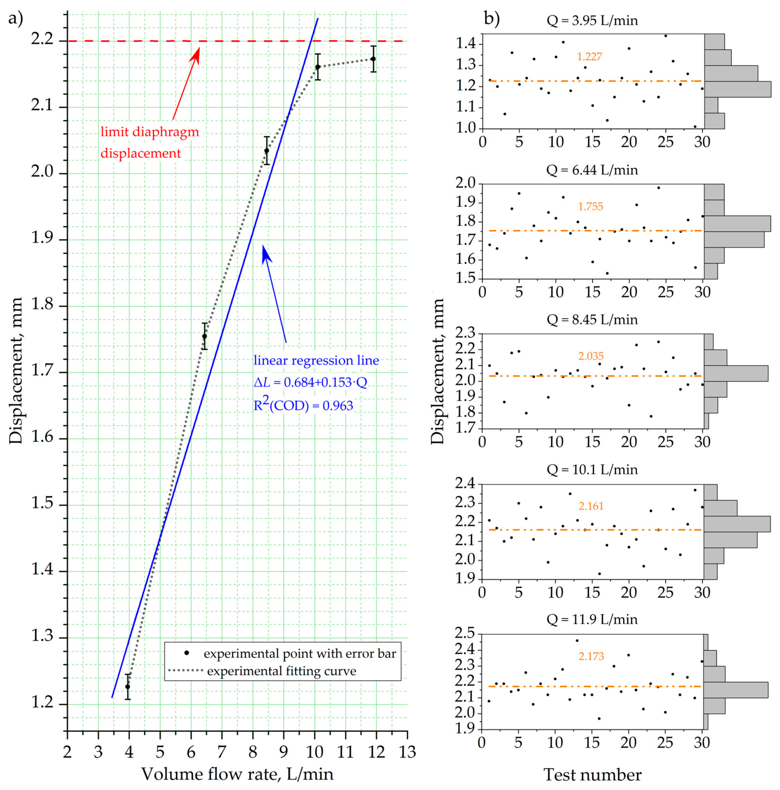
5.1. Experimental Results of Diaphragm Displacement

Based on the experimental study conducted,

Table 1. Experimental results.

Flow Rate Q, L/min	Pressure Drop ΔP (exp), kPa	Diaphragm Displacement ΔL, mm	SEM of Diaphragm Displacement
3.95	7.7	1.227	0.0189
6.44	15.1	1.755	0.0199
8.45	22.6	2.035	0.0209
10.1	32.2	2.161	0.0195
11.9	44.7	2.173	0.0196

presents the results of the pressure drop as well as the diaphragm displacement of the valve for the specified volumetric flow rate (Figure 5a). The table also includes the standard error of the mean (SEM) for diaphragm displacement, as the measurements were taken 30 times for each flow regime under investigation, and the average value (Figure 5b) was used for CFD modeling.

The graph analysis depicting the relationship between diaphragm displacement and volumetric flow rate (Figure 5a) shows that, within the flow rate range from 3.95 L/min to 10.1 L/min, the diaphragm displacement occurs linearly. It is evidenced by the linear regression line shown in Figure 5a that ΔL = 0.684 + 0.153·Q with R² = 0.963. However, with a further increase in flow rate, this relationship is disrupted, indicating that the diaphragm has reached its maximum displacement and the valve transitions into saturation mode. In this state, the valve is no longer able to compensate for the increase in flow rate, which reduces the precision of regulation and the overall system efficiency. According to the valve design, the maximum possible gap between the valve body and the diaphragm is 2.2 mm, and the experimental data presented confirm this. At a volumetric flow rate of 10.1 L/min, the diaphragm displacement is 2.161 ± 0.0195 mm. In this case, the upper surface of the diaphragm nearly touches the valve body, which explains the reduced response with further increases in volumetric flow rate up to 11.9 L/min, where the diaphragm displacement is 2.173 ± 0.0196 mm.

The experimental data presented were utilized for numerical modeling, specifically to create a more detailed computational domain that incorporates diaphragm displacement. In the proposed research framework, the sole assumption is the neglect of potential vibrations of the diaphragm caused by flow pulsations, which are deemed insignificant. This simplification enables concentration on the fundamental fluid dynamics governing the valve operation, eliminating the additional complexity associated with dynamic diaphragm behavior.

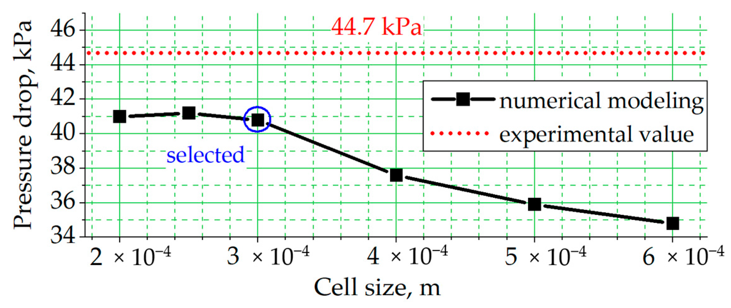
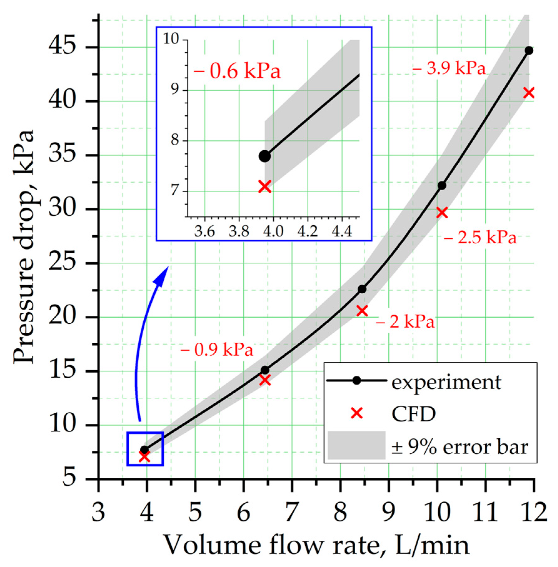
5.2. Pressure Drop Comparison and CFD Model Validation

The numerical modeling outcomes were compared with the experimental data to verify the results. The pressure drops at the inlet and outlet of the valve for specified values of water volumetric flow rates, as shown in Figure 6, were chosen as comparison parameters. As illustrated, the simulation values fall within a range of ±9% from the experimental results, indicating a high degree of agreement between the numerical calculations and the actual data. It confirms the validity of using the experimental data on diaphragm displacement, the accuracy of the chosen model, and the computational methods employed, thereby ensuring the reliability of the results for further analysis of the system parameters. The maximum error between the experiment and numerical modeling is 8.85% and is observed at a volumetric flow rate of 8.45 L/min. This maximum error indicates a reasonable level of accuracy, especially given the inherent complexities of fluid dynamics and the challenges associated with accurately capturing the behavior of the valve under varying flow conditions.

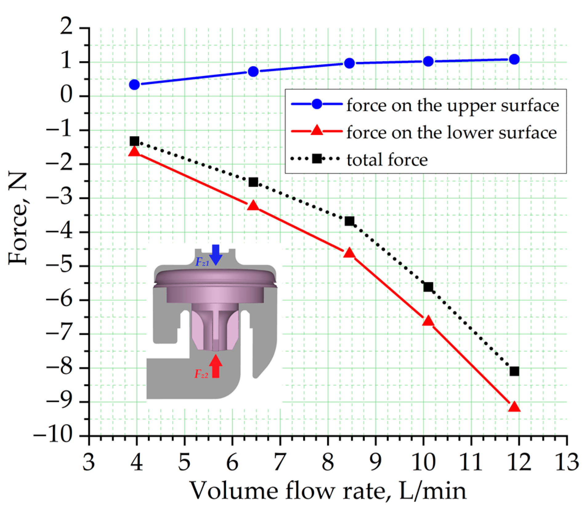
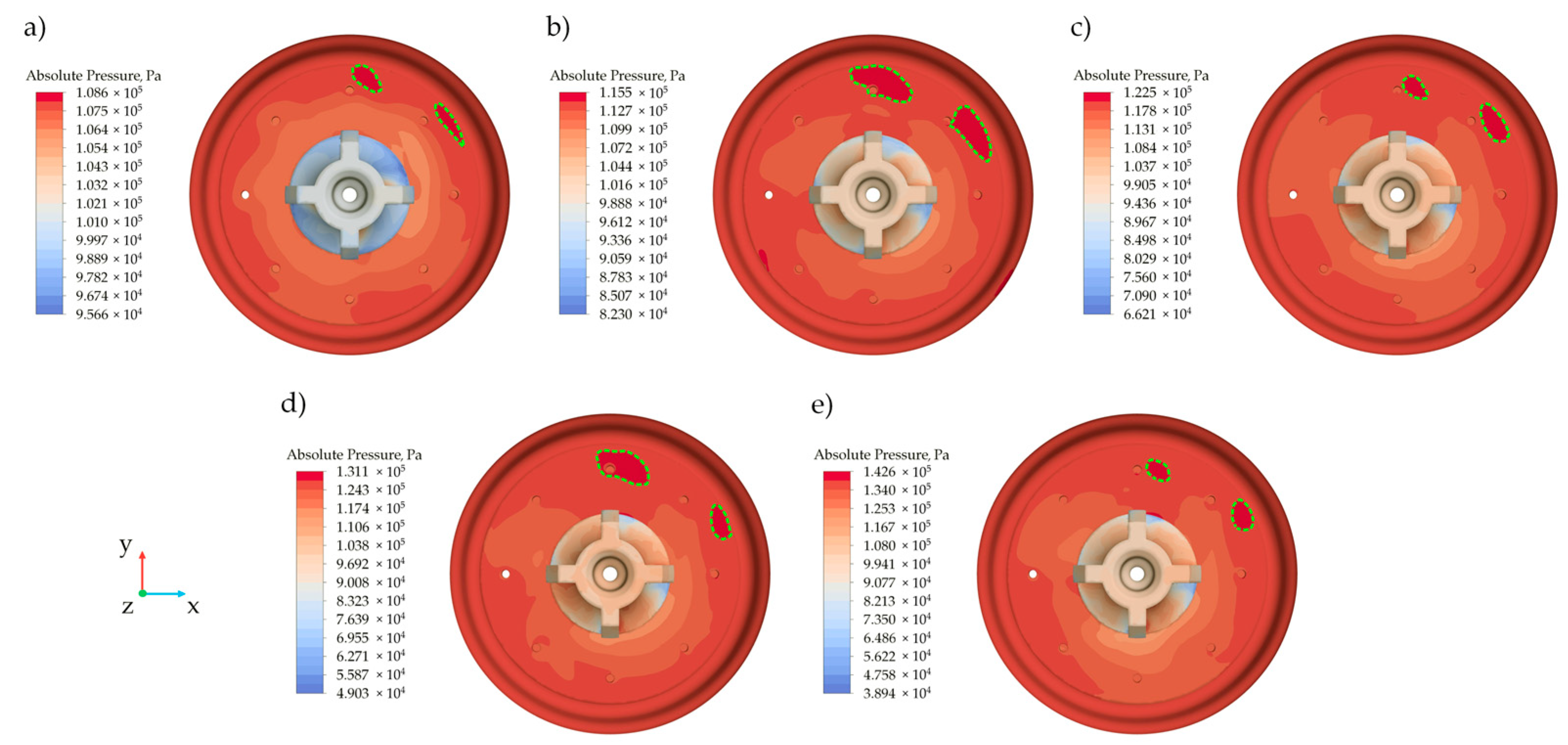
5.3. Force Action and Pressure Distribution on the Diaphragm

The pressure distribution on the diaphragm plays a crucial role in valve operation, as it directly determines the total force acting on the diaphragm. This force causes the diaphragm to move, which in turn regulates the flow of fluid through the valve.

Let us consider the total force F_z acting along the diaphragm axis, which results from the summation of the forces applied to its upper F_z1 and lower F_z2 surfaces:

$$F_z=F_{z1}-F_{z2}={\int }_{S_1}{p}_1{n}_{z1}{dA}_1-{\int }_{S_2}{p}_2{n}_{z2}{dA}_2,$$

(8)

where S₁ is the upper surface of the diaphragm, and S₂ is the lower surface; p₁ and p₂ are the pressures acting on the upper and lower surfaces, respectively; n_z1 and n_z2 are the components of the surface normals in the z-direction for the upper and lower surfaces; dA₁ and dA₂ are the elemental areas of the upper and lower surfaces, respectively. Figure 7 illustrates the relationship between the forces acting on the upper surface of the diaphragm F_z1 and the lower surface F_z2, as well as the volumetric flow rate through the valve. The figure also shows the total force F_z.

As seen in Figure 7, the force acting on the upper surface of the diaphragm is insignificant in all considered cases (several times smaller compared to the force acting on the lower surface) and does not increase significantly with the rise in volumetric flow rate. For flow rates of 3.95 L/min and 6.44 L/min, the forces acting on the upper surface of the diaphragm are 0.336 N and 0.721 N, respectively. Upon reaching a volumetric flow rate of 8.45 L/min, the force increases to 0.964 N, after which it changes little, reaching 1.023 N and 1.082 N for flow rates of 10.1 L/min and 11.9 L/min, respectively. At the same time, the force acting on the lower surface consistently increases significantly in magnitude as the volumetric flow rate increases. The total force remains negative throughout the entire range of flow rates, indicating the dominance of the force acting from below, pushing the diaphragm upward and opening the valve. At a flow rate of 8.45 L/min, the influence of the force acting on the upper surface of the diaphragm does not significantly affect the total force. Its slight variation after reaching a flow rate of 8.45 L/min indicates the onset of a critical point. It is associated with the valve’s design limitations, particularly the minimal distance between the valve body and the upper surface of the diaphragm (the upper surface of the diaphragm nearly touches the valve body, especially at flow rates of 10.1 L/min and 11.9 L/min), as was described earlier.

The analysis of pressure distribution on the lower surface of the diaphragm across all investigated regimes, as shown in Figure 8a–e, reveals a non-uniform pattern caused by the influence of water flow from the inlet channel. This occurs because the directed flow strikes the diaphragm, creating localized areas of increased pressure on its lower surface and resulting in a slightly asymmetric load. In Figure 8, the areas of maximum pressure on the diaphragm surface are highlighted with green dashed lines, maintaining a similar position relative to the center of the diaphragm in all the investigated cases. Considering the magnitude of the maximum pressure and the area it affects, it can be concluded without further calculations that the impact of the pressure is minimal and does not generate additional force that could significantly influence abnormal deflection or diaphragm stability, which was also confirmed during the experiment. However, this trend should be considered, as it indicates the potential need for valve design improvements to reduce local areas of elevated pressure and ensure a more uniform load distribution on the diaphragm.

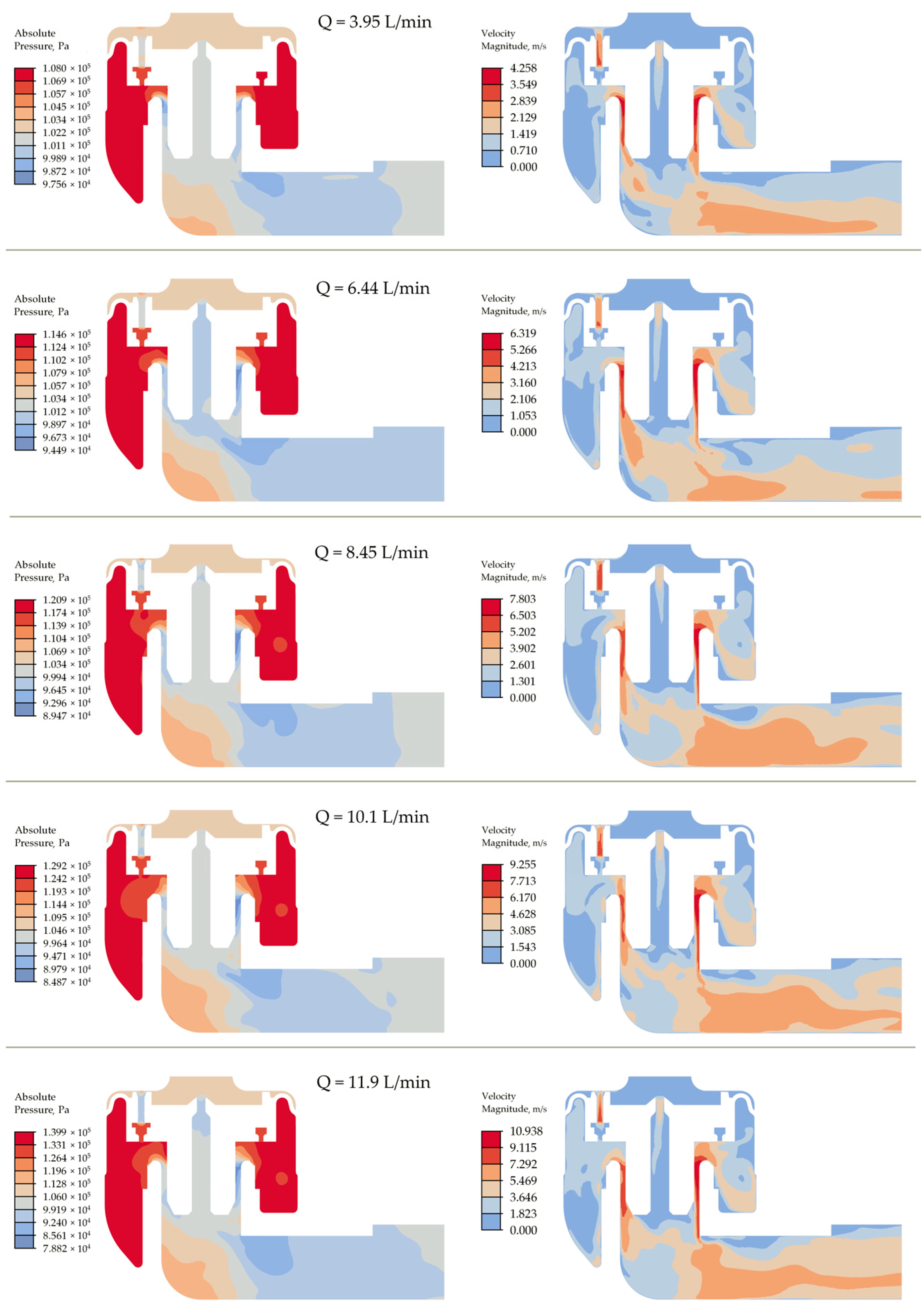
5.4. Pressure and Velocity Distribution Inside the Valve

When analyzing the pressure and velocity fields inside the valve across all the examined cases, several common patterns emerge, demonstrating how the distribution of these parameters relates to the shape of the channels and the configuration of the gaps within the valve.

In the CFD analysis of the valve design, particular attention is given to the distribution of characteristics in the sectional view passing through the axes of the diaphragm and the outlet channel. This sectional view conveys the most critical parameters influencing the valve’s operation. Figure 9 illustrates the pressure and velocity distributions in this sectional view for all investigated volumetric flow rates. In this view, key changes in pressure and flow velocity can be observed, allowing for an assessment of the flow’s interaction dynamics with valve components such as the diaphragm, valve seat, and bend at the channel turn. This distribution also plays a crucial role in evaluating the valve’s performance, flow capacity, and ability to operate stably under various working conditions.

The highest flow velocities and the corresponding minimal pressure drop are observed in the constricted areas, specifically in the gaps between the diaphragm and the valve body. The comparison of velocities in these gaps on both sides of the diaphragm demonstrates that the velocity is always higher in the gap on the right side of the diaphragm, as shown in Figure 9 and Figure 10, indicating an imbalance and a greater volumetric flow rate of water through that side. Additionally, when examining the pressure contours, it is evident that there is a more pronounced decrease in pressure on the right side of the diaphragm in the gap between the diaphragm and the valve body compared to the left side. This fluid behavior may be attributed to the design features of the valve chamber, which narrows from left to right toward the diaphragm. The narrowing of the chamber leads to increased fluid velocity on the right side of the diaphragm and the formation of vortex flow. If we examine the vector field of fluid flow in the valve chamber on the right side of the diaphragm for the lowest volumetric flow rate of 3.95 L/min, as shown in Figure 10, a well-established vortex flow is visible (vortices 1 and 2 with their directions of rotation indicated, with vortex 2 being larger in scale than vortex 1). Vortex motion is absent in the valve chamber on the left side of the diaphragm. These tendencies are characteristic of all the cases considered and become more pronounced with an increasing flow rate (with more than two vortices appearing in the area where vortices 1 and 2 are currently present).

Thus, the narrowing geometry of the valve chamber leads to dynamic changes, manifesting as an imbalance in the distribution of pressure and velocity, as well as the emergence of vortex flow, which is an undesirable effect. The drawbacks mentioned above highlight the need to optimize the design of the chamber to enhance the valve’s efficiency and improve fluid flow control. One possible solution is to make the chambers on both sides of the diaphragm equal in size or similar in size, which could help eliminate the imbalance in the distribution of pressure and velocity.

Another crucial aspect that requires attention is the channel turn from the valve chamber to the diaphragm and the outlet, as illustrated in Figure 10. The channel makes a 90-degree turn, and its inner wall features a protrusion with corner geometry, which disrupts the smoothness of the flow compared to gentle bends. Figure 10 clearly illustrates the formation of a vortex (vortex 3 with its direction of rotation indicated) after the part with corner geometry. This phenomenon represents the classical case of pressure loss caused by a change in the direction of fluid flow at a pipe bend. As seen in Figure 9, for all examined flow conditions, there is a consistent trend of pressure and velocity drop after the corner geometry. The most evident solution for optimizing the channel is to enhance flow smoothness by smoothing out the corner protrusions at the bend, which will subsequently minimize turbulence and pressure losses, thereby improving the overall efficiency of valve operation.

The final significant remark regarding the geometry of the outlet channel is the abrupt expansion of the geometry and the formation of vortex flow, as presented in Figure 10 (vortex 4 with its direction of rotation indicated). This phenomenon is a classic case of pressure losses due to the sudden expansion of the flow within the pipe. Although vortex formation has a minimal impact on the overall flow, it can be mitigated by optimizing the geometry of the outlet channel through the use of smooth transitions or rounded expansion shapes.

6. Conclusions

A combined approach was employed in this research, integrating physical prototyping with a transparent model and numerical methods to study the hydrodynamic performance of the semi-direct acting electromagnetic water valve.

The experimental study conducted led to the following conclusions:

• The analysis of diaphragm displacement as a function of volumetric flow rate in the range of 3.95–10.1 L/min showed linear behavior, confirmed by the regression equation with a high coefficient of determination.
• At a flow rate of 10.1 L/min or higher, the diaphragm reaches its maximum displacement and loses flow control accuracy, nearly touching the valve body due to a design limitation (with a maximum gap of 2.2 mm between the diaphragm surface and the valve body).
• The experiment with the transparent model enabled accurate measurement of the diaphragm displacement, forming the basis for CFD analysis. Validation showed good agreement between the calculated and experimental pressure drop data.

The numerical modeling led to the following conclusions:

• For all considered cases, the force acting on the upper surface of the diaphragm is insignificant (compared to the force on the lower surface) and changes little with increasing flow rate, reaching a maximum of 1.082 N at 11.9 L/min. At 8.45 L/min, a critical point is observed, beyond which the force on the upper surface of the diaphragm does not significantly increase with further flow rate increases due to the diaphragm reaching its maximum displacement, limited by design constraints.
• The pressure analysis on the lower surface of the diaphragm shows an uneven distribution caused by the water flow from the inlet pipe, with clearly localized areas of increased pressure. Although these zones do not affect the diaphragm’s operational stability, they indicate the need for inlet pipe optimization.
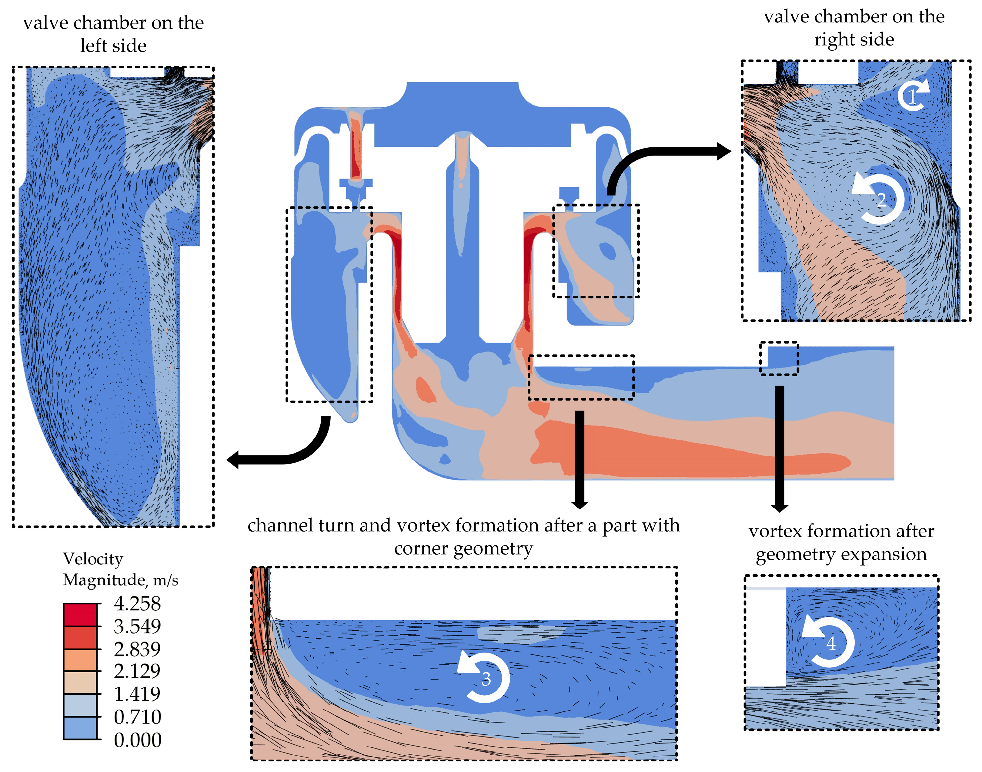
• The pressure and velocity distribution analysis in the sectional view through the diaphragm and outlet channel axes shows the higher flow capacity on the right side of the diaphragm, indicating a flow imbalance. Vortex flows are also observed in the chamber on the right side of the diaphragm. To resolve this issue, designing the valve chamber symmetrically on either side of the diaphragm is recommended.
• The analysis of the outlet channel geometry reveals that the corner protrusions on the inner wall at the channel bend and the abrupt expansion in the channel cause vortex formation and pressure losses, negatively affecting the valve efficiency. To resolve these issues, refining the channel geometry by incorporating smooth transitions and curved forms is recommended.

Future studies should build upon the current research by exploring advanced design optimization, particularly through the use of 3D CFD simulations, to capture three-dimensional flow effects and improve performance predictions under varied operating conditions. Further experimental investigations are needed to evaluate the valve’s behavior under dynamic flow conditions and in more diverse real-world scenarios. Additionally, expanding this study to include fluctuating flow rates and multiphase flows would broaden the relevance of the findings for industrial applications. These future research directions will enhance the understanding of the valve’s hydrodynamic behavior and support its optimization for a wide array of applications.

References

1. Dickenson, T.C. Valves, Piping and Pipelines Handbook, 3rd ed.; Elsevier Science Ltd.: New York, NY, USA, 1999; ISBN 978-1-85617-252-3. [Google Scholar]
2. Nesbitt, B. Handbook of Valves and Actuators: Valves Manual International; Elsevier: Amsterdam, The Netherlands, 2011; ISBN 978-0-08-054928-6. [Google Scholar]
3. Berladir, K.; Hatala, M.; Hovorun, T.; Pavlenko, I.; Ivanov, V.; Botko, F.; Gusak, O. Impact of Nitrocarburizing on Hardening of Reciprocating Compressor’s Valves. Coatings 2022, 12, 574. [Google Scholar] [CrossRef]
4. Rabie, M.G. Fluid Power Engineering, 2nd ed.; McGraw Hill: New York, NY, USA, 2023; ISBN 978-1-265-51547-8. [Google Scholar]
5. Hlubek, N.; Baumann, M.; Heinze, S.; Ostermaier, F. Using Machine Learning for Diaphragm Prediction in Solenoid Valves. In Proceedings of the 2022 IEEE 27th International Conference on Emerging Technologies and Factory Automation (ETFA), Stuttgart, Germany, 6–9 September 2022; pp. 1–4. [Google Scholar]
6. Więcławski, K.; Figlus, T.; Mączak, J.; Szczurowski, K. Method of Fuel Injector Diagnosis Based on Analysis of Current Quantities. Sensors 2022, 22, 6735. [Google Scholar] [CrossRef] [PubMed]
7. Duan, Z.; Jia, Y.; Ren, X.; Jiang, H.; Lv, Y.; Song, H.; Chen, H.; Zhai, H. Analysis of Fluid-Structure Interaction in Diaphragm Plug Valves for Filling Electrolyte in Lithium-Ion Battery Cells. Flow Meas. Instrum. 2024, 98, 102632. [Google Scholar] [CrossRef]
8. Ye, P.; Zhang, C. Flow Field Analysis and Flow Prediction of Pressure Reducing Valves in Power-Law Media. Flow Meas. Instrum. 2024, 99, 102657. [Google Scholar] [CrossRef]
9. Demir, U.; Coskun, G.; Soyhan, H.S.; Turkcan, A.; Alptekin, E.; Canakci, M. Effects of Variable Valve Timing on the Air Flow Parameters in an Electromechanical Valve Mechanism—A Cfd Study. Fuel 2022, 308, 121956. [Google Scholar] [CrossRef]
10. Han, J.; Xie, Y.; Wang, Y.; Wang, Q.; Zhang, Y.; Ju, J. Research on Dynamicflow Rate Self-Sensing in Control Valves. Prog. Nucl. Energy 2024, 176, 105377. [Google Scholar] [CrossRef]
11. Cao, L.; Liu, S.; Hu, P.; Si, H. The Influence of Governing Valve Opening on the Erosion Characteristics of Solid Particle in Steam Turbine. Eng. Fail. Anal. 2020, 118, 104929. [Google Scholar] [CrossRef]
12. Wen, Q.; Liu, Y.; Chen, Z.; Wang, W. Numerical Simulation and Experimental Validation of Flow Characteristics for a Butterfly Check Valve in Small Modular Reactor. Nucl. Eng. Des. 2022, 391, 111732. [Google Scholar] [CrossRef]
13. Xie, C.; Su, H.; Yang, J.; He, Z. Design and Analysis of Combined Valve Spool with Linear Flow Coefficient. J. Eng. 2022, 2022, 6006810. [Google Scholar] [CrossRef]
14. Qu, Q.; Wang, L.; Chen, H.; Dai, N.; Jia, P.; Xu, D.; Li, L. Study on Flow Characteristics of the Cryogenic Throttle Valve for Superfluid Helium System. Cryogenics 2024, 138, 103797. [Google Scholar] [CrossRef]
15. Ledvoň, M.; Hružík, L.; Bureček, A.; Polášek, T.; Dýrr, F.; Kolář, D. Experimental and Numerical Analysis of Flow Force Acting on the Spool of Proportional Directional Valve. Processes 2023, 11, 3415. [Google Scholar] [CrossRef]
16. Li, Q.; Zong, C.; Liu, F.; Zhang, A.; Xue, T.; Yu, X.; Song, X. Numerical and Experimental Analysis of Fluid Force for Nuclear Valve. Int. J. Mech. Sci. 2023, 241, 107939. [Google Scholar] [CrossRef]
17. Filo, G.; Lisowski, E.; Rajda, J. Pressure Loss Reduction in an Innovative Directional Poppet Control Valve. Energies 2020, 13, 3149. [Google Scholar] [CrossRef]
18. Filo, G.; Lisowski, E.; Rajda, J. Design and Flow Analysis of an Adjustable Check Valve by Means of CFD Method. Energies 2021, 14, 2237. [Google Scholar] [CrossRef]
19. Shu, Z.; Liang, W.; Qin, B.; Lei, G.; Wang, T.; Huang, L.; Che, B.; Zheng, X.; Qian, H. Transient Flow Dynamics Behaviors during Quick Shut-off of Ball Valves in Liquid Hydrogen Pipelines and Storage Systems. J. Energy Storage 2023, 73, 109049. [Google Scholar] [CrossRef]
20. Gao, H.; Mo, Y.; Wu, F.; Wang, J.; Gong, S. Impact of Elastic Diaphragm Hardness and Structural Parameters on the Hydraulic Performance of Automatic Flushing Valve. Water 2023, 15, 287. [Google Scholar] [CrossRef]
21. Shamsi, A.; Mazloum, J. Numerical Study of a Membrane-Type Micro Check-Valve for Microfluidic Applications. Microsyst. Technol. 2020, 26, 367–376. [Google Scholar] [CrossRef]
22. Lin, Z.; Li, X.; Jin, Z.; Qian, J. Fluid-Structure Interaction Analysis on Membrane Behavior of a Microfluidic Passive Valve. Membranes 2020, 10, 300. [Google Scholar] [CrossRef]
23. Wu, W.; Guo, T.; Peng, C.; Li, X.; Li, X.; Zhang, Z.; Xu, L.; He, Z. FSI Simulation of the Suction Valve on the Piston for Reciprocating Compressors. Int. J. Refrig. 2022, 137, 14–21. [Google Scholar] [CrossRef]
24. Domagala, M.; Fabis-Domagala, J. A Review of the CFD Method in the Modeling of Flow Forces. Energies 2023, 16, 6059. [Google Scholar] [CrossRef]
25. Lin, Z.; Hou, C.; Zhang, L.; Guan, A.; Jin, Z.; Qian, J. Fluid-Structure Interaction Analysis on Vibration Characteristics of Sleeve Control Valve. Ann. Nucl. Energy 2023, 181, 109579. [Google Scholar] [CrossRef]
26. Xie, J.; Zeng, W.; Pan, X.; Chen, J.; Ye, J. FSI Investigation on the Discharge Valve Lift in a R32 Rotary Compressor and Its Verification. Case Stud. Therm. Eng. 2024, 61, 105108. [Google Scholar] [CrossRef]
27. Olivetti, M.; Monterosso, F.G.; Marinaro, G.; Frosina, E.; Mazzei, P. Valve Geometry and Flow Optimization through an Automated DOE Approach. Fluids 2020, 5, 17. [Google Scholar] [CrossRef]
28. Rulli, F.; Barbato, A.; Fontanesi, S.; d’Adamo, A. Large Eddy Simulation Analysis of the Turbulent Flow in an Optically Accessible Internal Combustion Engine Using the Overset Mesh Technique. Int. J. Engine Res. 2021, 22, 1440–1456. [Google Scholar] [CrossRef]
29. Bornoff, J.; Gill, H.S.; Najar, A.; Perkins, I.L.; Cookson, A.N.; Fraser, K.H. Overset Meshing in Combination with Novel Blended Weak-Strong Fluid-Structure Interactions for Simulations of a Translating Valve in Series with a Second Valve. Comput. Methods Biomech. Biomed. Eng. 2024, 27, 736–750. [Google Scholar] [CrossRef]
30. Kim, N.-S.; Jeong, Y.-H. An Investigation of Pressure Build-up Effects Due to Check Valve’s Closing Characteristics Using Dynamic Mesh Techniques of CFD. Ann. Nucl. Energy 2021, 152, 107996. [Google Scholar] [CrossRef]
31. Neyestanaki, M.K.; Dunca, G.; Jonsson, P.; Cervantes, M.J. A Comparison of Different Methods for Modelling Water Hammer Valve Closure with CFD. Water 2023, 15, 1510. [Google Scholar] [CrossRef]
32. Yao, H.; Ye, Q.; Wang, C.; Yuan, P. CFD Dynamic Mesh-Based Simulation and Performance Investigation of Combined Guided Float Valve Tray. Chem. Eng. Process. -Process Intensif. 2023, 193, 109523. [Google Scholar] [CrossRef]
33. Rogovyi, A.; Korohodskyi, V.; Medvediev, Y. Influence of Bingham Fluid Viscosity on Energy Performances of a Vortex Chamber Pump. Energy 2021, 218, 119432. [Google Scholar] [CrossRef]
34. Li, Y.; Zhou, H.; Liu, H.; Ding, X.; Zhang, W. Geotechnical Properties of 3D-Printed Transparent Granular Soil. Acta Geotech. 2021, 16, 1789–1800. [Google Scholar] [CrossRef]
35. Nilsson, D.P.G.; Holmgren, M.; Holmlund, P.; Wåhlin, A.; Eklund, A.; Dahlberg, T.; Wiklund, K.; Andersson, M. Patient-Specific Brain Arteries Molded as a Flexible Phantom Model Using 3D Printed Water-Soluble Resin. Sci. Rep. 2022, 12, 10172. [Google Scholar] [CrossRef] [PubMed]
36. Ju, Y.; Gong, W.; Zheng, J. Effects of Pore Topology on Immiscible Fluid Displacement: Pore-Scale Lattice Boltzmann Modelling and Experiments Using Transparent 3D Printed Models. Int. J. Multiph. Flow 2022, 152, 104085. [Google Scholar] [CrossRef]
37. 60335-1:2010; Household and similar electrical appliances-Safety-Part 1: General requirements. International Electrotechnical Commission: Geneva, Switzerland, 2010.
38. GB 14536.9-2008; Automatic electrical controls for household and similar use - Particular requirements for electrically operated water valves, including mechanical requirements. China Standard Publishing House: Beijing, China, 2008.
39. QB/T 4274-2011; Technical conditions for inlet valve of washing machine. China Standard Publishing House: Beijing, China, 2011.
40. QB/T 1291-1991; Water inletting electromagnetic valves intended to be used in automatic washing machines. China Standard Publishing House: Beijing, China, 1991.
41. Zhu, G.; Dong, S.M. Analysis on the Performance Improvement of Reciprocating Pump with Variable Stiffness Valve Using CFD. J. Appl. Fluid Mech. 2020, 13, 387–400. [Google Scholar] [CrossRef]
42. Wu, W.; Qiu, B.; Tian, G.; Liao, X.; Wang, T. CFD-Based Cavitation Research and Structure Optimization of Relief Valve for Noise Reduction. IEEE Access 2022, 10, 66356–66373. [Google Scholar] [CrossRef]
43. Patankar, S.V. Numerical Heat Transfer and Fluid Flow; CRC Press: Boca Raton, FL, USA, 2018; ISBN 978-1-315-27513-0. [Google Scholar]
44. Ferziger, J.H.; Peric, M. Computational Methods for Fluid Dynamics, 3rd ed.; Springer: Berlin/Heidelberg, Germany, 2002; ISBN 978-3-642-56026-2. [Google Scholar]
45. LeVeque, R.J. Finite Volume Methods for Hyperbolic Problems; Cambridge Texts in Applied Mathematics; Cambridge University Press: Cambridge, UK, 2002; ISBN 978-0-521-00924-9. [Google Scholar]
46. Smith, G.D. Numerical Solution of Partial Differential Equations: Finite Difference Methods, 3rd ed.; Clarendon Press: Oxford, UK, 1986; ISBN 978-0-19-859650-9. [Google Scholar]
Figure 1. Illustration of the real valve (a); closed position of the valve (b); and open position of the valve (c).
Water 16 03385 g001
Figure 2. Experimental setup (a); closed position of the valve (b); and open position of the valve (c).
Water 16 03385 g002
Figure 3. Computational domain and boundary conditions: the entire valve (a) and sectional view (b).
Water 16 03385 g003
Figure 4. Mesh independence test results.
Water 16 03385 g004
Figure 5. Experimental results of the relationship between diaphragm displacement and volumetric flow rate (a) and determination of the average diaphragm displacement for each investigated volumetric flow rate (b).
Water 16 03385 g005
Figure 6. Comparison of pressure drop across the valve: experiment versus CFD.
Water 16 03385 g006
Figure 7. Forces acting on the diaphragm: comparison of forces on the upper and lower surfaces, and the resulting total force across the range of volumetric flow rates.
Water 16 03385 g007
Figure 8. Pressure distribution on the lower surface of the diaphragm at different flow rates: 3.95 L/min (a), 6.44 L/min (b), 8.45 L/min (c), 10.1 L/min (d), 11.9 L/min (e).
Water 16 03385 g008
Figure 9. Pressure and velocity distribution.
Water 16 03385 g009
Figure 10. Contours and vector field of velocities for the case with a volumetric flow rate of 3.95 L/min.
Water 16 03385 g010