Abstract
Amidst changing climatic conditions, accurately predicting reservoir inflows in an extreme event is challenging and inevitable for reservoir management. This study proposed an innovative strategy under such circumstances through rigorous experimentation and investigations using 18 years of monthly data collected from the Huai Nam Sai reservoir in the southern region of Thailand. The study employed a two-step approach: (1) isolating extreme and normal events using quantile regression (QR) at the 75th, 80th, and 90th quantiles and (2) comparing the forecasting performance of individual machine learning models and their combinations, including Random Forest (RF), eXtreme Gradient Boosting (XGBoost), Long Short-Term Memory (LSTM), and Multiple Linear Regression (MLR). Forecasting accuracy was assessed at four lead times—3, 6, 9, and 12 months—using ten-fold cross-validation, resulting in 16 model configurations for each forecast period. The results show that combining quantile regression (QR) to distinguish between extreme and normal events with hybrid models significantly improves the accuracy of monthly reservoir inflow forecasting, except for the 9-month lead time, where the XG model continues to deliver the best performance. The top-performing models, based on normalized scores for 3-, 6-, 9-, and 12-month-ahead forecasts, are XG-MLR-75, RF-XG-80, XG-75, and XG-RF-75, respectively. Another crucial finding of this research is the uneven decline in prediction accuracy as lead time increases. Notably, the model performed best at t + 9, followed by t + 3, t + 12, and t + 6, respectively. This pattern is influenced by model characteristics, error propagation, temporal variability, data dynamics, and seasonal effects. Improving the accuracy and efficiency of hybrid model forecasting can greatly enhance hydrological operational planning and management.
1. Introduction
Climate change and rapid population growth have sharply increased water demand, raising critical concerns for water resource management, especially during natural disasters such as earthquakes, heavy rainfall, hurricanes, and floods [1,2]. These extreme events cause rapid shifts in temperature, water levels, and rainfall, impacting hydrology by altering precipitation, inflow, streamflow, and groundwater levels. This leads to more frequent floods and droughts, affecting ecosystems and water resources [3,4,5,6]. Climate models forecast intensified rainfall, worsening flood and drought risks, especially in low-income, urbanizing regions [7,8]. In Thailand, the Twelfth National Economic and Social Development Plan (2017–2021) prioritizes water management, with the Royal Irrigation Department overseeing reservoirs to balance hydrological needs with environmental and socioeconomic demands [9]. Effective reservoir operation (RO) requires understanding the water balance (inflow, outflow, storage), which is vital to managing water resources during extreme events and minimizing potential damage across sectors [10]. Comprehensive hydrological data are essential for water management agencies to make informed decisions.
Reservoir inflow forecasting methods generally fall into three categories. First, hydrological models, like SWAT used by Tongsiri et al. [11], employ mathematical frameworks to analyze rainfall–outflow relationships in reservoirs. Second, time series models, statistical methods that predict reservoir inflow volume, have been widely applied over the last decade with techniques like ARMA, ARIMA, ARMAX, and SARIMA for monthly predictions [12,13,14,15,16]. Lastly, machine learning algorithms, including SVR, RF, and MLP, leverage historical data to enhance inflow forecasts and are extensively used in the literature [14,17,18].
To effectively manage water resources, accurately predicting reservoir inflow is essential, as it influences flood control, water supply, and hydropower capacity [19]. Factors like the El Niño-Southern Oscillation (ENSO), Southern Oscillation Index (SOI), and Dipole Mode Index (DMI) significantly affect reservoir inflow forecasts by altering precipitation patterns and intensity [20]. A major challenge in reservoir inflow forecasting, particularly in underdeveloped and developing countries, is the lack of historical data, which often compels researchers to rely on limited temporal datasets for monthly or yearly forecasts. Utilizing available historical data is crucial for predicting values necessary to address various time-series problems [21,22,23]. Integrating climate indices into machine learning models has proven valuable for reservoir inflow forecasting and operation planning. Lin et al. (2010) demonstrated improved long-term inflow predictions with SVM-based models using typhoon characteristics over BPN models [24]. Lee et al. developed a statistical ensemble model for monthly inflow at the Soyang River Dam, finding Bayesian model averaging (BMA) more accurate than simple model averaging (SMA) or naïve forecasting (NF) using fourteen meteorological features, including ENSO and SOI [25]. Yang et al. [10] showed that among SVR, RF, and ANN models, RF performed best for one-month-ahead predictions in China and the USA, especially when using NINO indices. Li et al. [22] found RF to outperform ANN, SVR, and linear models for daily inflow in China, achieving an RMSE of 0.25 m using prior week water levels from multiple stations. Although advancements have been made, few studies address inflow predictions across different lead times [17,22], underscoring the importance of FS to enhance model accuracy [23,24,25,26].
FS reduces computation time and enhances prediction accuracy by identifying the most predictive fields in a dataset, with applications in hydrology for reservoir inflow prediction [27]. FS methods include model-free techniques, like correlation-based selection, and model-based approaches that use specific search criteria. Genetic Algorithm (GA) is a prominent FS method based on natural selection, proven by Alquraish et al. [27] to improve SVM and ANFIS model accuracy for inflow forecasting. Makridakis et al. [28] advanced FS by combining sequence forward search with the LW index (SFS-LW) for cross-validation. Recent studies emphasize hybrid FS and hyperparameter tuning; for example, Cheng et al. [29] applied SVM-GA and ANN-GA, while Bai et al. [30] used multiscale deep feature learning (MDFL) for daily inflow predictions. Weekaew et al. [31] showed that Bayesian Estimation (BE) and GA were highly effective for multi-step predictions, with BE outperforming GA but with higher computational demands [12].
Direct multi-step inflow forecasting is crucial for water resource management and reservoir operations, requiring accurate time-series predictions [32]. Models like Long Short-Term Memory (LSTM) networks, gradient-boosting regression trees (GBRT), and maximal information coefficients (MIC) have been explored to improve forecasting accuracy, especially with limited data [32,33]. Stepwise prediction techniques help determine the impact of current time steps on future ones, aiding in fields such as agriculture, stock market trends, traffic, and electricity. This approach provides insights into value patterns, magnitudes, and timing for events like crop cycles, temperature ranges, and water inflows. Tabari [34] developed a hybrid model using the ERA-Interim Reanalysis dataset (2011–2018) for daily reservoir inflow, combining GBRT with MIC for predictor selection and PACF/CCF to identify inflow and rainfall lags, thereby enhancing forecast accuracy across 4- to 10-day lead times [33].
Hybrid models have become popular for complex predictions. Alquraish et al. [28], in 2021, assessed a hidden Markov model (HMM) and two hybrid models—support vector machine-genetic algorithm (SVM-GA) and artificial neural fuzzy inference system-genetic algorithm (ANFIS-GA)—for forecasting inflow at the King Fahd Dam in Saudi Arabia. They found GA improved ANFIS and SVR predictions, reducing RMSE by 25% and increasing Nash–Sutcliffe efficiency (NSE) by 13%. However, these studies did not include climatic indicators. Zheng et al. [35] introduced a multi-model fusion for reservoir inflow prediction in the Jinshuitan River Basin, combining CNN, XGBoost, and PLS to improve accuracy. Their model, tailored with loss functions for high-flow scenarios, achieved a 41.64–72.29% RMSE reduction over single models, though primarily effective for high flows, especially using XGBoost and CNN.
Research on reservoir inflow forecasting during extreme events has yielded significant findings. Yang et al. [36] demonstrated in 2014 that ensemble-mean precipitation forecasts, combined with hydrological models, reduced uncertainty in 3-day inflow predictions at Taiwan’s Shihmen Reservoir, although shorter cumulative forecasts had greater uncertainty. In 2018, Amnatsan et al. [37] found the variation analog method (VAM) most effective for extreme inflow conditions, while the wavelet artificial neural network (WANN) better predicted annual inflow trends. Huang et al. [38] evaluated seven machine learning and two ensemble techniques in 2021 for 1, 4, and 6 h lead forecasts, finding the Switched Prediction Method (SP) improved stability and accuracy for extreme events, though physical models remained computationally demanding yet effective. Chen et al. [39], in 2022, introduced a resampling approach to address imbalanced time series, grouping predictors and outputs into extreme and normal event blocks. This method, using Box–Cox transformation and deep neural networks, significantly improved forecast accuracy and was valuable for direct multi-step inflow forecasting during extreme events.
This study aims to bridge the knowledge gap by proposing a unique methodological framework that enhances the predictive ability of reservoir inflow forecasting during extreme events. Quantile regression (QR) is introduced to distinguish between extreme and normal events, and various hybrid machine learning models are developed and evaluated for forecasting reservoir inflow separately during these events. Their performance is compared with each other and with traditional individual machine learning models. The remainder of this article is organized as follows: Section 2 describes the study area and data collection and provides a brief overview of the theories used. Section 3 details the research methodology, including the research framework, experimental setup, and statistical performance measures. Section 4 presents the experimental results and subsequent discussion. Finally, the research findings are concluded in Section 5.
2. Study Area, Data Collection, and Brief Overview of Theories Used
2.1. Study Area
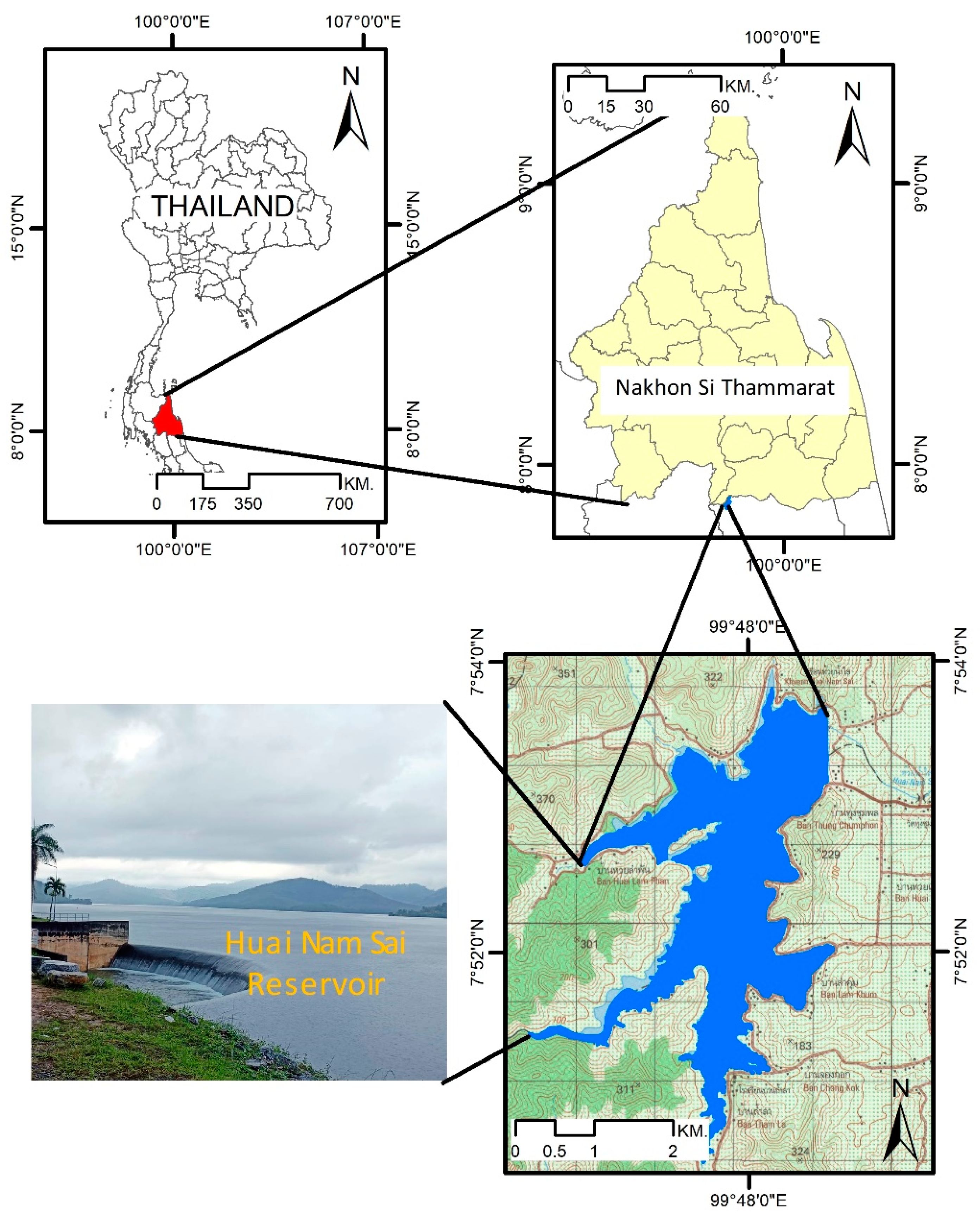
Huai Nam Sai Reservoir is located at 7°53′33.49″ N latitude and 99°48′32.43″ E longitude in Cha-uat District, Nakhon Si Thammarat province in southern Thailand. It is characterized by its moderate size. This specific reservoir is particularly susceptible to the extensive effects of climate change. Recent studies have shown a warming trend of 1.4 °C from 1851 to 2017 in Nakhon Si Thammarat. The reservoir experiences influence from northeast and southwest monsoon winds within a tropical climate, as shown in Figure 1. Serving as a prototype for the study of similar reservoirs, Huai Nam Sai was constructed in 1992 by the Royal Irrigation Department (RID). The dam of the reservoir boasts an embankment that is 8.00 m wide, 946 m long, and 40 m high.
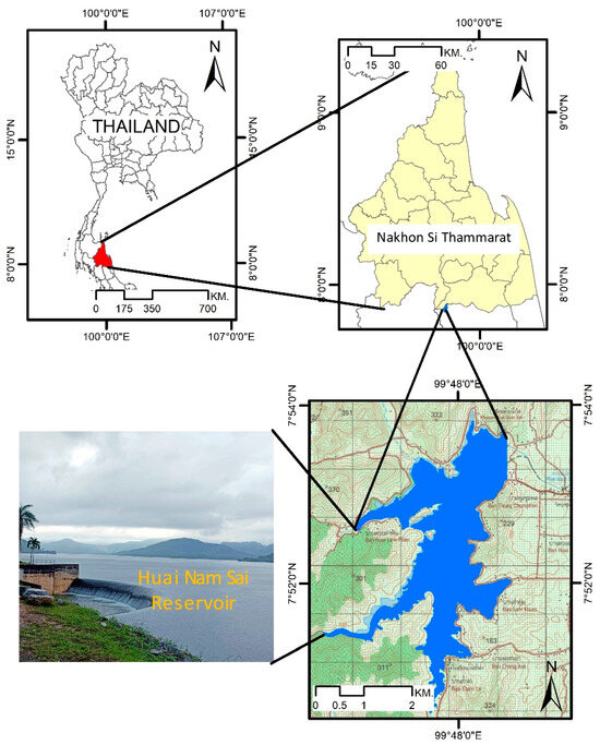
Figure 1.
The location of Huai Nam Sai Reservoir.
Presently, the Upper Pak Phanang Irrigation and Maintenance Project, under the management of Irrigation Office 15, is responsible for its operation. This essential water source plays a crucial role in supporting irrigation for a vast expanse of land, benefiting both agriculture and various industries in the region. Moreover, the reservoir contributes significantly to flood prevention efforts and sustains the local ecosystem. Its functions include improving crop productivity, cultivating off-season crops, producing rice, and facilitating fish breeding activities in the Pak Phanang area of Nakhon Si Thammarat, Thailand.
2.2. Data Collection
This research collected monthly data from 216 datasets, covering hydrological information, oceanic indices, and sea surface temperatures from 1998 to 2015, obtained from three specified sources. These sources consist of the Upper Pak Phanang Operation and Maintenance Project, managed by Irrigation Office 15 of the Royal Irrigation Department in Thailand, the Japan Agency for Marine-Earth Science and Technology (JAMSTEC), and the US National Oceanic and Atmospheric Administration (NOAA), as illustrated in Table 1.

Table 1.
The information of the data used, features, and data sources.
Numerous studies indicated that hydrological data and climate change indices are affected by accurately predicting reservoir inflow [11,12,13,14,15,16,17,18,19,20,21,22,23,24,25,26]. The relevant statistical figures are available in Table 2. The monthly dataset on reservoir hydrology includes rainfall (R) in mm/month and reservoir inflow (Inf) in m3/month. NOAA and JAMSTEC provide data on ocean indices and sea surface temperature (SST). SST can be approximated using eight input variables: NINO1+2, ANOM1+2, NINO3, ANOM3, NINO4, ANOM4, NO3.4, and ANOM3.4. There are two sources for historical climate change indicators, namely the Dipole Mode Index (DMI) and the Southern Oscillation Index (SOI). These are two oceanic indices associated with the El Niño and La Niña seasons in the Pacific Ocean. Furthermore, SST reflects the temperature of the uppermost layer of the ocean (see Table 1.). The dataset comprises 144 features of hydrological data, oceanic indices, and sea surface temperatures with the 12-month lag time series (T − 1 to T − 12). These data were utilized to forecast future reservoir inflow for 3, 6, 9, and 12 months ahead. The fundamental statistical analysis, encompassing the maximum, minimum, mean, standard deviation, kurtosis, and skewness of the data employed in this study, is outlined in Table 2.
Table 2.
The statistical examination of the used data adapted from [26].
2.3. Brief Overview of Theories Used
2.3.1. Quantile Regression
Quantile regression (QR), a statistical method developed by Koenker and Bassett in 1978 [40], enhances the classical linear regression model by estimating the conditional median or other quantiles of the response variable. This provides a more thorough examination of the relationship between variables at different points in the distribution. Unlike mean regression, which focuses only on the conditional mean, QR models the conditional quantile, enabling the exploration of how covariates impact distribution tails. This is particularly beneficial for understanding an extreme event.
In the realm of water resource management, QR can be extremely useful. It allows for the modeling of inflow distribution under various conditions rather than just forecasting average inflows. Knowing the likelihood of extreme inflow events (such as floods or droughts) can help in devising more effective planning and risk management strategies. By utilizing QR, forecasters can more effectively evaluate the risks associated with different inflow scenarios, leading to enhanced reservoir operation and preparedness for extreme conditions. Experts can better evaluate the risks associated with various inflow scenarios, leading to enhanced reservoir operation and readiness for extreme conditions. In this study, a quantile regression equation was applied to isolate extreme events from the experimental data. The QR model, designed to predict the τ-th quantile of the dependent variable y based on independent variables x1, x2,…, xn, minimizes an alternative loss function for a given quantile τ between 0 and 1. It can be mathematically written as Equation (1):
Qy(τ∣x) = β0(τ) + β1(τ)x1 + β2(τ)x2 + … + βn(τ)xn
Qy(τ∣x) represents the τ-th quantile of y given x, while β0(τ), β1(τ),…, βn(τ) correspond to the coefficients for the τ-th quantile, which differ from those used in the mean regression (OLS), and x1, x2,…, xn are the independent variables. The objective function for QR, which requires minimization, is defined as Equation (2).
∑yi < Qy(τ∣xi)τ∣yi − Qy(τ∣xi)∣ + ∑yi ≥ Qy(τ∣xi)(1 − τ)∣yi − Qy(τ∣xi)
This objective function is a weighted sum of absolute deviations, with the weights being τ for data points below the τ-th quantile and 1 − τ for data points above it. This methodology ensures the robustness of the regression model against outliers and facilitates a more comprehensive understanding of the relationship between variables by examining various segments of the response variable distribution [41,42,43]. Quantiles such as 0.05, 0.25, 0.75, and 0.95 were employed in the study to detect extreme occurrences, aligning with prior studies that yielded favorable experimental outcomes [44,45,46]. The goal of the research is to find solutions to the flooding issue. Therefore, this study employs quantile data with a minimum value of 0.75.
2.3.2. Tree-Based Machine Learning Techniques
Random Forest (RF)
The random forest (RF) algorithm selectively focuses on a subset of attributes within the training set to determine splitting nodes in decision trees. This randomization occurs at two distinct levels to enhance generalization error reduction: the selection of training records and the selection of attributes within each base classifier. In the process of building a model through bagging, a specific subset of training records is considered in each iteration. The approach of RF is founded on a similar principle to that of bagging, as described by Kotu and Deshpande in 2015 [44].
In 2001, the concept of RF was initially introduced by Leo Breiman and Adele Cutler [45]. This method is categorized as an ensemble learning technique utilized for tasks like classification and regression. The process of building a model consists of two key phases. RF produces multiple distinct trees within the decision tree framework. For each instance, two-thirds of the data is randomly chosen to construct the decision tree and compute the prediction error, while the remaining one-third is set aside as an out-of-bag error (OOB) instance. Model predictions are made using a voting strategy, where regression problems involve averaging values and classification tasks involve voting based on the predictive performance of each tree. RF is an ensemble learning approach suitable for both regression and classification purposes. It generates multiple decision trees during training and, in regression scenarios, offers the average prediction from each tree. RF’s effectiveness lies in its capacity to manage high-dimensional data, provide varied significance assessments, and prevent overfitting through ensemble methodologies. Unlike the M5 model tree (M5), mature RF trees in the M5 model are left unpruned. A key advantage of utilizing random forest regression over M5 is that, with an increasing number of trees, the anticipated error diminishes without the need for tree pruning, and overfitting is mitigated due to the Strong Law of Large Numbers [47,48,49,50].
RF consists of a predictive model comprising a collection of M-randomized regression trees. The forecasted value at a given point x for the jth tree within the ensemble is denoted as mn (), where the random variables , …, are statistically independent and follow the same distribution as a common random variable θ, all while being uncorrelated with Dn. The variable is utilized for re-sampling the training dataset prior to constructing individual trees and determining the subsequent splitting directions. The estimation of tree j can be formally expressed through Equation (3), a methodology akin to previous research employing RF techniques for regression analysis [23,48,51,52].
In the realm of hydrological prediction, RF can be employed to anticipate forthcoming water flow levels by utilizing diverse predictors such as climate variations, hydrological data, water levels, and historical inflow data. This approach proves valuable in capturing intricate nonlinear associations and connections among variables that conventional linear models might overlook. Through the utilization of numerous decision trees, RF can offer robust predictions that aid in enhancing reservoir operations, flood control, and water distribution planning [12,49,53,54].
eXtreme Gradient Boosting (XGBoost)
XGBoost, a technique named for eXtreme Gradient Boosting, is an advanced approach within the realm of gradient boosting. This method is often associated with gradient tree boosting, also known as gradient boosting machine (GBM) or gradient-boosted regression tree (GBRT) models. Utilizing the Gradient Boosting Framework, machine learning algorithms are developed based on fuzzy decision trees (FDT). The success of XGBoost can be attributed to its scalability across various conditions, being more than ten times faster than traditional techniques on a single machine and capable of handling billions of samples in distributed or memory-constrained settings. A distinguishing feature of XGBoost is the incorporation of regularization terms (L1 and L2 regularization) in its objective function, enhancing the model’s generalization capabilities by preventing overfitting [53]. In hydrology research, while the XGBoost model has not yet shown significant promise in reservoir flow prediction, it is widely applied in other water-related tasks, such as regression prediction for stream flow, precipitation, and more [55,56,57,58]. The objective function for XGBoost in regression scenarios can be elaborated as presented in Equation (4).
where n represents the number of occurrences in the dataset, l denotes a differentiable convex loss function utilized to assess the disparity between the forecasted and the genuine value , is the forecast for the i-th occurrence at the t-th iteration, stands for the t-th tree model, and signifies the regularization component for the t-th tree, as defined by
gamma (γ) serves as the parameter that regulates the complexity by controlling the number of leaves within a model, while lambda (λ) is utilized as the L2 regularization term that influences the weights assigned to the leaves.
2.3.3. Long Short-Term Memory Networks (LSTMs)
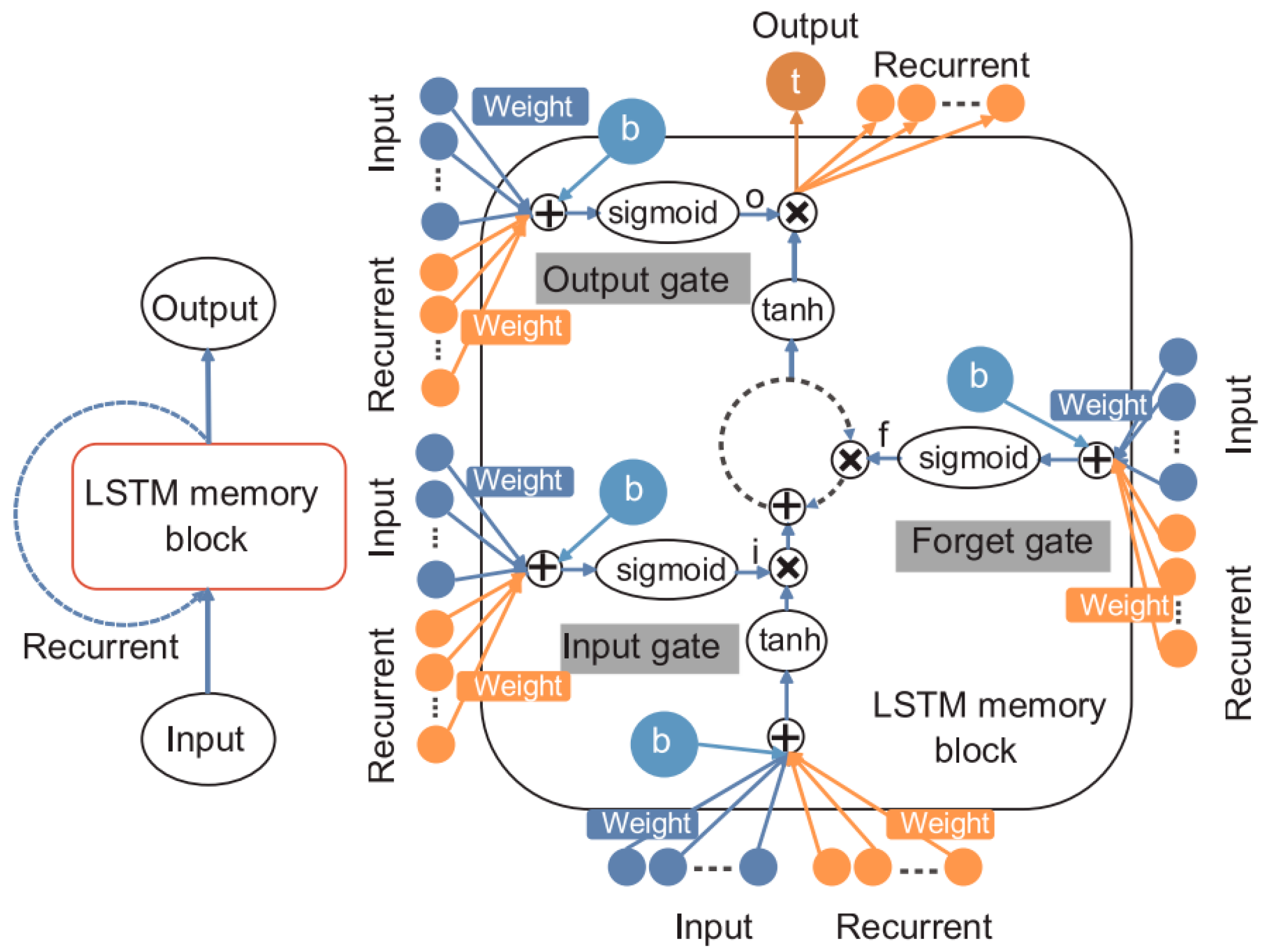
The LSTM model represents a type of recurrent neural network (RNN) in which the traditional hidden layer is replaced by a memory block that includes an input gate, an output gate, a memory cell, and a forget gate. The input gate is responsible for determining which new information should be stored in the memory cell state, while the forget gate determines which information should be removed from the cell state. The architecture of the LSTM model is depicted in Figure 2 [56].

Figure 2.
The design of the long short-term memory (LSTM) model adapted from [56].
The LSTM model’s overall memory block can be symbolized by Equations (5) and (6).
C denotes the state of the cell, with w and W representing the weights associated with the connections between gates and layers. Three biases are present: bi, bf, and bo. Activation functions are symbolized by σ and Tanh. Hochreiter and Schmidhuber offer a comprehensive explanation and utilization of LSTM [59,60].
In the realm of reservoir inflow prediction, LSTM models are employed to forecast upcoming inflow levels by analyzing historical data such as rainfall, temperature, and previous inflow quantities. The capacity of LSTM models to handle sequential data renders them especially valuable in detecting patterns and trends across time, essential for precise inflow forecasting. This capability can greatly benefit reservoir management by enhancing water storage optimization and flood prevention tactics.
2.4. Multiple Linear Regression (MLR)
Multiple linear regression (MLR) is a statistical method used to model the relationship between one dependent variable and two or more independent variables. MLR is complicated [44]. MLR, an error-based prediction model [61], predicts linearly from descriptive feature values. In weight space, gradient descent favors certain linear models. Equation (7) specifies the MLR model.
The vector of m defining features in d[m] has weights [m] equal to (m + 1). We can improve Equation (8) by adding a dummy defining feature, d[0], which is typically set to 1.
However, predictive analytics issues should not use random starting points. Gradient descent directs exploration from a random starting point. Using these approaches, randomly chosen weights must undergo minimum error gradient modifications to move on the error surface [62]. Performance increases with additional predictors in this optimization [44].
3. Research Methodology
3.1. Research Framework
The framework presented in Figure 3 outlines five key phases of the process as follows: The first phase involves data collection, where twelve variables, including monthly reservoir inflow and rainfall, were obtained from historical hydrological data. Additionally, eight sea surface temperature (SST) variables and two climatic indicators, the Southern Oscillation Index (SOI) and the Dipole Mode Index (DMI), were used to represent climate indices. In the second phase, the process is divided into two sub-stages. The first sub-stage focuses on integrating data from various sources into a cohesive dataset, while the second sub-stage transforms the data into lag features suitable for supervised learning. Reservoir inflow predictions for multi-step forecasting (T + 3, T + 6, T + 9, and T + 12) are based on the preceding time series values (T − 1 to T − 12). The data are then adjusted into a 12-month lag for the next phase. The third phase involves feature analysis and modeling, which consists of two sub-processes. First, feature selection (FS) is conducted to identify the optimal features. This process is based on our previous research [12]. In the second sub-process, quantile regression (QR) techniques with three different quantiles (75, 80, and 90) are applied to isolate extreme and normal events, determining the optimal threshold for data segmentation and preparing the data for further analysis in the subsequent phase.
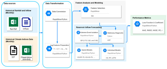
Figure 3.
The overview of the research framework.
3.2. Experimental Setup
Table 3 shows detailed information and a list of acronyms for the above-mentioned models. For the hybrid models, the first position refers to the model used for an extreme event, and the second one is a normal event, whereas both extreme and normal events were applied simultaneously to the individual machine learning models. Due to the limited data available at the 90th percentile (fewer than ten observations), twelve hybrid machine learning models based on two quartile thresholds (75 and 80) were used to assess performance. These hybrid models include XG-RF-75, XG-RF-80, RF-XG-75, RF-XG-80, RF-RF-75, RF-RF-80, XG-XG-75, XG-XG-80, MLR-XG-75, MLR-XG-80, XG-MLR-75, and XG-MLR-80. Additionally, four individual machine learning models (XG, RF, LSTM, and MLR) were also implemented. Notably, each individual model was applied to handle both extreme and normal events within the dataset. RF employs the bootstrap feature sampling principle for dimensions. Therefore, this approach is resistant to overfitting, thus negating the necessity for cross-validation [63]. Similarly, XGBoost utilizes a regularized model to prevent overfitting [53], a method previously employed in hydrological management analysis [58]. The input features for the ten hybrid and four individual models were optimally selected using a Genetic Algorithm (GA), as outlined in Section 3.1. Model performance was then assessed in the fourth stage through 10-fold cross-validation, employing evaluation metrics including MAE, RMSE, PE, NNSE, and the correlation coefficient (r). The investigation described in this case study employed a 64-bit computing system equipped with 16 GB of RAM to conduct various numerical experiments. Python 3.11 and RapidMiner Studio 9.9 were employed for the purpose of this analysis.
Table 3.
The experimental setup for the development of the reservoir inflow forecasting model under extreme events with climate indices.
3.3. Statistical Performance Measures
3.3.1. Mean Absolute Error (MAE)
The mean absolute error (MAE) demonstrates the average absolute deviation between the estimated values and the true value. The effectiveness of the model is indicated when the root mean square error (RMSE) and MAE values tend towards 0 [64], as illustrated in Equation (9).
where
= Observed or modeled data value at time step i;
= Predicted data value at time step i;
n = Total number of observations.
3.3.2. Root Mean Square Error (RMSE)
The root mean square error (RMSE) is commonly utilized as a standardized statistical metric for evaluating model performance in various fields, such as hydrology and meteorology. It is particularly applied to tasks including water level prediction, water inflow forecasting, air quality measurement, and climate research. The RMSE value serves as an indicator of the degree of inaccuracies present and is a statistical tool used to quantify the average error between expected and observed values. In the realm of model assessment, RMSE is most suitable for scenarios involving a Gaussian error distribution. Often, a combination of metrics, including RMSE and MAE, is needed for a comprehensive evaluation [64,65]. Equation (10) serves as a representation of RMSE.
where
= Observed or modeled data value at time step i;
= Predicted data value at time step i;
n = Total number of observations.
3.3.3. Centered Root Mean Square Error (CRMSE)
CRMSE measures the average magnitude of errors between predicted and observed values after removing any systematic bias [66]. In Taylor diagrams, CRMSE is represented as the radial distance between the model’s point and the reference point of the observed data. Equation (11) for the Centered Root Mean Square Error (CRMSE) is given by the following:
where
= Observed or modeled data value at time step i;
= Predicted data value at time step i;
= Mean of observed data values over the entire period;
= Mean of predicted data values over the entire period;
n = Total number of observations.
3.3.4. The Relative Peak Error (PE)
The relative peak error is a measure used primarily in the analysis of time series data, particularly in forecasting and modeling scenarios. It quantifies how accurately a model or method can predict the peak value of a dataset by comparing the predicted (or expected) peak value to the actual peak value observed [67]. The relative peak error is calculated with the following Equation (12):
The meanings of the three answers are as follows: PE = 0: The actual peak matches the expected peak perfectly. There is no error in the peak prediction. PE > 0: The actual peak exceeds the expected peak. This indicates an overestimation error where the model or method predicted less than the actual peak and PE < 0. The actual peak is less than the expected peak. This situation points to an underestimation error, where the model or method predicted more than the actual peak.
3.3.5. Normalized Nash–Sutcliffe Efficiency (NNSE)
Normalized Nash–Sutcliffe Efficiency (NNSE) is a modified version of the Nash–Sutcliffe Efficiency (NSE), as indicated by the following Equations (13) and (14), which are widely used metrics for evaluating the predictive accuracy of hydrological models. The NSE measures the relative magnitude of the residual variance compared to the observed data variance, providing an indication of how well the predicted values match the observed data [68].
where
= Predicted data value at time step i;
= Observed or modeled data value at time step i;
= Mean of observed data values over the entire period;
n = Total number of observations.
The NNSE normalizes this metric, providing a bound range for easier interpretation and comparison across different studies [69]. It is particularly useful in ensuring the performance metric is scaled between 0 and 1, making it more intuitive. An NNSE value closer to 1 indicates better model performance, while a value closer to 0 indicates poor model performance. To compute the NNSE, the NSE is transformed to fit within the desired normalized range. The exact normalization process can vary, but a common approach is to apply a linear transformation to the NSE values to ensure they fall within the [0, 1] range [58,68,69]. This normalization makes NNSE a convenient metric for comparing the efficiency of different models or different configurations of the same model.
3.3.6. Normalized Score
Each metric (i.e., MAE, RMSE, PE, and 1-NNSE) is normalized to a common scale (e.g., 0 to 1), where 0 represents the best possible score, and 1 represents the worst. These normalized metrics are then combined into an overall performance score.
3.3.7. Correlation Coefficient (r)
Pearson’s correlation coefficient is widely used in hydrology and other scientific research. It is calculated by dividing the covariance of two variables by the product of their standard deviations [44]. A covariance exceeding 0.7 suggests a notable relationship between anticipated and actual values [35,44]. This relationship can be mathematically represented by Equation (15).
where
= Observed or modeled data value at time step i;
= Predicted data value at time step i;
n = Total number of observations.
3.3.8. Augmented Dickey–Fuller Test (ADF)
The Augmented Dickey–Fuller (ADF) test is a widely used statistical test to determine whether a time series is stationary. Stationarity implies that the statistical properties of the time series, such as mean and variance, remain constant over time. The test is an augmented version of the Dickey–Fuller test, which was originally introduced by Dickey and Fuller (1979) to test for the presence of unit roots in time series data, a key indicator of non-stationarity [70].
The ADF test can be represented by the following regression Equation (16):
where is the first difference of the time series, t is the time trend, α is a constant (drift). β is the coefficient on the time trend, is the lagged value of the series, γ is the coefficient of the lagged level of the time series, which is crucial in testing for a unit root, are the coefficients of the lagged differences of the time series to account for higher-order autoregression. is the error term, assumed to be white noise.
The test statistic from the ADF test is compared against critical values from the Dickey–Fuller distribution. If the test statistic is less than the critical value, the null hypothesis of a unit root is rejected, implying that the series is stationary. Otherwise, if the test statistic is greater than the critical value, we fail to reject the null hypothesis, suggesting the series is non-stationary.
4. Results and Discussion
This section presents and analyzes two key findings and their implications: (1) the use of quartile regression to separate extreme and normal events, and (2) the performance comparison of 12 hybrid and 4 individual machine learning models across four forecast intervals—three, six, nine, and twelve months ahead. Details are provided in the following subsections.
4.1. Isolating Extreme and Normal Events Using Quantile Regression
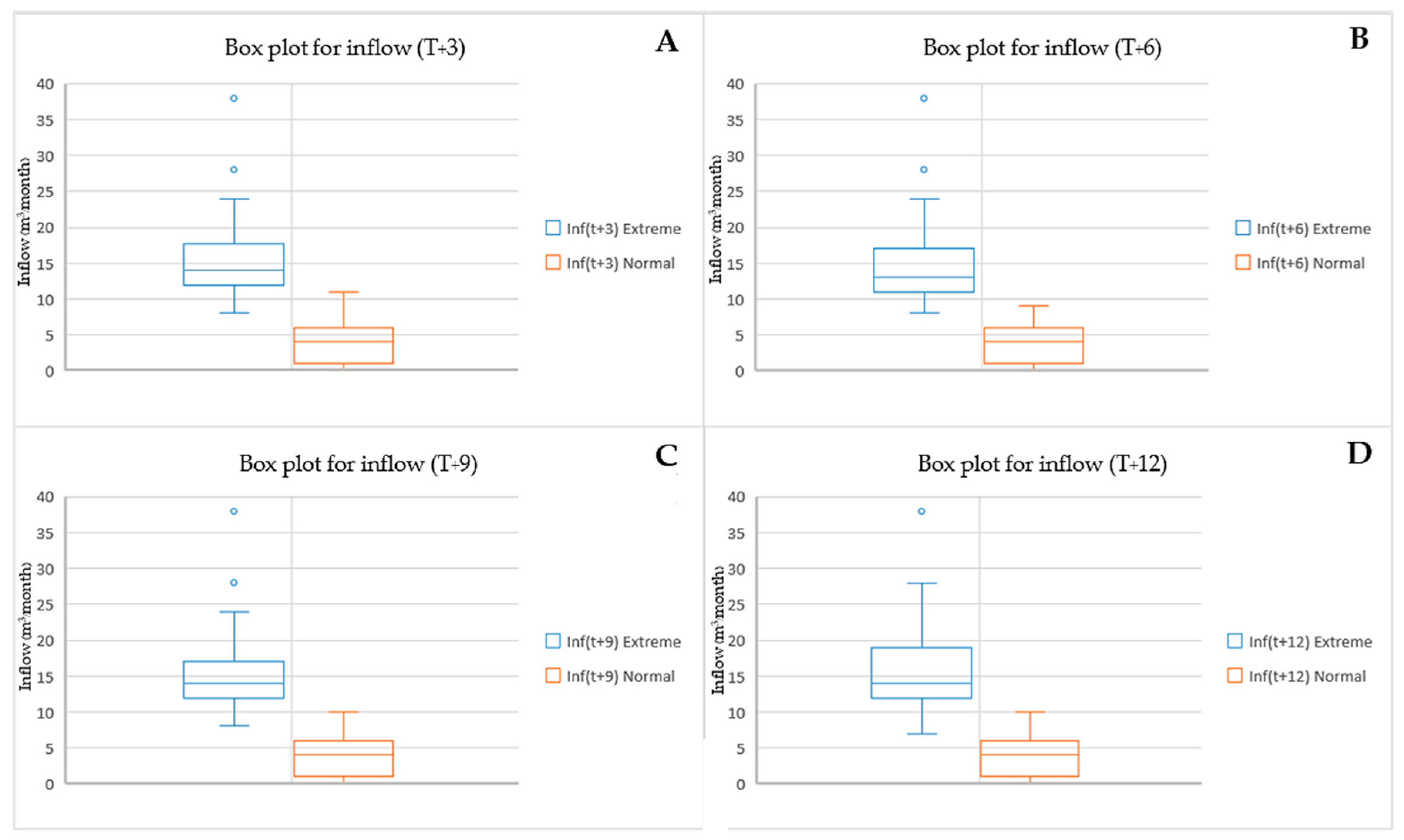
The findings of the study entail the examination of extreme occurrences through the utilization of the quantile methodology. The analyst applied quantile regression (QR) to distinguish data related to notable events. By conducting an experiment where quantile figures were segmented into three distinct trials, the objective was successfully accomplished. The data sets were separated by three quantile values of 0.75 (QR-75), 0.80 (QR-80), and 0.90 (QR-90) [40,70]. Figure 4, Figure 5 and Figure 6 present details on the essential statistical characteristics of each of the three datasets. The data for all four time periods is categorized based on lead time in the table. Extreme events and normal events are segregated into separate groups for each period, with each subset further divided into data sets. The box and whisker diagrams illustrate baseline statistics for extreme and normal event data at four lead times using QR-75, QR-80, and QR-90. Figure 4 presents detailed statistics on reservoir inflow for each lead time, including the total amount, average, standard deviation, minimum, and maximum values. The specifics are as follows:
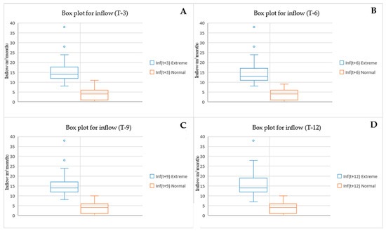
Figure 4.
Box plot (QR-75) for extreme and normal event data across four lead times.
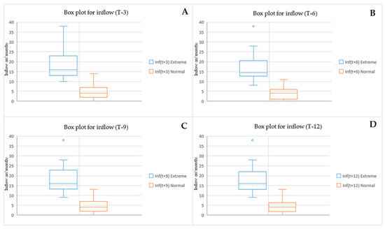
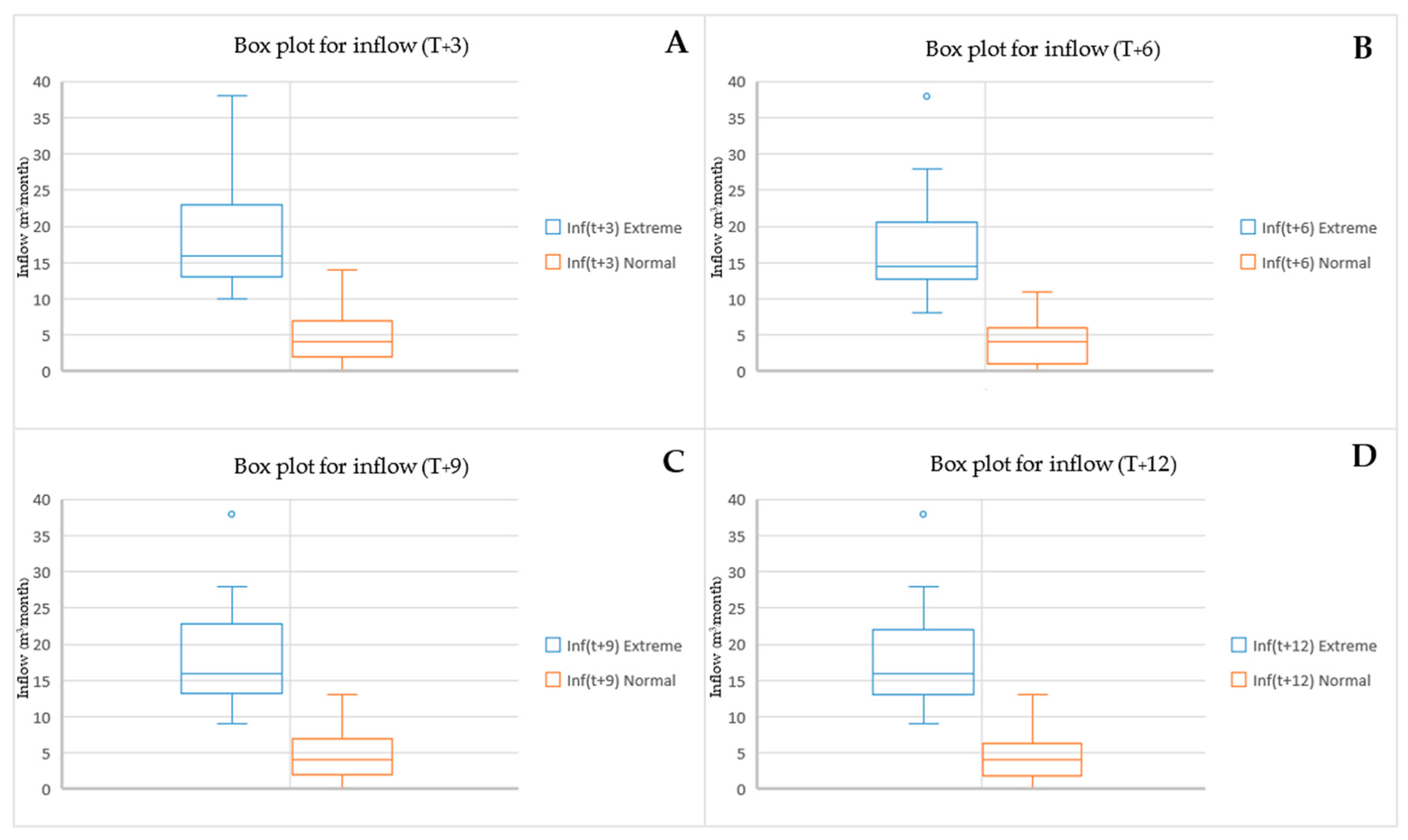
Figure 5.
Box plot (QR-80) for extreme and normal event data across four lead times.
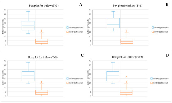
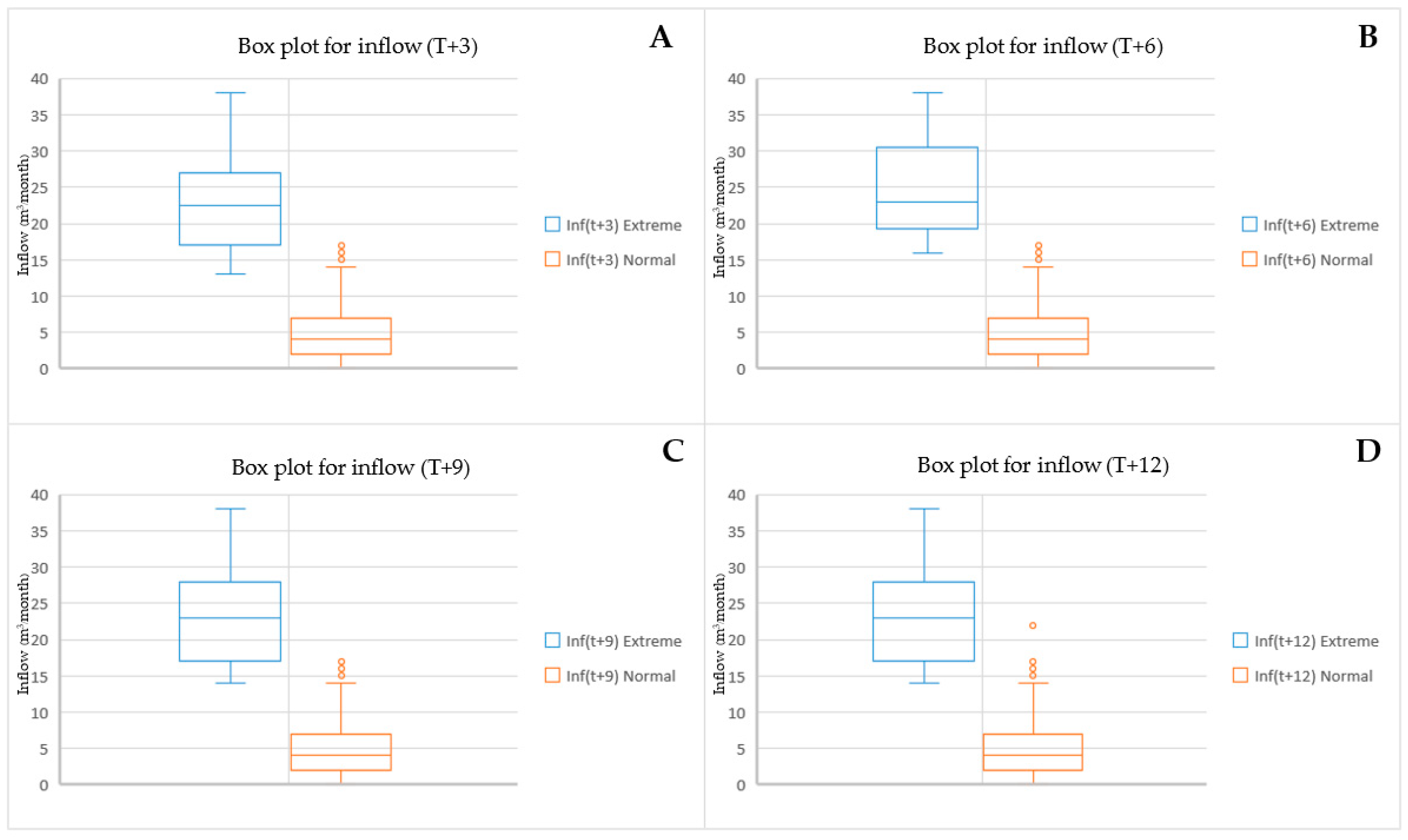
Figure 6.
Box plot (QR-90) for extreme and normal event data across four lead times.
For a QR of 0.75 at lead time T + 3 (see Figure 4A), the extreme events’ statistical characteristics of the dataset are 34, 15.64, 6.11, 8, and 38, respectively. The statistics for the normal datasets are 160, 3.80, 2.72, 0, and 11, respectively. At T + 6 (see Figure 4B), the extreme events’ statistical characteristics of the dataset are 37, 15.81, 7.19, 8, and 38, respectively. The statistics for the normal datasets are 156, 3.66, 2.63, 0, and 9, respectively. At T + 9 (see Figure 4C), the extreme events’ statistical characteristics of the dataset are 35, 16.12, 7.24, 8, and 38, respectively. The statistics for the normal datasets are 158, 3.76, 2.70, 0, and 10, respectively. At the last lead time (T + 12), as shown in Figure 4D, the extreme events’ statistical characteristics of the dataset are 35, 15.88, 6.99, 7, and 38, respectively. The statistics for the normal datasets are 158, 3.83, 2.79, 0, and 10, respectively.
For a QR of 0.80 at lead time T + 3 (see Figure 5A), the extreme events’ statistical characteristics of the dataset are 23, 18.48, 7.63, 10, and 38, respectively. The statistics for the normal datasets are 170, 4.26, 3.27, 0, and 14, respectively. At T + 6 (see Figure 5B), the extreme events’ statistical characteristics of the dataset are 30, 17.13, 7.16, 8, and 38, respectively. The statistics for the normal datasets are 163, 3.9, 2.82, 0, and 11, respectively. At T + 9 (see Figure 5C), the extreme events’ statistical characteristics of the dataset are 24, 18.33, 7.51, 9, and 38, respectively. The statistics for the normal datasets are 169, 4.24, 3.19, 0, and 13, respectively. At the last lead time (T + 12), as shown in Figure 5D, the extreme events’ statistical characteristics of the dataset are 27, 18, 7.19, 9, and 38, respectively. The statistics for the normal datasets are 166, 4.14, 3.08, 0, and 13, respectively.
For a QR of 0.90 at lead time T + 3 (see Figure 6A), the extreme events’ statistical characteristics of the dataset are 12, 23.08, 7.85, 13, and 38, respectively. The statistics for the normal datasets are 181, 4.82, 3.9, 0, and 17, respectively. At T + 6 (see Figure 6B), the extreme events’ statistical characteristics of the dataset are 10, 24.9, 7.31, 16, and 38, respectively. The statistics for the normal datasets are 183, 4.92, 4.01, 0, and 17, respectively. At T + 9 (see Figure 6C), the extreme events’ statistical characteristics of the dataset are 11, 24, 7.56, 14, and 38, respectively. The statistics for the normal datasets are 182, 4.91, 3.95, 0, and 17, respectively. At the last lead time (T + 12), as shown in Figure 6D, the extreme events’ statistical characteristics of the dataset are 11, 23.64, 7.76, 14, and 38, respectively. The statistics for the normal datasets are 182, 5.02, 4.17, 0, and 22, respectively.
The statistical analysis across the three quantile scenarios aligns with recommendations by Austin et al. (2015) [71] and Schmidt & Finan (2018) [72], which suggest a minimum of ten observations for reliable regression analysis. Additionally, the ADF test yielded a result of -3.554 with a p-value of 0.0067 (p < 0.05), rejecting the null hypothesis of non-stationarity and indicating that the dataset is likely stationary. Previous studies have isolated extreme events from entire datasets using methods such as wavelet transform and quantile regression [69,73,74,75,76]. The wavelet transform, however, is particularly suited for non-stationary data [74,75]. Typically, quantile regression (QR) is applied in regression forecasting rather than for isolating extreme events. In this study, the research team utilized QR to partition the data, as QR effectively distinguishes extreme events by considering quantiles in both input and output variables. This approach aligns with Hauswirth et al. (2023) [77], who separated data by the highest and lowest 30% of records, using the highest quantile data to forecast flood events.
4.2. Developing Reservoir Inflow Forecasting Models Under Extreme Events
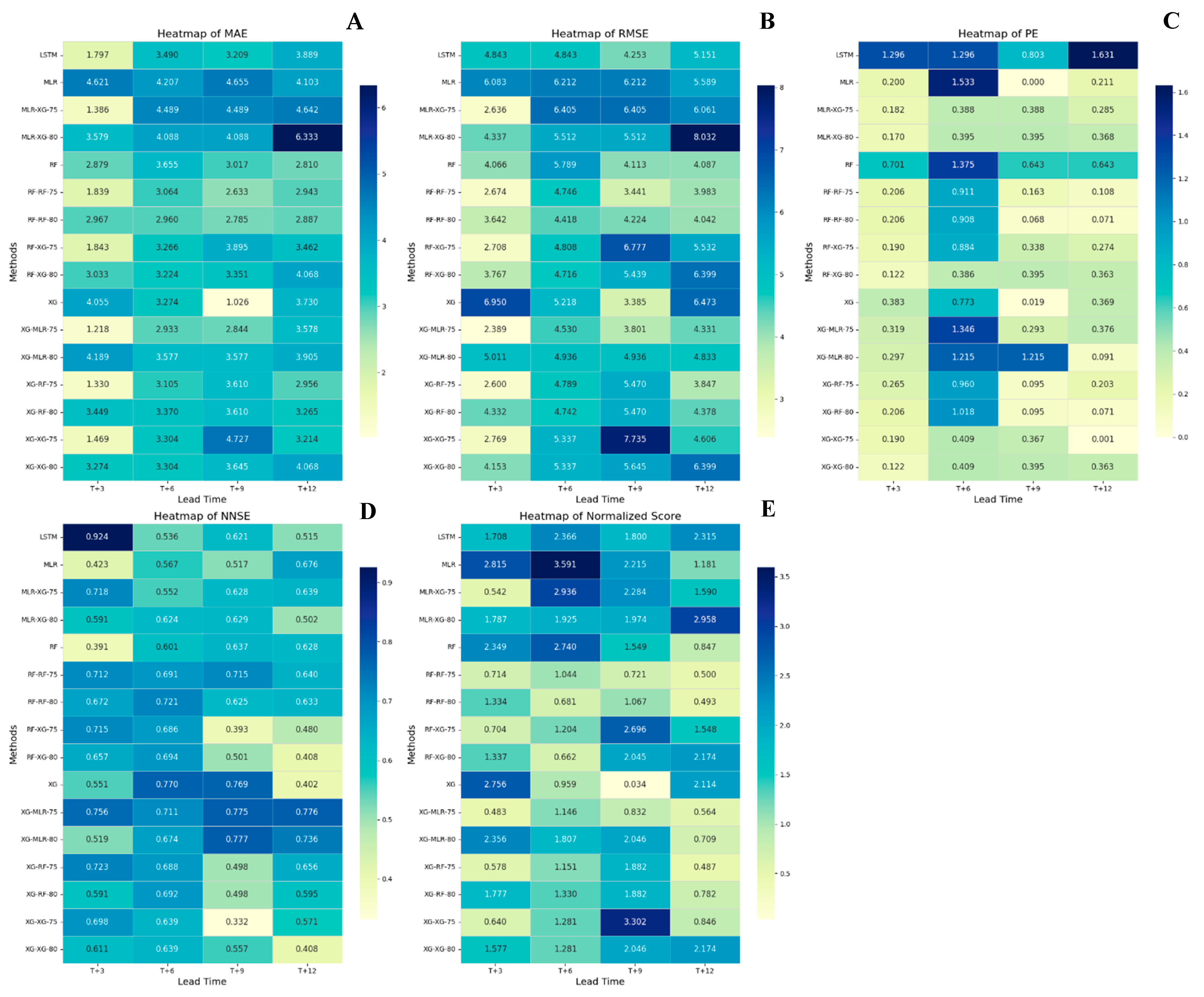
Figure 7 presents a heat map displaying the statistical performance metrics (MAE, RMSE, PE, NNSE, and normalized score) for all 16 ML techniques, organized by forecast lead times: T + 3, T + 6, T + 9, and T + 12. The key result observations are as follows.

Figure 7.
A heatmap displaying the statistical performance metrics (MAE, RMSE, PE, NNSE, and normalized score) for all 16 ML techniques, organized by forecast lead times: T + 3, T + 6, T + 9, and T + 12.
At lead time T + 3, the XG-MLR-75 model has the lowest normalized score (0.483), suggesting it performs the best among all models, particularly for MAE, RMSE, and NNSE. LSTM achieves the highest NNSE (0.924), indicating excellent predictive power, but has a relatively high normalized score (1.708) due to high errors in other metrics. MLR has the highest normalized score (2.815), indicating lower performance compared to other models.
At lead time T + 6, the RF-XG-80 model has the lowest normalized score (0.662), indicating it has the best performance among all models at T + 6, with balanced performance across MAE, RMSE, and NNSE. The RF-RF-80 (0.681) and XG-75 (0.959) are close competitors, performing well on key metrics but with slightly higher MAE or RMSE than the RF-XG-80. LSTM-75 has a relatively high normalized score (2.366) due to a high 1-NNSE and PE, indicating it may not generalize as well for this lead time. The MLR-GA-75 model has the highest normalized score (3.591), primarily due to high MAE, RMSE, and PE, suggesting it is less effective for this T + 6 forecast.
At lead time T + 9, the XG-75 model has the lowest normalized score (0.034), suggesting it has the best overall performance among the models tested. It also has the lowest MAE (1.026), RMSE (3.385), and PE (0.019), indicating it is a strong model for this forecasting task. The RF-RF-75 and XG-MLR-75 also perform reasonably well, with normalized scores of 0.721 and 0.832, respectively. However, they have higher MAE and RMSE values compared to XG-75, showing that they are less accurate but still competitive. At the same time, the XG-XG-75 has the highest normalized score (3.302), indicating poor performance. It also has high error metrics (MAE = 4.727, RMSE = 7.735) and is the least efficient according to NNSE (0.332).
At lead time T + 12, the XG-RF-75 has a normalized score of 0.487, with relatively low MAE (2.955) and RMSE (3.847). It performs well across several error metrics, indicating it is a strong model for the given forecast. The RF-RF-80 is another strong performer with a normalized score of 0.493, showing good accuracy with an MAE of 2.887 and an RMSE of 4.042. At the same time, the MLR-XG-80 has the highest normalized score of 2.958, which indicates the poorest performance. This model also has the highest MAE (6.333) and RMSE (8.032), suggesting it struggles with making accurate predictions for this lead time. Additionally, the XG-75 and XG-XG-80 also show relatively high normalized scores (2.114 and 2.174, respectively), indicating weaker performance when compared to models like the XG-RF-75 or RF-RF-80.
In summary, the results show that combining quantile regression (QR) to distinguish between extreme and normal events with hybrid models significantly improves the accuracy of monthly reservoir inflow forecasting, except for the 9-month lead time, where the XG model continues to deliver the best performance. The top-performing models, based on normalized scores for 3-, 6-, 9-, and 12-month-ahead forecasts, are XG-MLR-75, RF-XG-80, XG-75, and XG-RF-75, respectively. For method comparisons, tree-base methods, particularly those involving combinations of XGBoost and RF, demonstrate superior performance across multiple metrics. This aligns with the established understanding that tree-base methods can leverage the strengths of individual models to enhance overall predictive accuracy [44,45]. The consistent performance of RF-XG-75 across metrics suggests it is particularly well-suited for the given predictive task.
This study aligns with and extends the findings of several previous works in hydrological forecasting and climate impact studies. The superior performance of hybrid models, particularly those combining RF and XGBoost, is in line with the results obtained by Yin et al. [70], who found that ensemble methods significantly reduced prediction errors and improved model robustness in hydrological forecasting. XGBoost is a powerful ensemble learning algorithm based on gradient boosting, well-known for handling non-linear relationships effectively due to its ability to create successive decision trees that correct errors from previous iterations. However, XGBoost can be prone to overfitting, especially when dealing with imbalanced datasets or extreme events. Zheng et al. (2022) [35] support this limitation by finding that XGBoost tends to overemphasize small variations in the data. On the other hand, Yin et al. (2017) [70] showed that hybrid models combining it with other techniques like RF significantly improve performance in extreme conditions due to reduced overfitting. As shown in earlier research (e.g., Wei et al., 2020 and Wei et al., 2022 [78,79]), similar to the research report by Ibrahim et. al., it was found that the ensemble technique (XGboost) overall outperformed other techniques (ANN, SVR, and ANFIS) for multi-step monthly reservoir inflow forecasting [55]. Particularly when the model is integrated with FS, the integration of GA for FS is supported by similar findings from Alquraishi et al. and Yang et al. [34,53]. Using data on climate indices, especially the SOI, DMI, and SST, is similar to what Amnatsan et al. and Kim et al. [12,37] did, and it works very well for making predictions.
Considering model performance across four lead times, it was found that lead time T + 3 (XG-MLR-75) provides a good balance of MAE, RMSE, NNSE, and a relatively low normalized score of 0.483, making it a solid choice for short-term forecasting. Lead time T + 6 (RF-XG-80) has the highest MAE and RMSE values, indicating poorer performance. Its normalized score of 0.662 is also higher, reflecting less efficiency in its predictions. Lead time T + 9 (XG-75) performs the best overall, with the lowest MAE, RMSE, and normalized score of 0.034. This indicates excellent prediction performance and a good fit to the observed data. And lead time T + 12 (XG-RF-75) shows performance similar to XG-MLR-75 but slightly worse in most metrics, with a normalized score of 0.487. XG-75 (T + 9) is the top-performing model based on the normalized score, indicating it provides the best balance between accuracy and fitting the observed data. XG-MLR-75 (T + 3) is a good option for shorter lead times but is outperformed by XG-75 for longer-term forecasts. XG-RF-75 (T + 12) shows moderate performance across most metrics, with higher MAE and RMSE compared to the top-performing models, indicating a less accurate fit to the observed data for longer-term forecasts. RF-XG-80 (T + 6) performs poorly across most metrics, especially with higher MAE and RMSE. These results are consistent with previous studies that show a decline in prediction accuracy as lead time increases [72,78,79]. The main factors contributing to this are as follows: model characteristics and error propagation. The complexity of the model and the accumulation of errors over time have varying impacts on performance at different lead times. Additionally, temporal variability and data dynamics, including fluctuations and errors in the data over time, can lead to variations in accuracy at different forecast intervals. Finally, error distribution and seasonal effects play a significant role, as models respond to seasonal and cyclical patterns differently depending on the forecast horizon.
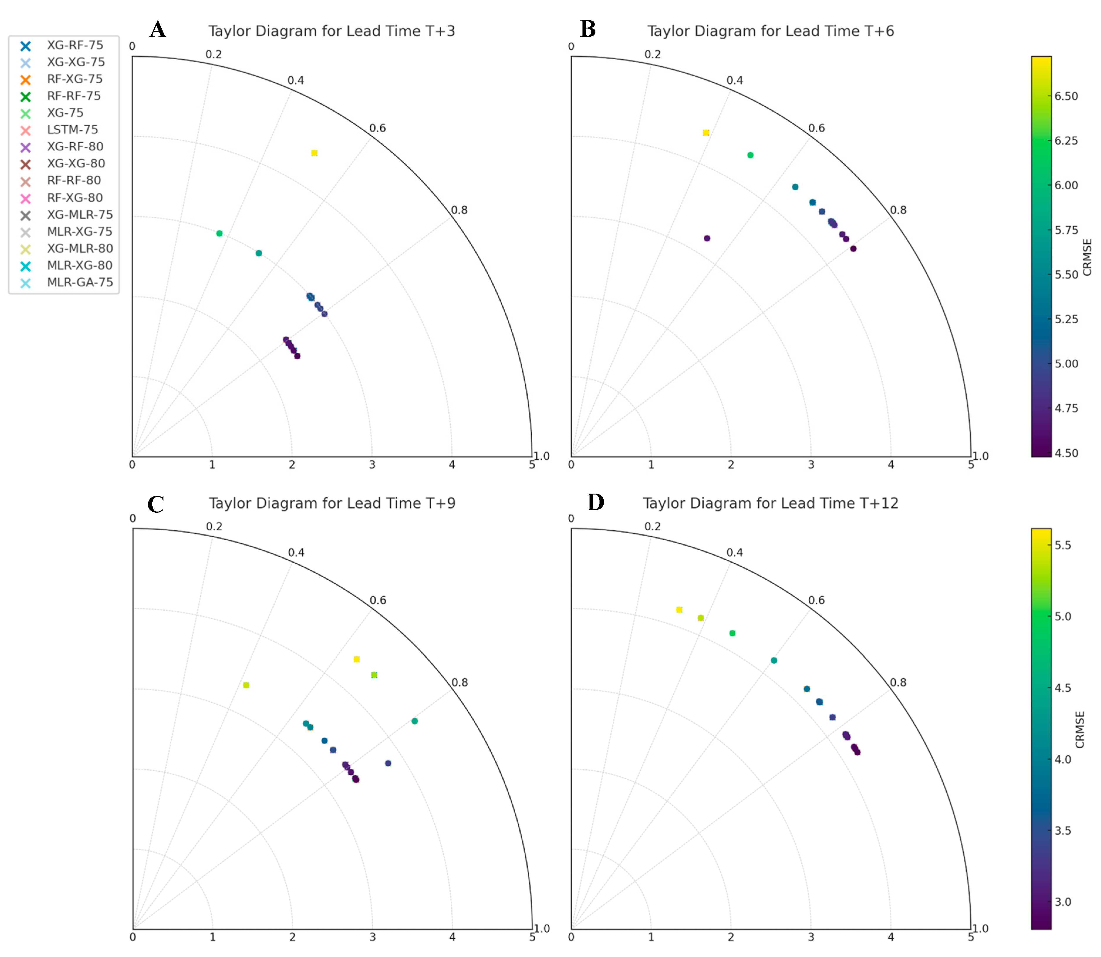
This analysis uses Taylor diagrams to compare model performance across four different lead times: 3, 6, 9, and 12 (see Figure 8A–D). The Taylor diagram succinctly displays three key metrics: the correlation coefficient (r), the standard deviation (SD), and the centered root mean square error (CRMSE) is the difference between the simulated and observed patterns is proportional to the distance to the point on the x-axis labeled “observed” [70] CRMSE has a lead time of T + 3, ranging from 2.388 to 6.695. The “XG-MLR-75” model has the lowest CRMSE, indicating the most accurate forecasts with the least error. Model correlations range from 0.364 to 0.854. The “XG-MLR-75” model has the highest correlation coefficient, showing a linear relationship between predicted and observed values. The “XG-75” model has the largest standard deviation, indicating greater forecast variability.
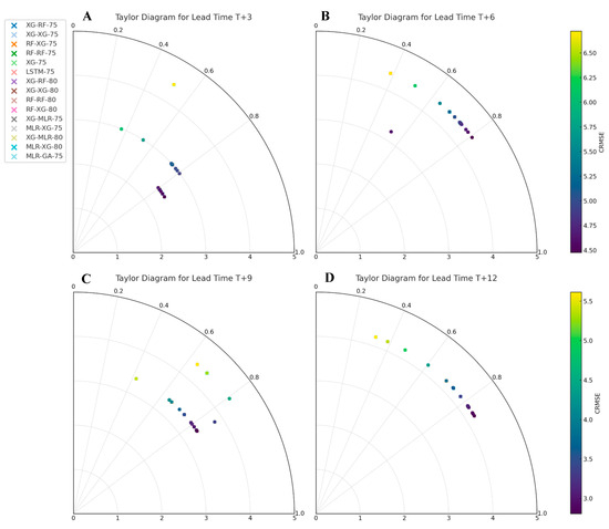
Figure 8.
The Tylor diagram for four lead times.
CRMSE ranges from 4.42 to 6.405 for a T + 6 lead time. Low CRMSE means that the “RF-RF-80” model makes the most accurate predictions with the least error. Model correlations range from 0.384 to 0.805. The “XG-MLR-80” model has the highest correlation coefficient, showing a linear relationship between predicted and observed values. Most models had standard deviations of 7.105, indicating similar prediction variability.
The CRMSE values for lead time T + 9 range from 3.385 to 7.735. The “XG-75” model has the lowest CRMSE, indicating the most accurate forecasts with the least error. Model correlations range from 0.422 to 0.839. The “XG-75” model has the highest correlation coefficient, showing a linear relationship between predicted and observed values. Standard deviations are 5.449–7.105. The “MLR-XG-75” model has the largest standard deviation, indicating the most forecast variability.
For lead time T + 12, CRMSE ranges from 3.805 to 8.032. Low CRMSE means the “XG-RF-75” model makes the most accurate predictions with the least error. Model correlations range from 0.321 to 0.851. The “RF-RF-80” model has the highest correlation coefficient, showing a linear relationship between predicted and observed values. Most models have standard deviations of 5.311, showing comparable forecast variability.
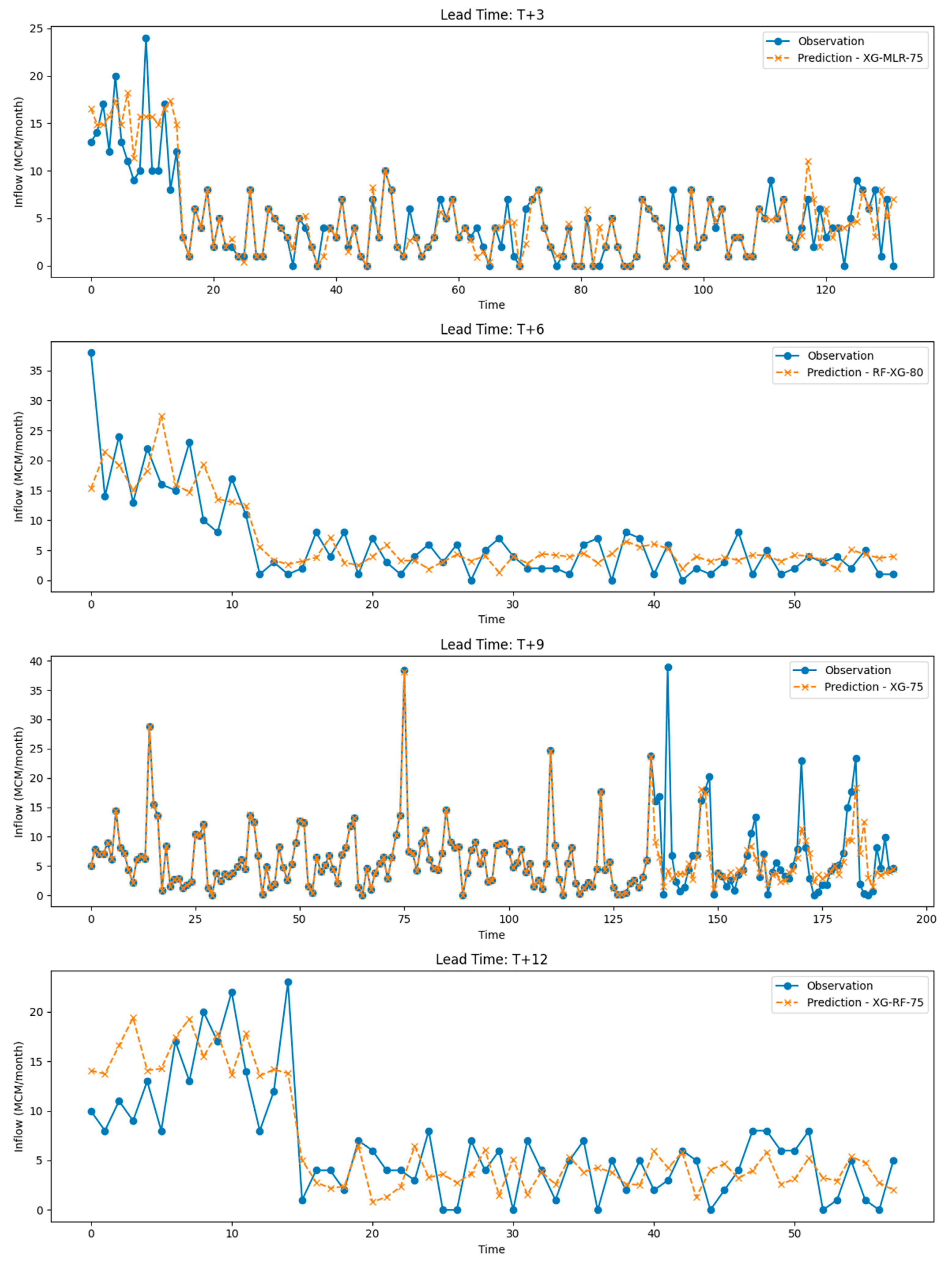
Figure 9 presents a comparison between observed and predicted reservoir inflows from the top-performing models across four lead times (T + 3, T + 6, T + 9, and T + 12).
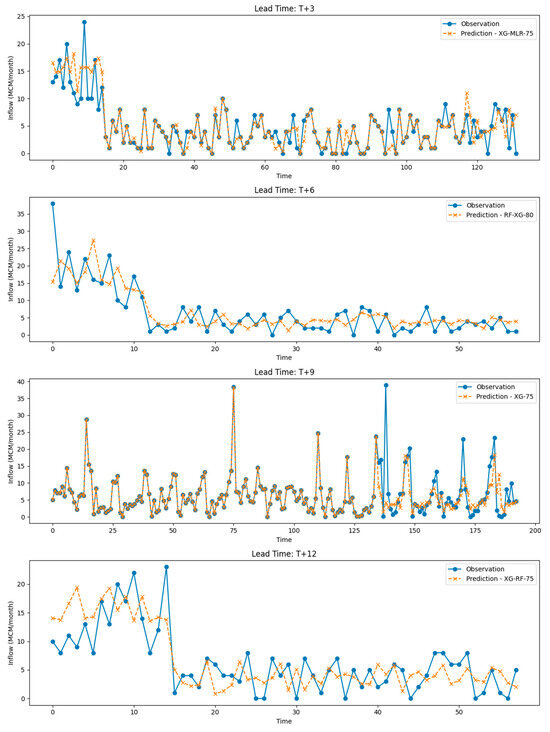
Figure 9.
A comparison between observed and predicted reservoir inflows from the top-performing models across four lead times (T + 3, T + 6, T + 9, and T + 12).
4.3. Future Works
Future research could focus on enhancing tree-based machine learning methods by integrating additional machine learning techniques or optimizing the parameters of existing methods to further improve predictive accuracy and performance. Developing models tailored to specific lead times could enhance prediction accuracy. For example, short-term models may benefit from distinct features or techniques compared to medium-term models. Experimenting with additional input variables, particularly climate indicators that influence Thailand’s climate conditions, along with the application of advanced feature engineering methods, could further reduce prediction errors and improve model performance.
5. Conclusions
This study presents a novel approach to enhancing reservoir inflow forecasting accuracy, which is crucial for effective water resource planning and management. The research utilizes quantile regression (QR) in combination with various machine learning techniques, including tree-based methods (Random Forest and XGBoost), traditional regression (Multiple Linear Regression), and neural networks (LSTM), to forecast reservoir inflows across four different lead times using 18 years of monthly data from the Huai Nam Sai reservoir in southern Thailand. The key research findings could be concluded as follows:
- Using quantile regression (QR) to isolate extreme and normal events significantly improved reservoir inflow forecasting performance compared to developing a machine learning model with the entire dataset, except for the T + 9 lead time. Additionally, the study found that using QR-75 to isolate the dataset outperformed QR-80 in three of the four lead times.
- Among the four lead times, hybrid models demonstrated improved forecasting performance, with XG-MLR-75 performing best at T + 3, RF-XG-80 at T + 6, and XG-RF-75 at T + 12. However, at the T + 6 lead time, XG outperformed all other 15 machine learning models
- Another important finding of this research is the uneven decline in prediction accuracy as lead time increases. Specifically, the model performed best at T + 9, followed by T + 3, T + 12, and T + 6 in that order. This pattern is influenced by factors such as model characteristics, error propagation, temporal variability, data dynamics, and seasonal effects.
Author Contributions
Conceptualization, P.D. and N.K.; methodology, J.W., P.D. and N.K.; software, J.W.; validation, P.D. and N.K.; formal analysis, J.W.; investigation, J.W., P.D. and N.K.; resources, J.W. and N.K.; data curation, J.W.; writing—original draft preparation, J.W., P.D. and N.K.; writing—review and editing, P.D., N.K. and Q.B.P.; visualization, J.W.; supervision, P.D., N.K. and Q.B.P.; project administration, P.D. and N.K.; funding acquisition, J.W. and Q.B.P. All authors have read and agreed to the published version of the manuscript.
Funding
This research was partially funded by the Ministry of Higher Education, Science, Research, and Innovation, Thailand under grant number 6/2565. The authors are gratefully acknowledged.
Data Availability Statement
The datasets presented in this article are not readily available because the data are part of an ongoing study.
Conflicts of Interest
The authors declare no conflicts of interest.
References
- IPCC. Climate Change 2021: The Physical Science Basis. Intergovernmental Panel on Climate Change. 2021. Available online: www.ipcc.ch (accessed on 18 April 2024).
- Jha, M.K. Natural and anthropogenic disasters: An overview. In Natural and Anthropogenic Disasters: Vulnerability, Preparedness and Mitigation; Springer: Berlin/Heidelberg, Germany, 2010; pp. 1–16. [Google Scholar] [CrossRef]
- Ding, D.; Zhang, M.; Pan, X.; Yang, M.; He, X. Modeling extreme events in time series prediction. In Proceedings of the 25th ACM SIGKDD International Conference on Knowledge Discovery & Data Mining, Anchorage, AK, USA, 4–8 August 2019; Volume 1, pp. 1114–1122. [Google Scholar] [CrossRef]
- Kennedy, A.C.; Lindsey, R. What s the Difference Between Global Warming and Climate Change? ClimateWatch Magazine. 2015. Available online: https://climate.nasa.gov/faq/12/whats-the-difference-between-climate-change-and-global-warming/ (accessed on 25 October 2019).
- Vicente-Serrano, S.M.; Zabalza-Martínez, J.; Borràs, G.; López-Moreno, J.; Pla, E.; Pascual, D.; Savé, R.; Biel, C.; Funes, I.; Azorin-Molina, C.; et al. Extreme hydrological events and the influence of reservoirs in a highly regulated river basin of northeastern Spain. J. Hydrol. Reg. Stud. 2017, 12, 13–32. [Google Scholar] [CrossRef]
- Yu, Y.; Wang, P.; Wang, C.; Qian, J.; Hou, J. Combined Monthly Inflow Forecasting and Multiobjective Ecological Reservoir Operations Model: Case Study of the Three Gorges Reservoir. J. Water Resour. Plan. Manag. 2017, 143, 05017004. [Google Scholar] [CrossRef]
- Trenberth, K.E.; Dai, A.; Rasmussen, R.M.; Parsons, D.B. The changing character of precipitation. Bull. Am. Meteorol. Soc. 2003, 84, 1205–1217+1161. [Google Scholar] [CrossRef]
- Van Loon, A.F.; Van Lanen, H.A.J. Making the distinction between water scarcity and drought using an observation-modeling framework. Water Resour. Res. 2013, 49, 1483–1502. [Google Scholar] [CrossRef]
- Wheater, H.S. Water in a Changing World. 2000. Available online: https://www.worldscientific.com/doi/abs/10.1142/9781848160682_0002 (accessed on 17 February 2024).
- Office of the National Economic and Social Development Board. The Twelfth National Economic and Social. Office of the National Economic and Social Development Board Office of the Prime Minister Bangkok, Thailand. pp. 1–30. 2017. Available online: https://www.nesdc.go.th/ewt_dl_link.php?nid=9640 (accessed on 10 October 2024).
- Tongsiri, J.; Kangrang, A. Prediction of Future Inflow under Hydrological Variation Characteristics and Improvement of Nam Oon Reservoir Rule Curve using Genetic Algorithms Technique. Mahasarakham Univ. J. Sci. Technol. 2018, 37, 775–788. [Google Scholar]
- Kim, T.; Shin, J.Y.; Kim, H.; Kim, S.; Heo, J.H. The use of large-scale climate indices in monthly reservoir inflow forecasting and its application on time series and artificial intelligence models. Water 2019, 11, 374. [Google Scholar] [CrossRef]
- Othman, F.; Naseri, M. Reservoir inflow forecasting using artificial neural network. Int. J. Phys. Sci. 2011, 6, 434–440. [Google Scholar]
- Razavi, S.; Araghinejad, S. Reservoir inflow modeling using temporal neural networks with forgetting factor approach. Water Resour. Manag. 2009, 23, 39–55. [Google Scholar] [CrossRef]
- Chibanga, R.; Berlamont, J.; Vandewalle, J. Modelling and forecasting of hydrological variables using artificial neural networks: The Kafue River sub-basin. Hydrol. Sci. J. 2003, 48, 363–379. [Google Scholar] [CrossRef]
- Chiamsathit, C.; Adeloye, A.J.; Bankaru-Swamy, S. Inflow forecasting using artificial neural networks for reservoir operation. Proc. Int. Assoc. Hydrol. Sci. 2016, 373, 209–214. [Google Scholar] [CrossRef]
- Li, B.; Yang, G.; Wan, R.; Dai, X.; Zhang, Y. Comparison of random forests and other statistical methods for the prediction of lake water level: A case study of the Poyang Lake in China. Hydrol. Res. 2016, 47, 69–83. [Google Scholar] [CrossRef]
- Ivanciuc, O. Applications of Support Vector Machines in Chemistry. Rev. Comput. Chem. 2007, 23, 291–400. [Google Scholar] [CrossRef]
- Loucks, D.P.; van Bee, E. Water Resource Systems Planning and Analysis; Springer: Berlin/Heidelberg, Germany, 2017. [Google Scholar] [CrossRef]
- Mishra, A.K.; Singh, V.P. A review of drought concepts. J. Hydrol. 2010, 391, 202–216. [Google Scholar] [CrossRef]
- Vadiati, M.; Yami, Z.R.; Eskandari, E.; Nakhaei, M.; Kisi, O. Application of artificial intelligence models for prediction of groundwater level fluctuations: Case study (Tehran-Karaj alluvial aquifer). Environ. Monit. Assess. 2022, 194, 619. [Google Scholar] [CrossRef] [PubMed]
- Samani, S.; Vadiati, M.; Azizi, F.; Zamani, E.; Kisi, O. Groundwater Level Simulation Using Soft Computing Methods with Emphasis on Major Meteorological Components. Water Resour. Manag. 2022, 36, 3627–3647. [Google Scholar] [CrossRef]
- Ditthakit, P.; Pinthong, S.; Salaeh, N.; Binnui, F.; Khwanchum, L.; Pham, Q.B. Using machine learning methods for supporting GR2M model in runoff estimation in an ungauged basin. Sci. Rep. 2021, 11, 19955. [Google Scholar] [CrossRef]
- Lin, G.F.; Chen, G.R.; Huang, P.Y. Effective typhoon characteristics and their effects on hourly reservoir inflow forecasting. Adv. Water Resour. 2010, 33, 887–898. [Google Scholar] [CrossRef]
- Lee, D.; Kim, H.; Jung, I.; Yoon, J. Monthly reservoir inflow forecasting for dry period using teleconnection indices: A statistical ensemble approach. Appl. Sci. 2020, 10, 3470. [Google Scholar] [CrossRef]
- Weekaew, J.; Ditthakit, P.; Kittiphattanabawon, N. Reservoir Inflow Time Series Forecasting Using Regression Model with Climate Indices. Recent Adv. Inf. Commun. Technol. 2021, 251, 127–136. [Google Scholar]
- Alquraish, M.M.; Abuhasel, K.A.; Alqahtani, A.S.; Khadr, M. A comparative analysis of hidden markov model, hybrid support vector machines, and hybrid artificial neural fuzzy inference system in reservoir inflow forecasting (Case study: The king fahd dam, saudi arabia). Water 2021, 13, 1236. [Google Scholar] [CrossRef]
- Makridakis, S. Time series prediction: Forecasting the future and understanding the past. Int. J. Forecast. 1994, 10, 463–466. [Google Scholar] [CrossRef]
- Cheng, C.-T.; Feng, Z.-K.; Niu, W.-J.; Liao, S.-L. Heuristic Methods for Reservoir Monthly Inflow Forecasting: A Case Study of Xinfengjiang Reservoir in Pearl River, China. Water 2015, 7, 4477–4495. [Google Scholar] [CrossRef]
- Bai, Y.; Chen, Z.; Xie, J.; Li, C. Daily reservoir inflow forecasting using multiscale deep feature learning with hybrid models. J. Hydrol. 2016, 532, 193–206. [Google Scholar] [CrossRef]
- Weekaew, J.; Ditthakit, P.; Pham, Q.B.; Kittiphattanabawon, N.; Linh, N.T.T. Comparative Study of Coupling Models of Feature Selection Methods and Machine Learning Techniques for Predicting Monthly Reservoir Inflow. Water 2022, 14, 4029. [Google Scholar] [CrossRef]
- Luo, X.; Liu, P.; Dong, Q.; Zhang, Y.; Xie, K.; Han, D. Exploring the role of the long short-term memory model in improving multi-step ahead reservoir inflow forecasting. J. Flood Risk Manag. 2022, 16, e12854. [Google Scholar] [CrossRef]
- Liao, S.; Liu, Z.; Liu, B.; Cheng, C.; Jin, X.; Zhao, Z. Multistep-ahead daily inflow forecasting using the ERA-Interim reanalysis data set based on gradient-boosting regression trees. Hydrol. Earth Syst. Sci. 2020, 24, 2343–2363. [Google Scholar] [CrossRef]
- Tabari, H. Extreme value analysis dilemma for climate change impact assessment on global flood and extreme precipitation. J. Hydrol. 2021, 593, 125932. [Google Scholar] [CrossRef]
- Zhang, W.; Wang, H.; Lin, Y.; Jin, J.; Liu, W.; An, X. Reservoir inflow predicting model based on machine learning algorithm via multi-model fusion: A case study of Jinshuitan river basin. IET Cyber-Systems Robot. 2021, 3, 265–277. [Google Scholar] [CrossRef]
- Yang, S.C.; Yang, T.H. Uncertainty Assessment: Reservoir Inflow Forecasting with Ensemble Precipitation Forecasts and HEC-HMS. Adv. Meteorol. 2014, 2014, 1–11. [Google Scholar] [CrossRef]
- Amnatsan, S.; Yoshikawa, S.; Kanae, S. Improved forecasting of extreme monthly reservoir inflow using an analogue-based forecasting method: A case study of the Sirikit Dam in Thailand. Water 2018, 10, 1614. [Google Scholar] [CrossRef]
- Huang, I.H.; Chang, M.J.; Lin, G.F. An optimal integration of multiple machine learning techniques to real-time reservoir inflow forecasting. Stoch. Environ. Res. Risk Assess. 2022, 36, 1541–1561. [Google Scholar] [CrossRef]
- Chen, X.; Gupta, L.; Tragoudas, S. Improving the Forecasting and Classification of Extreme Events in Imbalanced Time Series Through Block Resampling in the Joint Predictor-Forecast Space. IEEE Access 2022, 10, 121048–121079. [Google Scholar] [CrossRef]
- Koenker, R.; Bassett, G. Regression Quantiles. Econometrica 1978, 46, 33–50. [Google Scholar] [CrossRef]
- Taylor, J.W. A quantile regression approach to estimating the distribution of multiperiod returns. J. Deriv. 1999, 7, 64–78. [Google Scholar] [CrossRef]
- Hoss, F.; Fischbeck, P.S. Performance and robustness of probabilistic river forecasts computed with quantile regression based on multiple independent variables. Hydrol. Earth Syst. Sci. 2015, 19, 3969–3990. [Google Scholar] [CrossRef]
- Fan, F.M.; Schwanenberg, D.; Collischonn, W.; Weerts, A. Verification of inflow into hydropower reservoirs using ensemble forecasts of the TIGGE database for large scale basins in Brazil. J. Hydrol. Reg. Stud. 2015, 4, 196–227. [Google Scholar] [CrossRef]
- Kotu, V.; Deshpande, B. Predictive Analytics and Data Mining Concepts and Practice with RapidMiner; Elsevier: Amsterdam, The Netherlands, 2015. [Google Scholar]
- Breiman, L. Random Forests. Mach. Learn. 2001, 45, 5–32. [Google Scholar] [CrossRef]
- Huang, M.L.; Nguyen, C. High quantile regression for extreme events. J. Stat. Distrib. Appl. 2017, 4, 4. [Google Scholar] [CrossRef]
- Ditthakit, P.; Pinthong, S.; Salaeh, N.; Weekaew, J.; Tran, T.T.; Pham, Q.B. Comparative study of machine learning methods and GR2M model for monthly runoff prediction. Ain Shams Eng. J. 2022, 14, 101941. [Google Scholar] [CrossRef]
- Pinthong, S.; Ditthakit, P.; Salaeh, N.; Wipulanusat, W.; Weesakul, U.; Elkhrachy, I.; Yadav, K.K.; Kushwaha, N.L. Combining Long-Short Term Memory and Genetic Programming for Monthly Rainfall Downscaling in Southern Thailand’s Thale Sap Songkhla River Basin. Eng. Sci. 2024, 28, 1047. [Google Scholar] [CrossRef]
- Biau, G.; Scornet, E. A random forest guided tour. Test 2016, 25, 197–227. [Google Scholar] [CrossRef]
- Hastie, T.; Tibshirani, R.; Friedman, J. The Elements of Statistical Learning Data Mining, Inference, and Prediction. J. Am. Geriatr. Soc. 2009, 2, 1–758. [Google Scholar] [CrossRef]
- Salaeh, N.; Ditthakit, P.; Pinthong, S.; Hasan, M.A.; Islam, S.; Mohammadi, B.; Linh, N.T.T. Long-Short Term Memory Technique for Monthly Rainfall Prediction in Thale Sap Songkhla River Basin, Thailand. Symmetry 2022, 14, 1599. [Google Scholar] [CrossRef]
- Pinthong, S.; Ditthakit, P.; Salaeh, N.; Hasan, M.A.; Son, C.T.; Linh, N.T.T.; Islam, S.; Yadav, K.K. Imputation of missing monthly rainfall data using machine learning and spatial interpolation approaches in Thale Sap Songkhla River Basin, Thailand. Environ. Sci. Pollut. Res. 2022, 31, 54044–54060. [Google Scholar] [CrossRef] [PubMed]
- Chen, T.; Guestrin, C. XGBoost: A scalable tree boosting system. In Proceedings of the KDD ′16: 22nd ACM SIGKDD International Conference on Knowledge Discovery and Data Mining, San Francisco, CA, USA, 13–17 August 2016; pp. 785–794. [Google Scholar] [CrossRef]
- Aditya Sai Srinivas, T.; Somula, R.; Govinda, K.; Saxena, A.; Pramod Reddy, A. Estimating rainfall using machine learning strategies based on weather radar data. Int. J. Commun. Syst. 2019, 33, e3999. [Google Scholar] [CrossRef]
- Ibrahim, K.S.M.H.; Huang, Y.F.; Ahmed, A.N.; Koo, C.H.; El-Shafie, A. Forecasting multi-step-ahead reservoir monthly and daily inflow using machine learning models based on different scenarios. Appl. Intell. 2023, 53, 10893–10916. [Google Scholar] [CrossRef]
- Yang, S.; Yang, D.; Chen, J.; Zhao, B. Real-time reservoir operation using recurrent neural networks and inflow forecast from a distributed hydrological model. J. Hydrol. 2019, 579, 124229. [Google Scholar] [CrossRef]
- Deb, D.; Arunachalam, V.; Raju, K.S. Daily reservoir inflow prediction using stacking ensemble of machine learning algorithms. J. Hydroinform. 2024, 26, 972–997. [Google Scholar] [CrossRef]
- Osman, A.I.A.; Ahmed, A.N.; Chow, M.F.; Huang, Y.F.; El-Shafie, A. Extreme gradient boosting (Xgboost) model to predict the groundwater levels in Selangor Malaysia. Ain Shams Eng. J. 2021, 12, 1545–1556. [Google Scholar] [CrossRef]
- Hochreiter, S.J.; Schmidhuber, U. Long Short-Term Memory. Neural Comput. 1997, 9, 1735–1780. [Google Scholar] [CrossRef]
- Greff, K.; Srivastava, R.K.; Koutník, J.; Steunebrink, B.R.; Schmidhuber, J. LSTM: A Search Space Odyssey. IEEE Trans. Neural Netw. Learn. Syst. 2017, 28, 2222–2232. [Google Scholar] [CrossRef]
- Kelleher Namee, B.M.; D’Arcy, A. Fundamentals of Machine Learning for Predictive Data Analytics Algorithms, Worked Examples, and Case Studies; The MIT Press: London, UK, 2015. [Google Scholar]
- Domingos, S.; de Oliveira, J.F.L.; de Mattos Neto, P.S.G. An intelligent hybridization of ARIMA with machine learning models for time series forecasting. Knowl.-Based Syst. 2019, 175, 72–86. [Google Scholar] [CrossRef]
- Ghojogh, B.; Samad, M.N.; Mashhadi, S.A.; Kapoor, T.; Ali, W.; Karray, F.; Crowley, M. Feature Selection and Feature Extraction in Pattern Analysis: A Literature Review. arXiv 2019, arXiv:1905.02845. [Google Scholar] [CrossRef]
- Chai, T.; Draxler, R.R. Root mean square error (RMSE) or mean absolute error (MAE)?—Arguments against avoiding RMSE in the literature. Geosci. Model Dev. 2014, 7, 1247–1250. [Google Scholar] [CrossRef]
- Hodson, T.O. Root-mean-square error (RMSE) or mean absolute error (MAE): When to use them or not. Geosci. Model Dev. 2022, 15, 5481–5487. [Google Scholar] [CrossRef]
- Taylor, K.E. Taylor Diagram Primer. Available online: https://citeseerx.ist.psu.edu/document?repid=rep1&type=pdf&doi=339c44e9e8e064c9f689d763f3352429380b0a94 (accessed on 24 September 2024).
- Hyndman, R.J.; Athanasopoulos, G. Forecasting: Principles and Practice. Available online: https://otexts.com/fpp3/ (accessed on 4 November 2024).
- Nash, J.; Sutcliffe, J.E. River flow forecasting through conceptual models part I—A discussion of principles. J. Hydrol. 1970, 10, 282–290. [Google Scholar] [CrossRef]
- Gupta, H.V.; Kling, H.; Yilmaz, K.K.; Martinez, G.F. Decomposition of the Mean Squared Error & NSE Performance Criteria: Implications for Improving Hydrological Modelling. J. Hydrol. 2009, 377, 80–91. [Google Scholar]
- Cheung, Y.-W.; Lai, K.S. Lag Order and Critial Values of Augumentated Dickey Fuller Test. J. Bus. Econ. Stat. 1995, 13, 227–280. [Google Scholar]
- Austin, P.C.; Steyerberg, E.W. The number of subjects per variable required in linear regression analyses. J. Clin. Epidemiol. 2015, 68, 627–636. [Google Scholar] [CrossRef]
- Schmidt, A.F.; Finan, C. Linear regression and the normality assumption. J. Clin. Epidemiol. 2018, 98, 146–151. [Google Scholar] [CrossRef]
- Koenker, R.; Hallock, K.F. Quantile regression. J. Econ. Perspect. 2001, 15, 143–156. [Google Scholar] [CrossRef]
- Anctil, F.; Tape, D.G. An exploration of artificial neural network rainfall-runoff forecasting combined with wavelet decomposition. J. Environ. Eng. Sci. 2004, 3 (Suppl. 1), S121–S128. [Google Scholar] [CrossRef]
- Torrence, C.; Webster, P.J. Interdecadal changes in the ENSO-monsoon system. J. Clim. 1999, 12, 2679–2690. [Google Scholar] [CrossRef]
- Agarwal, A.; Marwan, N.; Rathinasamy, M.; Merz, B.; Kurths, J. Multi-scale event synchronization analysis for unravelling climate processes: A wavelet-based approach. Nonlinear Process. Geophys. 2017, 24, 599–611. [Google Scholar] [CrossRef]
- Hauswirth, S.M.; Bierkens, M.F.; Beijk, V.; Wanders, N. The potential of data driven approaches for quantifying hydrological extremes. Adv. Water Resour. 2021, 155, 104017. [Google Scholar] [CrossRef]
- Wei, W.; Yan, Z.; Jones, P.D. A Decision-tree Approach to Seasonal Prediction of Extreme Short Title: Decision-tree Approach to Seasonal Prediction of Extreme Precipitation. Int. J. Climatol. 2020, 40, 255–272. [Google Scholar] [CrossRef]
- Wei, W.; Yan, Z.; Tong, X.; Han, Z.; Ma, M.; Yu, S.; Xia, J. Seasonal prediction of summer extreme precipitation over the Yangtze River based on random forest. Weather. Clim. Extremes 2022, 37, 100477. [Google Scholar] [CrossRef]

Disclaimer/Publisher’s Note: The statements, opinions and data contained in all publications are solely those of the individual author(s) and contributor(s) and not of MDPI and/or the editor(s). MDPI and/or the editor(s) disclaim responsibility for any injury to people or property resulting from any ideas, methods, instructions or products referred to in the content. |
© 2024 by the authors. Licensee MDPI, Basel, Switzerland. This article is an open access article distributed under the terms and conditions of the Creative Commons Attribution (CC BY) license (https://creativecommons.org/licenses/by/4.0/).