Space-Time Variability of Maximum Daily Rainfall in Piura River Basin in Peru Related to El Niño Occurrence

Abstract

This study analyzes hydrometeorological data (1950–2023) to examine the signatures of El Niño and La Niña events and assess their impact on rainfall distribution in the Piura Region, Peru. Using data from 23 stations, high-resolution gridded rainfall datasets (PISCO), and oceanic–atmospheric indices we investigated the frequency, intensity, and spatial variability of these events in the Piura River Basin (PRB). Return periods for very strong El Niño and La Niña events are 25 and 19 years, respectively, compared to 2 years for neutral conditions. Over the past 30 years, the recurrence of Coastal El Niño has significantly increased. This increased frequency contributes to the global rise in El Niño events, reducing the return period for very strong events from 5.2 to 3.4 years. This rise correlates with an increase in maximum daily precipitation across the basin centered in the middle PRB during El Niño years. Future rainfall projections, based on 20 CMIP6 GCMs under SSP2-4.5 and SSP5-8.5 scenarios, suggest continued intensification of rainfall events. These findings highlight the necessity of incorporating El Niño variability into infrastructure design, water resource management, and climate adaptation strategies to mitigate the impacts of these increasingly frequent and severe events in the PRB.

1. Introduction

The definition of El Niño is still an evolving concept. Every year, at the austral summer solstice, the warm equatorial marine current, known since the end of the 19th century as the El Niño current or simply El Niño, reaches the Peruvian northern coast. That was the origin of the name widely used today. At the international level, since the 1960s, El Niño has been associated with the Southern Oscillation, giving rise to the coupled concept of El Niño–Southern Oscillation (ENSO), with its warm and cold phases [1]. ENSO is the natural anomaly of the climate system originated in the equatorial Pacific with the most relevant global socioeconomic impact worldwide [2,3]. The warming is not necessarily centered on the coast of Peru but in the central equatorial Pacific [4]. ENSO events recorded in the last decades show large differences in relation to intensity, spatiality, and temporality. This is known as “ENSO diversity” [5,6] and it influences teleconnections and has socioeconomic impacts. In recent decades there has been an increased number of El Niño events, with the largest sea surface temperature (SST) anomalies in the central Pacific. The current scientific concern is to determine whether such changes in ENSO characteristics have been the result of anthropogenic activities or natural variability, and whether and how climate change may affect ENSO diversity in the future [5].

Quinn et al. [7] proposed a list of El Niño events over the past 450 years. They based their findings mainly on evidence obtained from the northwest coast of South America and the eastern Pacific. They indicate that although detected El Niño events generally correlate with ENSO, this is not always the case, as there is a significant divergence in intensity between them. Deser and Wallace [8], on the other hand, point out that the SST anomalies associated with El Niño, as measured in Peru, do not always correlate with the Southern Oscillation Index. According to Takahashi [4,9] this situation indicates that there are El Niño events that do not coincide with the corresponding phase of the Southern Oscillation and vice versa. Is this evidence that in addition to ENSO diversity there are other types of El Niño events? In mid-January 2017, with the 2015–16 ENSO finished and the central Pacific being in a neutral ENSO phase, a sudden increase in SST off Peru, characteristic of El Niño conditions, provoked extreme rainfall for two and a half months that caused severe flooding and damage [10]. In 2017, it was demonstrated that on the Peruvian coast there are “El Niño” events that do not coincide with the corresponding phase of the “Southern Oscillation”. Due to this finding, the term “Coastal El Niño” has been proposed for these events, while the term “Global El Niño” refers to the warm phase of ENSO [4]. A retrospective analysis would confirm the occurrence of Coastal El Niño events in previous years such as in 1925. Coastal El Niño has reoccurred in 2023. During coastal events sea warming occurs in a shallow surface layer, with depths of up to 40 m, which is much less than during global events. Unlike global events, it is not associated with thermocline deepening and is localized off the Peruvian coast. However, it is linked to the weakening of the southern trade winds off the South American coast in the equatorial region, coupled with an intense development of the rainy band known as the Intertropical Convergence Zone (ITCZ) south of the equator; it occurs relatively quickly, which makes it difficult to predict [4,9].

Whether ENSO or Coastal El Niño, the occurrence of high-intensity rainfall—unusual for the Peruvian coast—has led to the term ‘El Niño Phenomenon’ in Peru. This term specifically designates events lasting several months, characterized by abnormally warm waters, very intense rainfall, and flooding on the northern Peruvian coast, often associated with significant impacts on the marine ecosystem [4,9]. The Piura River Basin (PRB) is an important area located in the region most affected by El Niño, and therefore it is the focus of this study. Alongside the warm anomalies, characteristic of El Niño, there is an opposite cold phase, known as La Niña, which is also analyzed in this study.

Climate change is a global concern, and weather records demonstrate its effect in different parts of the world [11]. These effects include a decreasing trend in snow accumulation [12], increasing trends in minimum and mean temperatures [13] and more intense and widespread rainfall extremes [14]. To assess past, present, and future climate change driven by both natural and forced variability, general circulation models (GCMs) are used by the climate modeling community around the world [15,16]. GCMs are coordinated by the Coupled Model Intercomparison Project, currently in Phase 6 (CMIP6), where state-of-the-art GCMs are run with a common set of scenarios to investigate the causative mechanisms and their responses [17]. The CMIP GCMs are typically updated versions of those from the previous CMIP phases and have finer resolution [11]. In this study, the CMIP6 projection of maximum daily rainfall for 20 GCMs is evaluated for the PRB to understand the projected space-time variability trend.

This study has three objectives: (1) to examine the signatures of El Niño and La Niña events and classify them by intensity and origin in the Piura region (Peru), using long-term hydrometeorological, oceanic, and atmospheric data during the southern summer months, which are the most critical for the South American coast, (2) to evaluate the spatiotemporal variability of maximum daily rainfall in the Piura River Basin by hydrologic unit (HU) and compare it with the variability observed at maximum monthly and total annual time scales, and (3) to provide future projections of the spatiotemporal variability of maximum daily rainfall in the Piura River Basin using General Circulation Models (GCMs).

This study allows us to know the trends and distribution of maximum daily rainfall in the PRB and appropriately project its occurrence through design rainfall for infrastructure works.

2. Materials and Methods

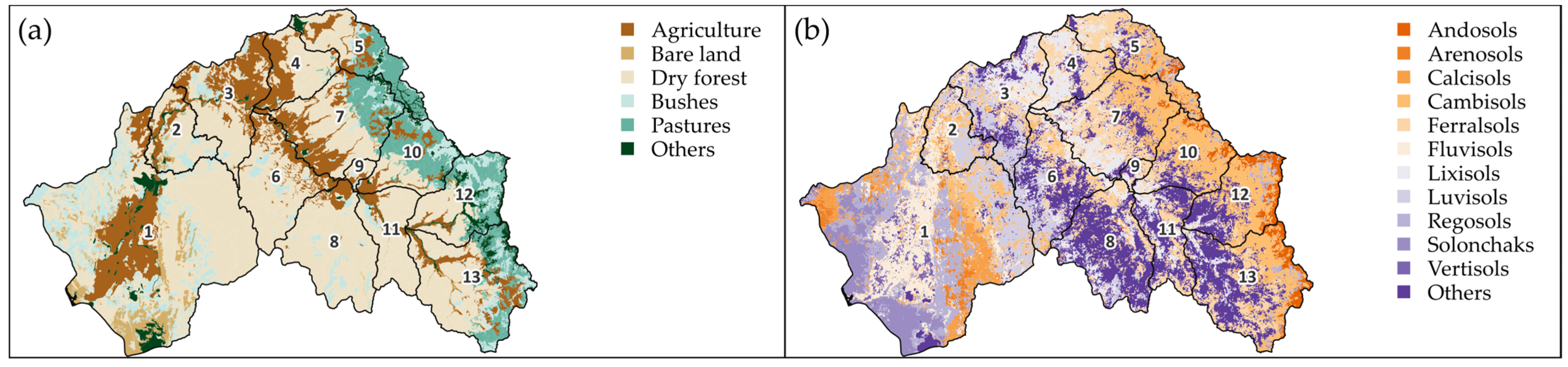
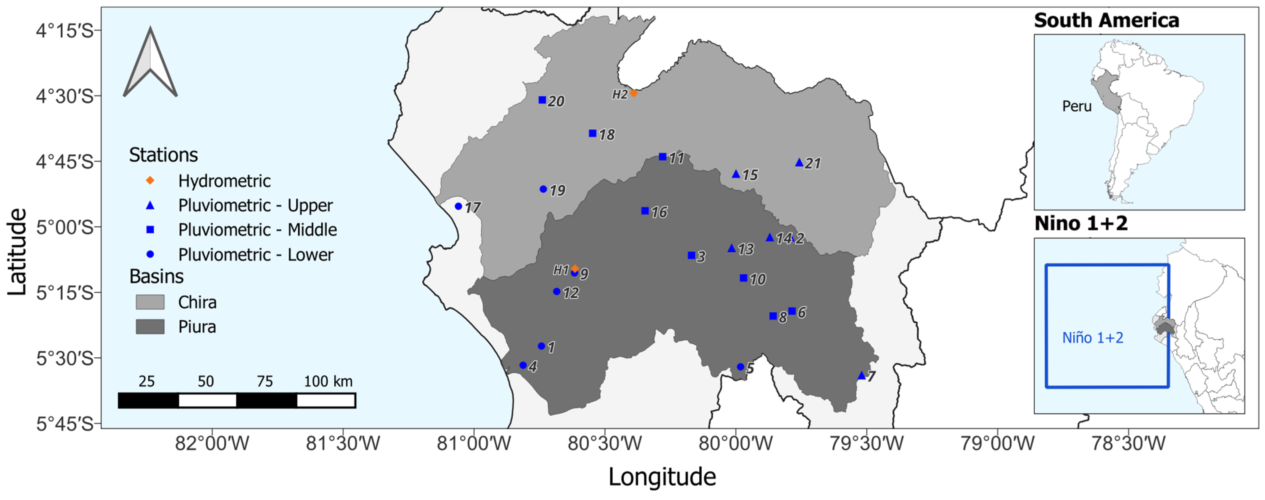
2.1. Study Area

The Piura River Basin (PRB) is situated in the Piura region, in the northwest of the Peruvian territory, along the western coast of South America (4°39′–5°43′ S and 81°03′–79°27′ W), with an area of 11.5 × 10³ km², draining from the Andes into the Pacific Ocean (Figure 1). The PRB may be divided into 3 zones according to altitude: upper, middle, and lower river basins. The upper river basin comprises around 30% of the PRB, and is located in the Andean zone, with peaks of up to 3700 m a.s.l. The middle river basin encompasses approximately 38% of the PRB, with altitudes between 80 and 400 m a.s.l. The remaining zone corresponds to the lower river basin, in the Sechura Desert, a flat and arid zone below 80 m a.s.l. This part of the mountain range is the lowest in South America, after Patagonia and Tierra del Fuego [18]. Based on the Pfafstetter coding system [19], the PRB is divided into nine hydrographic units (HUs). However, in our study, we adjusted the original division and obtained a total of 13 HUs as follows (

Table 1. List of the 3 subbasins and the 13 hydrologic units (HUs) into which the Piura River Basin is divided.

Subbasin	HU	Name	Subbasin	HU	Name
Lower	1	Bajo Piura	Middle	4	San Francisco
	2	Los Ejidos		6	Margen Izquierda
	3	La Penita		7	Margen Derecha
Upper	5	Chipillico		8	La Matanza
	12	Bigote		9	Medio Piura
	13	Alto Piura		11	Medio Alto Piura
	10	Corrales

). The Bajo Piura HU (Pfafstetter code 13781) was subdivided into three subunits, since it accounts for 41% of the PRB and it includes two critical points: the Los Ejidos hydrometric station and a proposed location for a new reservoir called La Peñita. The Medio Bajo Piura HU (Pfafstetter code 13784) exhibits contrasting physiographic characteristics across the banks of the Piura River, with desert on the left bank and dry forest on the right, so it was divided into two HUs. Lastly, the Chipillico HU (Pfafstetter code 13818), which belongs to the neighboring Chira basin, was included due to its hydrological interconnection with the Piura River. We believe these adjustments were necessary for accurate modeling.

According to Koppën’s classification, the climate of the PRB mainly corresponds to warm, arid, and semi-arid climate and according to Thornthwaite, arid climate prevails, being warm or temperate, with low humidity all year round. This kind of climate is characterized by moderate rainfall and high temperatures, with small seasonal fluctuations [20]. On the other hand, this arid climate is greatly modified by the presence of El Niño events. The northwest of the Peruvian territory is the zone most affected by El Niño, being subjected to the effect of the Humboldt cold current and the El Niño equatorial warm current. As Carrillo pointed out in 1892, in the Piura region, El Niño was recognized for the first time by fishermen at the Paita harbor [21].

Normal rainfall in the lower and middle subbasins of the PRB is scarce. In the capital city, Piura, the average rainfall, excluding El Niño years, is about 50 mm per year, while during the events of 1983 and 1998 it exceeded 2000 mm. This is also reflected in the great interannual variability around the whole PRB. In the lower river basin, the average annual rainfall is 200 mm (8 mm to 2300 mm), in the middle river basin it is 350 mm (13 mm to 3300 mm), and in the upper river basin it is 760 mm (200 mm to 2500 mm). The hydrological year in Peru goes from September to August, with maximum rainfalls from January to March. Figure 2a presents land cover of the Piura River Basin (PRB) that comprises approximately 51% dry forest, 14% agricultural land near the main course of the Piura River, and another 14% fallow land, predominantly located in the southern area corresponding to the Sechura Desert [22]. At the headwaters of UHs 5, 7, 10, 12, and 13, there is a pasture area that accounts for 8% of the PRB. Figure 2b presents a soils map of the PRB [23], the predominant soils are cambisols (22%) located at the headwaters of UHs 5, 7, 10, 12, and 13; ferrasols (20%) in UHs 4, 7 and 9; luvisols (10%) near the middle course of the river; and fluvisols (10%) around the lower course.

2.2. Data

2.2.1. Climatic Indices

Oceanic–atmospheric interaction influences the rainfall and flows observed in a region. To evaluate El Niño occurrence in northern coast of Peru, one atmospheric index and four climatic indices have been evaluated for the period 1950–2023. On the Tropical Pacific, the atmospheric anomaly was evaluated using the Southern Oscillation Index (SOI), which is a standardized index based on the difference in atmospheric pressures between Tahiti and Darwin, Australia [24]. Prolonged periods of negative (positive) SOI values coincide with abnormal warming (cooling) of the Tropical Pacific, typical of El Niño (La Niña), phases of ENSO. SOI data are published monthly by the US National Oceanic and Atmospheric Administration-NOAA Climate Prediction Center [25].

The SST is monitored in the Pacific Ocean by the NOAA. Currently, the main monitoring regions are two combinations of the four original ones. Niño 1 + 2 region (0°–10° S and 90° W–80° W) corresponds to the coastal region of South America and Niño 3.4 region is located in the central Pacific Ocean (5° N–5° S and 170° W–120° W) [26]. The first climatic indices are the Oceanic El Niño Index (ONI) and Coastal El Niño Index (CNI), which consist of the quarterly moving average of the SST anomaly in Niño 3.4 and Niño 1 + 2 regions, respectively, using climatology from the extended reconstructed product of monthly 2.0° × 2.0° SST, ERSSTv5 [27]. ONI is published monthly by CPC NOAA [25], and the neutral condition threshold is ±0.5 °C. CNI is published by IGP [28], and the neutral condition threshold is from −1 °C to 0.4 °C [29].

The other two climatic indices are the Coastal Laboratories Index (LABCOS) and the Peruvian coastal thermal index (PCTI), from Instituto del Mar del Perú (IMARPE); they evaluate the climatic behavior of the Peruvian coastal zone. LABCOS is a statistical indicator that reflects the amplitude of the variability of the SST in 6 IMARPE coastal stations (5° S–17° S), with the neutral condition threshold from −0.78 °C to +0.27 °C [30]. PCTI is calculated as the quarterly moving average of the reduced first component (CP1) (i.e., CP1 is divided by its standard deviation) of a principal component analysis of the SST anomalies at the Peruvian Upwelling Ecosystem zone. The neutral condition threshold goes from −0.78 °C to +0.27 °C [31].

2.2.2. Hydrometeorological Data

The time series of daily rainfall data (mm) recorded in the PRB from 1964 to 2023 by 16 meteorological stations were analyzed for space-time variability. To evidence El Niño occurrences during the same period, daily rainfall data (mm) recorded in the Chira River basin (CRB) were also included (

Table 2. List of the 21 rainfall stations used in this study. Asterisks indicate stations used only for El Niño analysis. Double asterisks indicate stations located in hydrological units of the upper river basin but considered in the middle river basin due to their altitude.

N°	Meteorological	Subbasin	River	Altitude	N°	Meteorological	Subbasin	River	Altitude
	Station		Basin	(m a.s.l.)		Station		Basin	(m a.s.l.)
1	Bernal	Lower	Piura	11	11	Partidor	Middle	Piura	254
2	Chalaco	Upper	Piura	2290	12	San Miguel	Lower	Piura	24
3	Chulucanas	Middle	Piura	89	13	San Pedro	Upper	Piura	240
4	Chusís	Lower	Piura	8	14	Santo Domingo	Upper	Piura	1490
5	El Virrey	Lower	Piura	211	15	Sapillica	Upper	Chira	1406
6 **	Hacienda Bigote	Middle	Piura	198	16	Tambogrande	Middle	Piura	60
7	Huarmaca	Upper	Piura	2171	17 *	La Esperanza	Lower	Chira	12
8	Malacasí	Middle	Piura	153	18 *	Lancones	Middle	Chira	133
9	Miraflores	Lower	Piura	34	19 *	Mallares	Lower	Chira	45
10 **	Morropón	Middle	Piura	128	20 *	Pananga	Middle	Chira	360
					21 *	Sausal de Culucán	Upper	Chira	980

).

The hydrometric records of the Piura and Chira River Basins were also evaluated (Figure 3). The data was obtained from the website of Servicio Nacional de Meteorología e Hidrología del Peru (SENAMHI) [32].

2.2.3. High-Resolution Gridded Rainfall Dataset—PISCO

PISCO (Peruvian Interpolated data of SENAMHI’s Climatological Observations) [33] is a meteorological gridded product developed for the Peruvian domain. It has the subproduct PISCOp v2p1, which contains a dataset with a daily rainfall at 0.1° spatial resolution (1981–2016). In this study, the time series of daily rainfall data from PISCO were obtained by means of ANDREA, the interactive platform of the National Water Resources Information System [34]. Data downloaded consisted of two types: data for the same location as SENAMHI meteorological stations and mean areal series for each of the 13 HU.

2.2.4. CMIP6 GCM

To evaluate future trends of the rainfall, this study utilized 20 CMIP6 GCMs (

Table 3. List of the 20 CMIP6 GCMs used in this study. Asterisk indicates the subset of models selected for further analysis.

N°	GCM Name	Institution	Country	Spatial Resolution lat° × lon°
1	ACCESS-CM2 *	CSIROARCCSS	Australia	1.875° × 1.25°
2	CanESM5	CCCma	Canada	2.8125° × 2.79°
3	CESM2 *	NCAR	USA	1.25° × 0.9424°
4	CESM2-WACCM *
5	CMCC-ESM2	CMCC	Italy
6	CNRM-CM6-1	Centre National de Recherches Météorologiques	France	1.25° × 1.25°
7	CNRM-ESM2-1			1.25° × 1.25°
8	EC-Earth3 *	International Centre for Earth Simulation	Norway	1.0° × 1.0°
9	EC-Earth3-Veg-LR *	EC—Earth Consortium	Europe	1.125° × 1.121°
10	HadGEM3-GC31-LL *	Met Office Hadley Centre	United Kingdom	1.25° × 1.25°
11	INM-CM4-8	INM	Rusia	2° × 1.5°
12	INM-CM5-0 *
13	MIROC6 *	MIROC	Japan	1.4° × 1.4°
14	MIROC-ES2L			1.406° × 1.406°
15	MPI-ESM1-2-HR	Max Planck Institute for Meteorology	Germany	0.6° × 0.6°
16	MPI-ESM1-2-LR			1.875° × 1.875°
17	MRI-ESM2-0	Meteorological Research Institute	Japan	1.125° × 1.125°
18	NESM3	University of Bergen and Norwegian Climate Centre	Norway	1.0° × 1.0°
19	NorESM2-LM *	Norwegian Climate Centre		2.5° × 1.89°
20	NorESM2-MM *			1.25° × 0.94°

) whose predictions are available and were accessed by Google Earth Engine with the “NEX-GDDP-CMIP6: NASA Earth Exchange Global Daily Downscaled Climate Projections” option. Daily rainfall for each of 13 HU was downscaled [35] and then analyzed using an multi-model ensemble average [11,36,37] of the 4 models with rainfall estimates for the future period (2023–2100) under two Shared Socioeconomic Pathways (SSP2-4.5 and SSP5-8.5) to assess the trend of projected rainfall over the study area [36]. The 4 best models were selected based on performance metrics [36,38] relative to the reference period (1981–2014).

2.3. El Niño Events Determination and Qualification

Based on data availability, the variability and behavior of the climatic indices were evaluated for the period 1950–2023. The analysis focused on the rainiest Peruvian season: from December to May. NOAA considers ENSO conditions to be present when the ONI is above or below the ±0.5 °C for a minimum of 5 consecutive months [26]. In this study, anomalous events were defined as those with 3 or more consecutive months of indices outside the normal range. This adjustment was made because, outside of the rainy season, ENSO does not significantly impact rainfall, floods, or overflows, and because Coastal El Niño events tend to be shorter in duration, typically lasting only two or three months. The analysis began with ONI and SOI to evaluate the coincidence of thermal and atmospheric anomalies, respectively, and to detect the years with El Niño (EN) or La Niña (LN) phases of ENSO in the central Pacific. The same criteria were applied for CNI, LABCOS, and PCTI to identify the years with warm (EN) and cold (LN) climatic anomalies recorded on the Peruvian coast.

Subsequently, the events identified on the Peruvian coast and in the central Pacific were compared to identify the nature of these anomalies, global or coastal. The coincidence of the type of anomaly, warm/cold, in a year denotes that the event perceived on the Peruvian coast was an ENSO, so we have Global El Niño (GEN)/Global La Niña (GLN). The discrepancy indicates the occurrence of warm/cold anomalies circumscribed to the Peruvian coast: Coastal El Niño (CEN)/Coastal La Niña (CLN). The effects caused by each event of climatic anomaly vary in magnitude, duration and spatial extension. In this work, we analyze the events according to how they have been perceived in the Piura region, which is the most affected by El Niño, to classify them by intensity. The categories of “very strong”, “strong”, “moderate”, and “weak” were considered for both types of anomalies, cold and warm, independently of its origin. To compare the effects perceived, the qualitative categories were converted to numerical values from −4, in very strong cold, to +4 in very strong warm.

To evaluate El Niño intensity, Farias and Montero [39] analyzed the annual maximum flow and transported volume of the Piura and Chira River Basins. In this study, the monthly maximum daily rainfall from December to May at 21 meteorological stations in the Piura Region was added as a criterion for evaluating intensity. Missing data in the original daily rainfall records from these stations were filled using linear regression with data from neighboring stations on the same dates. To assess the intensity of El Niño, the rainfall anomalies it produces must be quantified. The anomaly at each rainfall station was calculated by standardizing the monthly maximum daily precipitation values, dividing each value by the corresponding long-term monthly mean. These standardized values were then averaged across the three zones: lower, middle, and upper (Table 2), yielding a single standardized value for each month and year for each zone. The standardized values were subsequently converted into an integer index, denoted as the P_index, ranging from −4 to +4. This index represents conditions from drier (−4) to wetter (+4), with zero indicating neutral conditions. The calculation of the monthly P_index required defining the range of standardized rainfall corresponding to neutral conditions, which varies across zones (

Table 4. Threshold values for assigning P_index and categorizing climate anomalies based on standardized maximum daily rainfall quartiles in the lower, middle, and upper zones of the Piura region. EN: El Niño, LN: La Niña.

EN/LN Category	P_Index	Lower Zone	Middle Zone	Upper Zone
Very strong: EN4	+4	6.26–31.44	4.32–19.07	2.19–5.22
Strong: EN3	+3	3.88–6.26	2.87–4.32	2.00–2.19
Moderate: EN2	+2	2.80–3.88	2.25–2.87	1.83–2.00
Weak: EN1	+1	2.13–2.80	2.00–2.25	1.71–1.83
Neutral	0	0.30–2.13	0.50–2.00	0.90–1.71
Weak: LN1	−1	0.15–0.30	0.27–0.50	0.75–0.90
Moderate: LN2	−2	0.08–0.15	0.13–0.27	0.62–0.75
Strong: LN3	−3	0.02–0.08	0.05–0.13	0.49–0.62
Very strong: LN4	−4	<0.02	<0.05	0.09–0.49

Note: Color in the Category column represents the diverse kinds of anomalies.

). These ranges were determined based on the occurrence of anomalies in the ocean–atmospheric indices. Anomalies exceeding the neutral range were classified as humid and assigned a P_index from +1 to +4 depending on the quartile in which they fell. Conversely, anomalies below the neutral range were classified as dry and assigned a P_index from −1 to −4. The thresholds defining these categories are presented in Table 4. Finally, to characterize each hydrological year, a unique pair of extreme P_index values (minimum and maximum) were identified for the December-to-May period across the three zones of the Piura region. These values reflect the yearly minimum and maximum rainfall intensities.

Similarly, the annual maximum daily streamflow and annual volume records of the PRB and CRB were obtained. Next, the thresholds for these climatic and hydrometeorological indices were determined by calculating quartiles (

Table 5. Threshold values for assigning intensity indices and categorizing climate anomalies based on the extreme Coastal El Niño Index (CNI), annual maximum streamflow, and volume of Piura and Chira Rivers.

Categories	Index	CNI Ext (°C)	Streamflow Piura (m3/s)	Streamflow Chira (m3/s)	Volume Piura (hm3)	Volume Chira (hm3)
EN4	4	> 3.0	2652–3900	3255–8000	3510–14,049	7081–18,164
EN3	3	1.7–3.0	1747–2652	2577–3255	2066–3510	6291–7081
EN2	2	1.0–1.7	1513–1747	2207–2577	1659–2066	4983–6291
EN1	1	0.4–1.0	1000–1513	1654–2207	1240–1659	3743–4983
Neutral	0	−1.0–0.4	350–1000	798–1654	624–1240	3615–3743
LN1	−1	−1.2–−1.0	122–350	578–798	420–624	2148–3615
LN2	−2	−1.4–−1.2	74–122	405–578	204–420	1737–2148
LN3	−3	−2.0–−1.4	34–74	307–405	83–204	1358–1737
LN4	−4	<−2.0	0–34	150–307	0–83	767–1358

Note: Color in the Categories column represents the diverse kinds of anomalies.

). Finally, the indices from Table 4 and Table 5 were averaged for each year and allowed to classify the events that occurred on the Peruvian coast between 1950 and 2024.

2.4. Spatial Variability of Maximum Daily Rainfall

To assess the spatial variability of maximum daily rainfall, isohyet maps were produced for the entire basin based on data from the meteorological network stations for statistical indices and various El Niño scenarios. The point format data was interpolated with the QGIS 3.32.3 [40] using the v.surf.rst tool of GRASS GIS v.8.4.0RC1 [41], which performs surface interpolation from vector points map to floating point raster format using regularized spline with tension [42,43]. This method was selected over Inverse Distance Squared Weighting due to its ability to produce smoother and more continuous surface representations.

2.5. Temporal Variability of Maximum Daily Rainfall

To assess the temporal trend in annual maximum daily rainfall, the Mann–Kendall (MK) test [44,45,46,47,48,49] was used. This is a non-parametric test based on the sequential comparison of the values of a time series, considering the hypothesis of stability of the series. Koudahe et al. [48] highlight that the MK test statistic is dimensionless and does not offer a quantification of the trend in the units of the time series under study, but rather offers information about the direction and a measure of the importance of the observed trends. For series longer than 10 years, the MK test statistic Z approximately follows a standard normal distribution. The null hypothesis for this test is that there is no trend in the series. This is accepted if $\left|Z\right|<\left|Z_{1-\alpha /2}\right|$ at the significance level of α < 5% [37,49], that is the 97.5%-quantile in the standard normal distribution. The +/− sign of Z indicates an increasing/decreasing trend in the series. The implementation process of the MK test is detailed by Li et al. [46]. The analysis was carried out with the free software TREND v.1.0.2 [50] to identify the series where climate variability and the effect of El Niño are significant. To quantify the magnitude of trend, Sen’s slope method [51,52,53,54,55] was used. This estimator is unbiased and is determined with the median of the set of slopes that join pairs of values in the series:

$$\beta =median\left({\displaystyle \frac{x_i-x_j}{i-j}}\right),\forall j<i$$

(1)

where x_i and x_j are the data values at years i and j. The resulting slope is in mm/year.

Another sign of temporal variability in data is when it denotes a shift. The Cusum test [56,57,58,59] is a non-parametric test that evaluates whether the mean of the time series presents a significant shift in value and determines the year in which the change occurs. The process to calculate the Cusum test statistic V_k is detailed by Hallouz et al. [57]. The null hypothesis for this test is that there is no shift in the series. Critical values of $\left|V_k\right|$ at 5% and 1% significance levels are 1.36$\sqrt{n}$ and 1.63$\sqrt{n}$, respectively. If calculated $\left|V_k\right|$ exceeds the critical values, it is accepted that the series presents a statistically significant shift [60].

2.6. GCMs Downscaling and Performance Metrics

GCMs provide reliable predictions at large scales; however, they still need to be corrected by downscaling [11,37,61,62]. Downscaling techniques encompass a broad set of procedures aimed at improving GCM predictions for various climate studies. Some focus on the spatial dimension, enhancing spatial resolution or correcting biases, while others target improvements in the temporal scale [37,61]. This study uses daily GCM simulations at subbasin or hydrological unit levels, so only bias correction was necessary. The linear scaling method [35,61,63] is a statistical approach that corrects GCM biases by identifying the relationships between large-scale climate patterns and local climate responses observed on a monthly basis. For rainfall predictions, these relationships are applied to GCM daily predictions, $P_{GCM}^{m,d}$, using a monthly multiplicative correction factor. This factor is calculated by comparing the average of observed data (i.e., PISCO gridded dataset) and GCM historical simulations during the reference period (1981–2014). Thus, statistically adjusted products, $P_{GCMadj}^{m,d}$, were obtained for the GCM daily predictions [35]:

$$P_{GCMadj}^{m,d}=P_{GCM}^{m,d}\left[{\displaystyle \frac{{\overline{P}}_{obs}^m}{{\overline{P}}_{GCMhist}^m}}\right]$$

(2)

Then, the performance of GCMs was evaluated by comparing historical simulations with the PISCO gridded dataset, using performance metrics to select a subset of the best-performing models [11,36,37,43,64]. Bağçaci et al. [36] recommend applying at least one goodness-of-fit measure and at least one absolute error measure. Thus, the modified agreement index (md) and normalized root mean square error (nRMSE) were used. Each of these metrics allowed the creation of a ranking of models, from 1 to 20, and the average of both rankings determined the top four GCMs, similar to the comprehensive rating index MR proposed by Jiang [65]. A multi-model ensemble average (MMEA) [11,36,37] was then constructed for each HU, considering the predictions of the top four GCMs [36].

Legates and McCabe [66] proposed a modified agreement index based on Willmott’s [67] agreement index for the validation of hydrological and hydroclimatic models, which represents the relationship between the mean square error and the potential error. Bağçaci et al. [36] named it md:

$$md=1.0-{\displaystyle \frac{{\sum }_{i=1}^n\left|O_i-P_i\right|}{{\sum }_{i=1}^n\left(\left|P_i-\overline{O}\right|+\left|O_i-\overline{O}\right|\right)}}$$

(3)

where P are the predictions of each GCM, and O are the observations (here, the PISCO gridded dataset). The md varies between 0 (no match) and 1 (perfect match). Its advantage is that errors and differences receive appropriate weighting and are not inflated by quadratic values [66]. Bağçaci et al. [36] indicate that the normalized root mean square error (nRMSE) has an advantage over RMSE in evaluating model performance when the variables are in different orders of magnitude and follows the normalization process given by Almeida et al. [38], where lower nRMSE values indicate less residual variance and therefore better model performance:

$$nRMSE={\displaystyle \frac{{\left[\frac{1}{n}{\sum }_{i=1}^n{\left(P_i-O_i\right)}^2\right]}^{1/2}}{O_{max}-O_{min}}}$$

(4)

3. Results

3.1. El Niño Events in Piura Region

A period of 75 hydrological years (1949/50–2023/24) was analyzed, during which the values of climatic and atmospheric indices were compared for the El Niño 1 + 2 and El Niño 3.4 regions. Approximately 49% of the years were classified as either El Niño or La Niña events, occurring at both global and coastal scales. Additionally, using predefined thresholds, the intensity of these events was identified (Figure 4), and their incidence and return periods were calculated (

Table 6. Identification of anomalous hydrological years in the Piura region by intensity and determination of return periods (1950–2024). Bold years are from the recent 30-year period (1993–2023) and italic and underlined years are from the older 30-year period (1963–1993) discussed below.

Category	Hydrological Years				Total and Incidence	Total by Intensity				Return Period (Years)
	EN1/LN1	EN2/LN2	EN3/LN3	EN4/LN4		1 to 4	2 to 4	3 to 4	4	EN1/LN1	EN2/LN2	EN3/LN3	EN4/LN4
Global El Niño	1957–58	2015–16	1952–53	1982–83	10; 13%	19	10	8	3	4.0	7.6	9.5	25.3
	1986–87		1991–92	1997–98
	1992–93
	2018–19
	2023–24
Coastal El Niño	1956–57	1971–72	2001–02	2016–17	9; 12%
	1964–65		2007–08
	1996–97		2022–23
	2011–12
Global La Niña	1954–55	1970–71	1973–74	1949–50	12; 16%	18	15	10	4	4.2	5.1	7.6	19.0
	1955–56	2010–11	1984–85	1967–68
	2020–21	2021–22	1995–96
			2017–18
Coastal La Niña		1961–62	1953–54	1963–64	6; 8%
		1980–81	2012–13	1965–66
Neutral *	1950–51	1974–75	1988–89	2004–05	38; 51%	38				2.0
	1951–52	1975–76	1989–90	2005–06
	1958–59	1976–77	1990–91	2006–07
	1959–60	1977–78	1993–94	2008–09
	1960–61	1978–79	1994–95	2009–10
	1962–63	1979–80	1998–99	2013–14
	1966–67	1981–82	1999–00	2014–15
	1968–69	1983–84	2000–01	2019–20
	1969–70	1985–86	2002–03
	1972–73	1987–88	2003–04

Note: * Neutral years do not have intensity. Color in the Category column represents the diverse kinds of anomalies.

).

The incidence of warm anomalies is almost equal to that of cold ones, at 25% and 24%, respectively. The highest incidence corresponds to global events, at 29%, compared to 20% for coastal events. The return period for weak events (EN1/LN1) was around 4.1 years, while for moderate events (EN2/LN2) it was about 6.4 years, and for strong events (EN3/LN3) it was approximately 8.5 years for both warm and cold anomalies. In the case of very strong events, EN had a return period of 25 years, while LN had a return period of 19 years. Normal or neutral years, i.e., without anomalies, had a 2-year return period, corresponding to an incidence of 51%.

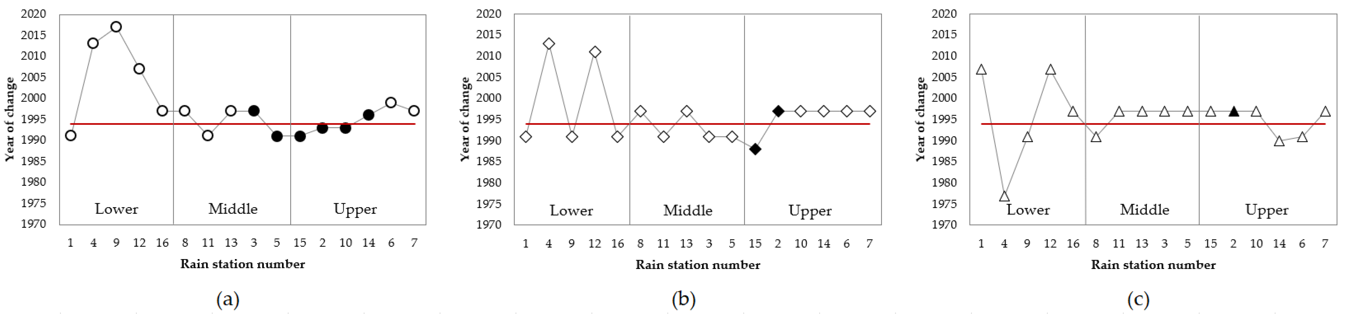
3.2. Temporal Variability

The temporal trend of rainfall in the Piura River Basin (PRB) was analyzed using the Mann–Kendall (MK) test on the 60-year series (1963/64–2022/23) from 16 stations in the SENAMHI network. The results are shown in Figure 5 for annual maximum daily rainfall (Figure 5a), annual maximum monthly rainfall (Figure 5b), and annual rainfall (Figure 5c) at the same stations. In general, the lower basin of the PRB did not show a significant trend, except for the Tambogrande station (16). In contrast, the middle basin predominantly exhibited a significant positive trend, except at the Partidor station (11). In the upper basin, all stations showed a significant positive trend at the daily level, but the Santo Domingo station (14) did not exhibit this trend when analyzing monthly rainfall. In addition, at the annual level, the Chulucanas (3), Huarmaca (7), and Sapillica (15) stations did not show significant trends.

The Cusum test was applied to the same rainfall series on the three timescales. The results are shown in Figure 6. At the daily scale (Figure 6a), only parts of the middle and upper basins exhibited significant changes, while at the monthly (Figure 6b) and annual (Figure 6c) scales, there was no significant change in almost all stations. Despite this, the year 1994 appeared to be the average year for some change across all three timescales. Subsequently, spatial variability was analyzed for two periods: 1963–1993 and 1993–2023.

Figure 7 shows the results of the MK test applied to the series of maximum daily rainfall from the PISCO gridded dataset and the GCMs at the HU level. The historical series from both PISCO and the GCMs showed no significant trends, except for HU10 in the PISCO gridded dataset. Comparing this with Figure 5a, we can deduce that the data from the SENAMHI network shows a more significant trend than the PISCO and GCM data. A reason for this disparity may lie in the different length of the series analyzed; the PISCO gridded dataset has 36 years of records and the historical GCMs have 34 years of predictions, while the SENAMHI network data are 60 years long. On the other hand, the projected series under the SSP2-4.5 scenario indicates a significant increasing trend only in the southern middle and upper basin. Under the SSP5-8.5 scenario, a significant increasing trend is observed across the entire study area, according to these predictions.

Figure 8 shows the results of the Cusum test applied to the PISCO gridded dataset and GCMs series at the HU level. The PISCO and historical GCM series did not practically show significant changes (Figure 8a). In the projected series for future scenarios, the SSP2-4.5 scenario showed 4 HUs with significant changes, while SSP5-8.5 exhibited a significant change with an average occurrence around the year 2068 (Figure 8b).

Figure 9a shows the Sen’s slope calculated for the 60-years SENAMHI network series at three timescales, combined with the MK results from Figure 5a. The height of the bars represents the estimation of Sen’s slope, while their color (filled or empty) indicates the significance of the MK test. In general, the slopes at stations in the lower subbasin of the PRB are smaller and show no significant trend, except for the Tambogrande station (16), located in the rainiest area during El Niño events. At the daily and monthly maximum timescales, the largest slopes are observed in both the middle and upper subbasins of the PRB, while at the annual scale, the largest slopes are found in the upper subbasin. In this case, the reason may be that the rainy season lasts longer in the upper part of the basin than in the lower part. Figure 9b shows the analysis at the HU level. It is observed that the PISCO series presents greater slopes than the historical GCM series, although almost none are significant, except for HU10 in the upper zone for the PISCO series. In contrast, the slopes under the SSP5-8.5 scenario are markedly greater and more significant than those under SSP2-4.5.

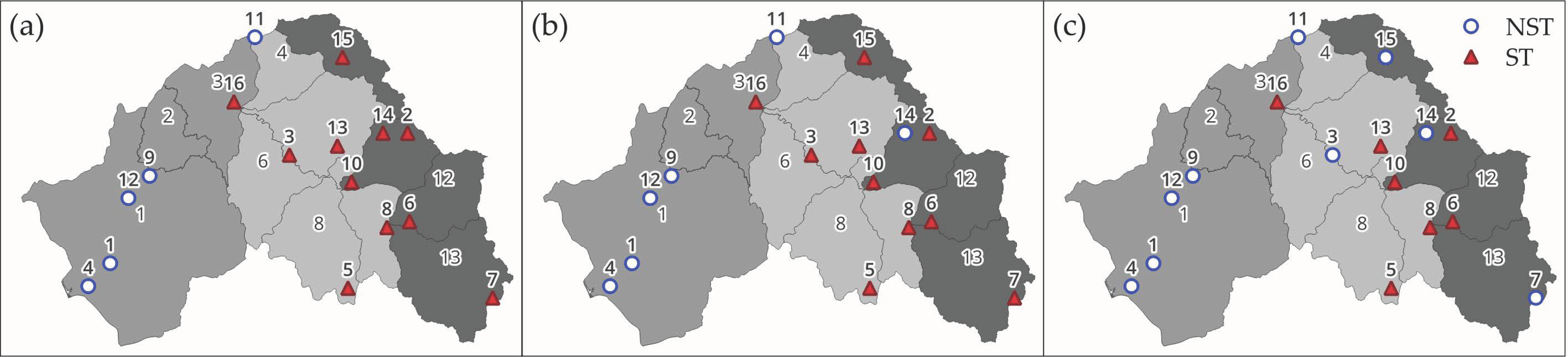
3.3. Spatial Variability

Figure 10 shows the results of the spatial variability analysis of the maximum daily rainfall recorded in PRB. In addition to the complete 60-year period (1964–2023), two 30-year periods were analyzed: the older series (1964–1993) and the recent series (1994–2023), based on the temporal variability results.

To better show the rainfall variation in the PRB across the Hus, isohyets have been included in the raster maps. In the complete series (Figure 10a), the greatest amount of rainfall (P > isohyet 60 mm) was concentrated around the upper and middle course of the river (HUs 13, 11, 10, 9, and 7). In the old series (Figure 10b), rainfall (P > 50 mm) was concentrated in HUs 13, 7, 9, and 10, while in the recent series (Figure 10c) rainfall (P > 80 mm) was highly concentrated in the middle course, specifically in HU 9. The historical extremes (Figure 10d,e) and the maximum standard deviation (Figure 10f), with isohyets 0 mm, 300 mm, and 60 mm, respectively, were concentrated in HU 8, a desert area that is highly affected by El Niño events. This confirms that HU 8 experiences the most extreme climate variability due to El Niño. Regarding the distribution during El Niño years (Figure 10i–l), when analyzing neutral years (Figure 10g) and La Niña years (Figure 10h), the isohyets showed a similar distribution of maximum daily rainfall, with P > 50 mm centered on the head of the basin (HU 13) and on the right bank of the middle basin (HUs 7 and 10). During EN1 (Figure 10i), the maximum daily rainfall was centered on the south, HUs 8, 11, and 13, with P > 80 mm, preserving, to some extent, the regular mountain rainfall patterns. In contrast, during EN2, EN3, and EN4, the pattern shifted (Figure 10j–l), with maximum daily rainfall mainly concentrating in the middle basin, in HUs 6, 8, and 9, where isohyets 80, 120, and 200 mm, respectively, are found.

Figure 11 condenses these findings from the daily scale analysis (Figure 11a) into a pair of linear graphs and complements them with the results at maximum monthly (Figure 11b) and annual (Figure 11c) timescales. In general, higher values were observed in the recent 30-year series (1994–2023) compared to the older one (1964–1993), with increases averaging 58%, 59%, and 46% on the daily, monthly, and annual scales, respectively. At the daily maximum scale (Figure 11a), the average rainfall values were similar in the middle and upper subbasins of the PRB, and lower in the lower subbasin. However, at the monthly maximum (Figure 11b) and annual scales (Figure 11c), the upper subbasin exhibited higher average values. The minimum values across all three timescales occurred in the lower and middle subbasins, while the largest standard deviations were concentrated in the middle zone, reflecting the transition from droughts to floods due to El Niño. The behavior of HU3 La Peñita, in the lower subbasin, was more like that of the middle subbasin, in terms of mean values and during El Niño events. The HUs most influenced by El Niño events were HU3, HU6, and HU8, particularly on the left bank. On a daily scale (Figure 11a), HU11 also showed extreme values. Generally, the behavior of neutral years and La Niña years were very similar, but El Niño patterns varied according to their intensity. During EN1, rainfall in the middle and lower subbasins did not exceed the usual rainfall in the upper subbasin. However, during EN2 and EN3, the daily maximum rainfall (Figure 11a) was concentrated in the middle subbasin, the monthly maximum rainfall (Figure 11b) was similar in both the middle and upper subbasins, but the annual totals (Figure 11c) were still higher in the upper subbasin. During very strong events, EN4, the lower and middle subbasins exceeded the upper subbasin across all three timescales.

4. Discussion

This study analyzed the space-time variability of maximum daily rainfall in the Piura River Basin, located on the northern coast of Peru, in relation to El Niño occurrence. We identified and classified El Niño and La Niña events based on their intensity, evaluated the spatiotemporal variability of maximum daily rainfall, and assessed the predictions from CMIP6 GCMs. Our classification of EN/LN events revealed significant variability in both intensity and frequency throughout the study period. A clear distinction between global and coastal events was observed, with the latter having a more localized impact on the PRB.

The spatiotemporal variability analysis revealed distinct patterns in maximum daily rainfall across the hydrologic units of the PRB. The lower basin exhibited greater rainfall variability, particularly during El Niño years, while the upper basin showed a more stable rainfall pattern. Rainfall in the middle basin was influenced by dynamics from both the upper and lower basin. CMIP6 GCM projections suggested an overall increase in maximum daily rainfall in the future, with significant implications for flood risk and water resource management. Although the performance varied across models, the multi-model ensemble average approach provided robust projections for the PRB.

Our findings align with previous studies highlighting the impact of ENSO events on rainfall variability in the region. However, our research advances this understanding by differentiating between global and coastal EN events and their specific impacts on the PRB. This distinction is crucial for accurate climate impact assessments and planning. The results emphasize the importance of incorporating ENSO diversity into climate impact assessments. For flood management and infrastructure planning, understanding the distinct impacts and predictability of global and coastal EN events can guide the design of resilient infrastructure. These findings also carry significant implications for agriculture and water resource management, given the region’s reliance on rainfall patterns.

This study faced several limitations, including the sparse density of the meteorological network and the resolution of the GCMs. Future research should address these limitations by incorporating higher-resolution data and exploring additional climatic variables to better model the extreme floods and asses the socioeconomic implications of rainfall variability and extreme events in the PRB. Additionally, improving the accuracy of climate models and their projections for the region remains a priority.

4.1. Impact of the Recurrence of El Niño

A recent trend toward wetter conditions has been observed, marked by an increase in the recurrence of EN events, particularly coastal EN events. Over the last 30 years (1993–2023), nine EN events have been detected, six of which were CEN type. In contrast, during the previous 30-year period (1963–1993), only two CEN and four GEN events occurred. This rise in the frequency of CEN events is significant, signaling a shift in the climatic patterns affecting the PRB. The return period for EN events in general has decreased from 5.2 years to 3.4 years. In addition, when analyzing the average intensity indices of EN/LN events, which range from −4 to +4 (with 0 representing neutral years), it revealed that the intensity during anomalous years in the older period had an average value of −0.77, indicating a predominance of La Niña events. In contrast, the recent 30-year period has an average intensity of +0.53, confirming a higher frequency of warm El Niño events. This shift towards more frequent El Niño events, especially Coastal EN events, is crucial for understanding the changes in rainfall patterns in the PRB.

The most common climate anomalies perceived in Piura in this century XXI have been five CEN events, of which one was very strong, three were strong and one was weak. These events, combined with three GEN (one moderate and two weak), bring the total to eight EN events over the past 24 years. The recurrence of these events, approximately every three years, highlights a notable frequency that must be considered in regional planning and analysis.

However, when evaluated over the long term, considering the last century, the inclusion of 16 El Niño (EN) events identified in our study between 1950 and 2024 with the six events detected by Quinn et al. [7] between 1925 and 1949 results in a return period of approximately 4 years for warm events. Similarly, the specific return periods for strong and very strong EN events remain around 9 and 25 years, respectively.

The greater number of El Niño events in the recent period explains the observed increase in the average values of maximum daily rainfall across all stations in the PRB. The heightened recurrence of these warm events has led to more intense and frequent rainfall, contributing to the wetter conditions in the region. This trend has significant implications for flood risk management, agricultural planning, and water resource management, as the region must adapt to the increased rainfall variability and intensity. Furthermore, the shift towards more frequent and intense EN events is consistent with broader climatic trends reported in other studies, suggesting a possible link to global climate change. The implications of this shift are multifaceted. For instance, the increased frequency of extreme rainfall events could lead to more frequent flooding, presenting challenges for infrastructure and urban planning. This highlights the need for continuous monitoring and adaptive management strategies to mitigate the effects of these climatic changes on the PRB. However, wetter conditions could benefit agricultural activities, provided that appropriate water management practices are implemented to handle the variability.

Understanding the impacts of CEN versus GEN events, along with their predictability, is crucial for developing targeted mitigation and adaptation strategies. In Peru, the attention should not be solely focused on international ENSO predictions (i.e., NOAA). The localized and sudden nature of CEN events often leads to more intense effects in specific areas, requiring concentration in prevention and tailored responses to effectively manage the risks and leverage on potential benefits.

4.2. Change in Spatial Distribution Patterns of Rainfall in the Region

The spatial distribution of rainfall during EN events, particularly EN2 and EN3 events, shows significant variations compared to neutral years. The middle subbasin of the PRB, specifically HU6, experiences the highest rainfall intensities during these events. In the HU6, maximum daily rainfall reaches 303% and 367% of the average value during neutral years for EN2 and EN3 events, respectively. This substantial increase highlights the pronounced impact of these climatic anomalies on rainfall distribution patterns. Similar significant percentage variations are observed in HU2, located in the lower zone, typically dry. These findings indicate that the influence of El Niño events extends across various parts of the basin, altering the typical rainfall distribution patterns and increasing the risk of extreme rainfall events.

Given these observations, design rainfall calculations and water management strategies must not treat El Niño events as mere outliers. The high incidence and distinct rainfall distribution patterns during these events make their inclusion in hydrological models and infrastructure planning vital. Ignoring the impact of El Niño results in underestimating flood risks and inadequate preparation for extreme weather events. The frequent and intense rainfall associated with El Niño, particularly CEN events, calls for a reassessment of current hydrological designs and flood-management plans. Infrastructure must be designed to withstand the increased rainfall intensities observed during these periods to prevent damage and ensure resilience.

Figure 12 compares the behavior of the two types of El Niño events studied, in their different intensities, along the HUs of the PRB. The very strong global events have had greater intensity in almost the entire basin, except in HU5. For the rest of the intensities, the coastal events have been greater. In general, the rainiest area turns out to be the middle subbasin, but the relative change to the average of the neutral years is greater in the lower subbasin. It was also confirmed that in both cases, global and coastal, the upper subbasin is the one that sees its rainfall pattern altered the least.

4.3. Projections of General Circulation Models (GCMs)

The use of GCMs in the study provides critical insights into the future spatiotemporal variability of maximum daily rainfall in the PRB. Data from the top four performing GCMs were analyzed across the 13 HUs within the PRB. These models were selected based on their performance in simulating historical climate data, evaluated using two key metrics: the modified agreement index (md) and the normalized root mean square error (nRMSE). A multi-model ensemble average was created for each HU to project future climate scenarios and analyze potential trends in rainfall patterns. The GCM projections indicate significant changes in the spatial and temporal distribution of maximum daily rainfall in the PRB, aligning with the observed increase in El Niño events and their regional impact. These results underscore the need to incorporate projected changes in infrastructure planning and design. The high recurrence of El Niño events, combined with the GCM projections, suggests that future rainfall patterns may diverge significantly from historical norms, necessitating updated design standards to mitigate flood risks. While GCMs provide valuable projections, inherent uncertainties exist in climate modeling. This study addresses these uncertainties by using an ensemble approach, which averages the outputs of multiple models to reduce individual biases. The bias of the GCMs used in the study was corrected with the PISCO gridded dataset, a high-resolution gridded rainfall product specific to Peru. This local calibration not only enhances the reliability of the projections for the PRB, but also underscores the importance of region-specific data in climate studies.

5. Conclusions

It is confirmed that in the Piura region, and generally along the Peruvian coast, there is a distinct manifestation of El Niño separate from ENSO, which in its warm phase, is known as Coastal El Niño. This phenomenon has been notably recurrent if we focus on the recent 30-year period or even the present century and significantly alters the maximum daily, monthly, and annual rainfall values in the Piura River Basin. The increased recurrence of El Niño, particularly Coastal El Niño (CEN) events, has resulted in a substantial rise in maximum daily rainfall in the PRB over the past 30 years. This trend highlights the need for comprehensive and adaptive strategies to manage the associated risks and leverage potential opportunities in the context of climate change.

Although the rainfall record in the Piura River Basin is limited for assessing long-term climate change, the analysis of the recurrence of El Niño (EN) events revealed that the last 30 years have been more intense than the preceding 30 years. However, updating the results of Quinn et al. [7] to assess the past 100 years, the long-term recurrence remains similar to the 76-year series analyzed.

Furthermore, the spatial variability in rainfall patterns during El Niño events suggests that regional planning and resource allocation must be tailored to the specific conditions of each HU within the PRB. This approach ensures that areas most affected by extreme rainfall receive adequate attention and resources for flood prevention, mitigation, and water management. The changing spatial distribution of rainfall in the PRB, driven by the increasing frequency and intensity of El Niño events, highlights the need for comprehensive and adaptive water management strategies. By considering the unique impacts of these climate anomalies, planners and policymakers can better prepare for and mitigate the risks associated with extreme rainfall and flooding events, thereby ensuring population resilience and the sustainability of the region’s water infrastructure and resources.

References

1. McPhaden, M.J.; Zebiak, S.E.; Glantz, M.H. ENSO as an Integrating Concept in Earth Science. Science 2006, 314, 1740–1745. [Google Scholar] [CrossRef]
2. Cai, W.; Santoso, A.; Collins, M.; Dewitte, B.; Karamperidou, C.; Kug, J.-S.; Lengaigne, M.; McPhaden, M.J.; Stuecker, M.F.; Taschetto, A.S.; et al. Changing El Niño–Southern Oscillation in a Warming Climate. Nat. Rev. Earth Environ. 2021, 2, 628–644. [Google Scholar] [CrossRef]
3. McPhaden, M.J.; Santoso, A.; Cai, W. (Eds.) El Niño Southern Oscillation in a Changing Climate, 1st ed.; Geophysical Monograph Series; Wiley: Hoboken, NJ, USA, 2020. [Google Scholar] [CrossRef]
4. Takahashi, K. Fenómeno El Niño: “Global” vs “Costero”. In Boletín Técnico: Generación de Información y Monitoreo del Fenómeno El Niño, Instituto Geofísico del Perú; Instituto Geofísico del Perú: Lima, Peru, 2017; Volume 4, pp. 4–7. [Google Scholar]
5. Capotondi, A.; Wittenberg, A.T.; Kug, J.-S.; Takahashi, K.; McPhaden, M.J. ENSO Diversity. In El Niño Southern Oscillation in a Changing Climate; Geophysical Monograph Series; Wiley: Hoboken, NJ, USA, 2020; pp. 65–86. [Google Scholar] [CrossRef]
6. Capotondi, A.; Sardeshmukh, P.D. Is El Niño Really Changing? Geophys. Res. Lett. 2017, 44, 8548–8556. [Google Scholar] [CrossRef]
7. Quinn, W.H.; Neal, V.T.; Antunez De Mayolo, S.E. El Niño Occurrences over the Past Four and a Half Centuries. J. Geophys. Res. 1987, 92, 14449. [Google Scholar] [CrossRef]
8. Deser, C.; Wallace, J.M. El Niño Events and Their Relation to the Southern Oscillation: 1925–1986. J. Geophys. Res. Ocean. 1987, 92, 14189–14196. [Google Scholar] [CrossRef]
9. Takahashi, K. Física Del Fenómeno El Niño “Costero”. In Generación de Información y Monitoreo del Fenómeno El Niño; Instituto Geofísico del Perú: Lima, Peru, 2017; p. 16. [Google Scholar]
10. Sanabria, J.; Bourrel, L.; Dewitte, B.; Frappart, F.; Rau, P.; Solis, O.; Labat, D. Rainfall along the Coast of Peru during Strong El Niño Events. Int. J. Climatol. 2018, 38, 1737–1747. [Google Scholar] [CrossRef]
11. Almazroui, M.; Islam, M.N.; Saeed, F.; Saeed, S.; Ismail, M.; Ehsan, M.A.; Diallo, I.; O’Brien, E.; Ashfaq, M.; Martínez-Castro, D.; et al. Projected Changes in Temperature and Precipitation Over the United States, Central America, and the Caribbean in CMIP6 GCMs. Earth Syst. Environ. 2021, 5, 1–24. [Google Scholar] [CrossRef]
12. Ashfaq, M.; Ghosh, S.; Kao, S.; Bowling, L.C.; Mote, P.; Touma, D.; Rauscher, S.A.; Diffenbaugh, N.S. Near-term Acceleration of Hydroclimatic Change in the Western U.S. JGR Atmos. 2013, 118, 10676–10693. [Google Scholar] [CrossRef]
13. Batibeniz, F.; Ashfaq, M.; Diffenbaugh, N.S.; Key, K.; Evans, K.J.; Turuncoglu, U.U.; Önol, B. Doubling of U.S. Population Exposure to Climate Extremes by 2050. Earth’s Future 2020, 8, e2019EF001421. [Google Scholar] [CrossRef]
14. Rastogi, D.; Touma, D.; Evans, K.J.; Ashfaq, M. Shift Toward Intense and Widespread Precipitation Events Over the United States by Mid-21st Century. Geophys. Res. Lett. 2020, 47, e2020GL089899. [Google Scholar] [CrossRef]
15. Taylor, K.E.; Stouffer, R.J.; Meehl, G.A. An Overview of CMIP5 and the Experiment Design. Bull. Am. Meteorol. Soc. 2012, 93, 485–498. [Google Scholar] [CrossRef]
16. Eyring, V.; Bony, S.; Meehl, G.A.; Senior, C.A.; Stevens, B.; Stouffer, R.J.; Taylor, K.E. Overview of the Coupled Model Intercomparison Project Phase 6 (CMIP6) Experimental Design and Organization. Geosci. Model. Dev. 2016, 9, 1937–1958. [Google Scholar] [CrossRef]
17. WCRP. CMIP Phase 6 (CMIP6)-Coupled Model Intercomparison Project. Available online: https://wcrp-cmip.org/cmip6/ (accessed on 21 June 2024).
18. De Reparaz, G. Los Ríos de la Zona Árida Peruana; Universidad de Piura: Piura, Peru; ICC: Barcelona, Spain, 2013. [Google Scholar]
19. Autoridad Nacional del Agua. Delimitación y Codificación de Unidades Hidrográficas del Perú; Memoria descriptiva; Autoridad Nacional del Agua: Lima, Perú, 2012; p. 104.
20. Autoridad Nacional del Agua. Plan de Gestión de los Recursos Hídricos de la cuenca Chira-Piura; Autoridad Nacional del Agua: Lima, Perú, 2015.
21. Woodman, R.; Takahashi, K. ¿Por qué no llueve en la costa del Perú (salvo durante El Niño)? Boletín Técnico 2014, 1, 4–7. [Google Scholar]
22. Gobierno Regional de Piura. La. Zonificación Ecológica Económica de La. Región Piura; Gobierno Regional de Piura: Lima, Perú, 2012.
23. Batjes, N.H.; Calisto, L.; De Sousa, L.M. Providing Quality-Assessed and Standardised Soil Data to Support Global Mapping and Modelling (WoSIS Snapshot 2023). Earth Syst. Sci. Data 2024, 16, 4735–4765. [Google Scholar] [CrossRef]
24. Trenberth, K.E. Signal versus Noise in the Southern Oscillation. Mon. Weather Rev. 1984, 112, 326–332. [Google Scholar] [CrossRef]
25. CPC NOAA. Climate Prediction Center-Monitoring & Data: Current Monthly Atmospheric and Sea Surface Temperatures Index Values. Available online: https://www.cpc.ncep.noaa.gov/data/indices/ (accessed on 25 March 2023).
26. Trenberth, K.E. The Definition of El Niño. Bull. Am. Meteorol. Soc. 1997, 78, 2771–2778. [Google Scholar] [CrossRef]
27. Huang, B.; Thorne, P.W.; Banzon, V.F.; Boyer, T.; Chepurin, G.; Lawrimore, J.H.; Menne, M.J.; Smith, T.M.; Vose, R.S.; Zhang, H.-M. Extended Reconstructed Sea Surface Temperature, Version 5 (ERSSTv5): Upgrades, Validations, and Intercomparisons. J. Clim. 2017, 30, 8179–8205. [Google Scholar] [CrossRef]
28. IGP. Datos ICEN. Available online: http://met.igp.gob.pe/datos/icen.txt (accessed on 15 April 2023).
29. ENFEN. Definición Operacional de los Eventos El Niño y La Niña y sus Magnitudes en la Costa del Perú. Available online: https://enfen.imarpe.gob.pe/download/nota-tecnica-enfen-abril-2012-definicion-operacional-de-los-eventos-el-nino-y-la-nina-y-sus-magnitudes-en-la-costa-del-peru/?wpdmdl=770&refresh=628d2f51895cb1653419857 (accessed on 24 May 2022).
30. Quispe, J.; Vásquez, L. Índice “LABCOS” para la caracterización de eventos El Niño y La Niña frente a la costa del Perú, 1975–2015. Boletín Trimest. Ocean. 2015, 1, 6. [Google Scholar]
31. Quispe, C.; Tam, J.; Demarcq, H.; Romero, C.; Espinoza-Morriberon, D.; Chamorro, A.; Ramos, J.; Oliveros-Ramos, R. El Índice Térmico Costero Peruano (ITCP). Boletín Trimest. Ocean. 2016, 2, 7–11. [Google Scholar] [CrossRef]
32. Senamhi. Datos Hidrometeorológicos a Nivel Nacional. Senamhi.gob.pe. Available online: https://www.senamhi.gob.pe/?p=estaciones (accessed on 16 April 2023).
33. Aybar, C.; Fernández, C.; Huerta, A.; Lavado, W.; Vega, F.; Felipe-Obando, O. Construction of a High-Resolution Gridded Rainfall Dataset for Peru from 1981 to the Present Day. Hydrol. Sci. J. 2020, 65, 770–785. [Google Scholar] [CrossRef]
34. ANA. ANDREA. Available online: https://snirh.ana.gob.pe/ANDREA/Inicio.aspx (accessed on 7 December 2023).
35. Shrestha, M. Linear Scaling Bias Correction (V.1.0) Microsoft Excel File. 2015. Available online: https://www.researchgate.net/publication/289290337_Linear_Scaling_bias_correction_V10_Microsoft_Excel_file (accessed on 7 December 2023).
36. Bağçaci, S.Ç.; Yucel, I.; Duzenli, E.; Yilmaz, M.T. Intercomparison of the Expected Change in the Temperature and the Precipitation Retrieved from CMIP6 and CMIP5 Climate Projections: A Mediterranean Hot Spot Case, Turkey. Atmos. Res. 2021, 256, 105576. [Google Scholar] [CrossRef]
37. Yao, N.; Li, L.; Feng, P.; Feng, H.; Li Liu, D.; Liu, Y.; Jiang, K.; Hu, X.; Li, Y. Projections of Drought Characteristics in China Based on a Standardized Precipitation and Evapotranspiration Index and Multiple GCMs. Sci. Total Environ. 2020, 704, 135245. [Google Scholar] [CrossRef]
38. Almeida, M.P.; Perpiñán, O.; Narvarte, L. PV Power Forecast Using a Nonparametric PV Model. Sol. Energy 2015, 115, 354–368. [Google Scholar] [CrossRef]
39. Farias de Reyes, M.; Montero, K. Increased Recurrence of Global and Coastal El Niño Events on the South American Coasts. In Proceedings of the 40th IAHR World Congress, Vienna, Austria, 21–25 August 2023; IAHR: Viena, Austria, 2023. [Google Scholar]
40. QGIS Project. Bienvenido al Proyecto QGIS! Available online: https://www.qgis.org/es/site/ (accessed on 22 June 2024).
41. GRASS Development Team; Landa, M.; Neteler, M.; Metz, M.; Petrášová, A.; Petráš, V.; Clements, G.; Zigo, T.; Larsson, N.; Kladivová, L.; et al. GRASS GIS, Version 8.4.0; Zenodo: Genève, Switzerland, 2024. [CrossRef]
42. Hofierka, J.; Parajka, J.; Mitasova, H.; Mitas, L. Multivariate Interpolation of Precipitation Using Regularized Spline with Tension. Trans. GIS 2002, 6, 135–150. [Google Scholar] [CrossRef]
43. Li, H.; Mu, H.; Jian, S.; Li, X. Assessment of Rainfall and Temperature Trends in the Yellow River Basin, China from 2023 to 2100. Water 2024, 16, 1441. [Google Scholar] [CrossRef]
44. Mann, H.B. Nonparametric Tests Against Trend. Econometrica 1945, 13, 245. [Google Scholar] [CrossRef]
45. Kendall, M.G. Rank Correlation Methods, 4th ed.; 2d Impression; Griffin London: London, UK, 1975. [Google Scholar]
46. Li, Y.; Horton, R.; Ren, T.; Chen, C. Prediction of Annual Reference Evapotranspiration Using Climatic Data. Agric. Water Manag. 2010, 97, 300–308. [Google Scholar] [CrossRef]
47. Xavier Júnior, S.F.A.; Jale, J.d.S.; Stosic, T.; dos Santos, C.A.C.; Singh, V.P. Precipitation Trends Analysis by Mann-Kendall Test: A Case Study of Paraíba, Brazil. Rev. Bras. Meteorol. 2020, 35, 187–196. [Google Scholar] [CrossRef]
48. Koudahe, K.; Kayode, A.J.; Samson, A.O.; Adebola, A.A.; Djaman, K. Trend Analysis in Standardized Precipitation Index and Standardized Anomaly Index in the Context of Climate Change in Southern Togo. ACS 2017, 7, 401–423. [Google Scholar] [CrossRef]
49. Júnior, I.B.d.S.; Araújo, L.d.S.; Stosic, T.; Menezes, R.S.C.; da Silva, A.S.A. Space-Time Variability of Drought Characteristics in Pernambuco, Brazil. Water 2024, 16, 1490. [Google Scholar] [CrossRef]
50. Chiew, F.; Siriwardena, L.; Arene, S.; Rahman, J. TREND. 2005. Available online: https://toolkit.ewater.org.au/Tools/TREND (accessed on 11 July 2023).
51. Sen, P. Estimates of the Regression Coefficient Based on Kendall’s Tau. J. Am. Stat. Assoc. 1968, 63, 1379–1389. [Google Scholar] [CrossRef]
52. Lettenmaier, D.P.; Wood, E.F.; Wallis, J.R. Hydro-Climatological Trends in the Continental United States, 1948–1988. J. Clim. 1994, 7, 586–607. [Google Scholar] [CrossRef]
53. Douglas, E.M.; Vogel, R.M.; Kroll, C.N. Trends in Floods and Low Flows in the United States: Impact of Spatial Correlation. J. Hydrol. 2000, 240, 90–105. [Google Scholar] [CrossRef]
54. Ahmed, K.; Shahid, S.; Nawaz, N. Impacts of Climate Variability and Change on Seasonal Drought Characteristics of Pakistan. Atmos. Res. 2018, 214, 364–374. [Google Scholar] [CrossRef]
55. Ali, R.; Kuriqi, A.; Abubaker, S.; Kisi, O. Long-Term Trends and Seasonality Detection of the Observed Flow in Yangtze River Using Mann-Kendall and Sen’s Innovative Trend Method. Water 2019, 11, 1855. [Google Scholar] [CrossRef]
56. Lee, S.; Ha, J.; Na, O.; Na, S. The Cusum Test for Parameter Change in Time Series Models. Scand. J. Stat. 2003, 30, 781–796. [Google Scholar] [CrossRef]
57. Hallouz, F.; Meddi, M.; Ali Rahmani, S.E.; Abdi, I. Innovative versus Traditional Statistical Methods in Hydropluviometric: A Detailed Analysis of Trends in the Wadi Mina Basin (Northwest of Algeria). Theor. Appl. Climatol. 2024, 155, 8263–8286. [Google Scholar] [CrossRef]
58. Sam, M.G.; Nwaogazie, I.L.; Ikebude, C.; Dimgba, C.; El-Hourani, D.W. Detecting Climate Change Trend, Size, and Change Point Date on Annual Maximum Time Series Rainfall Data for Warri, Nigeria. Open J. Mod. Hydrol. 2023, 13, 165–179. [Google Scholar] [CrossRef]
59. Afzal, M.; Gagnon, A.S.; Mansell, M.G. The Impact of the Variability and Periodicity of Rainfall on Surface Water Supply Systems in Scotland. J. Water Clim. Chang. 2016, 7, 321–339. [Google Scholar] [CrossRef]
60. Autoridad Nacional del Agua. Evaluación Del Régimen Hidrológico En Las Cuencas de Los Ríos Chillón, Rímac, Mala y Cañete Para Escenarios de Cambio Climático; Autoridad Nacional del Agua: Lima, Peru, 2012.
61. Teutschbein, C.; Seibert, J. Bias Correction of Regional Climate Model Simulations for Hydrological Climate-Change Impact Studies: Review and Evaluation of Different Methods. J. Hydrol. 2012, 456–457, 12–29. [Google Scholar] [CrossRef]
62. Wang, L.; Li, Y.; Li, M.; Li, L.; Liu, F.; Liu, D.L.; Pulatov, B. Projection of Precipitation Extremes in China’s Mainland Based on the Statistical Downscaled Data from 27 GCMs in CMIP6. Atmos. Res. 2022, 280, 106462. [Google Scholar] [CrossRef]
63. Lenderink, G.; Buishand, A.; van Deursen, W. Estimates of Future Discharges of the River Rhine Using Two Scenario Methodologies: Direct versus Delta Approach. Hydrol. Earth Syst. Sci. 2007, 11, 1145–1159. [Google Scholar] [CrossRef]
64. Ahmed, K.; Sachindra, D.A.; Shahid, S.; Demirel, M.C.; Chung, E.-S. Selection of Multi-Model Ensemble of General Circulation Models for the Simulation of Precipitation and Maximum and Minimum Temperature Based on Spatial Assessment Metrics. Hydrol. Earth Syst. Sci. 2019, 23, 4803–4824. [Google Scholar] [CrossRef]
65. Jiang, Z.; Li, W.; Xu, J.; Li, L. Extreme Precipitation Indices over China in CMIP5 Models. Part I Model Eval. 2015, 28, 8603–8619. [Google Scholar] [CrossRef]
66. Legates, D.R.; McCabe, G.J. Evaluating the Use of “Goodness-of-fit” Measures in Hydrologic and Hydroclimatic Model Validation. Water Resour. Res. 1999, 35, 233–241. [Google Scholar] [CrossRef]
67. Willmott, C.J. On the Validation of Models. Phys. Geogr. 1981, 2, 184–194. [Google Scholar] [CrossRef]
Figure 1. Digital elevation model of geographic location, 13 hydrologic units (HUs), and the three subbasins of the Piura River Basin: upper, middle, and lower basin. Also shown is the NOAA Niño 1 + 2 monitoring region (0°–10° S and 90° W–80° W).
Water 16 03452 g001
Figure 2. (a) Land cover and (b) soil types in Piura River Basin across the 13 hydrologic units (HUs).
Water 16 03452 g002
Figure 3. Piura River Basin (PRB) and Chira River Basin (CRB) with the hydrometeorological stations evaluated for El Niño analysis.
Water 16 03452 g003
Figure 4. Intensity index of global and Coastal El Niño/La Niña events in Piura region. The pale-colored bars indicate coastal events, El Niño (CEN) and La Niña (CLN), while the dark ones represent global events, El Niño (GEN) and La Niña (GLN).
Water 16 03452 g004
Figure 5. Mann–Kendall (MK) trend test results for rainfall on (a) maximum daily, (b) maximum monthly, and (c) annual scale in the SENAMHI network stations of the three subbasins of Piura River Basin signed with numbers according to Table 2. Full triangles (empty circles) represent stations with (non) significant trend.
Water 16 03452 g005
Figure 6. Cusum test results for rainfall on a (a) maximum daily, (b) maximum monthly, and (c) annual scale in the SENAMHI network stations of the three subbasins of Piura River Basin. Full color (empty) symbols represent the stations with (without) statistically significant change and with later years (don’t) showing increased rainfall levels. The red line represents the year 1994 as the average year for some change across all three timescales.
Water 16 03452 g006
Figure 7. Mann–Kendall trend test results for maximum daily rainfall in the hydrological units (HU) of the three subbasins of Piura River Basin: (a) PISCO gridded dataset (above) and the Historical GCM ensemble (below), and (b) GCM projections for SSP2-4.5 (above) and SSP5-8.5 (below). Full triangles (empty circles) represent HUs with significant (non-significant) trend.
Water 16 03452 g007
Figure 8. Cusum test results for maximum daily rainfall from (a) PISCO gridded dataset and GCM: historic, and (b) SSP2-4.5 and SSP5-8.5 predictions in the hydrological units (HUs) of the three subbasins of Piura River Basin. Full color (empty) symbols represent the HUs with significant (non-significant) change and with later years (don’t) showing increased rainfall levels. Red line represents average years for some change.
Water 16 03452 g008
Figure 9. Mann–Kendall (MK) trend test and Sen’ slope results for rainfall at (a) network stations on a maximum daily, maximum monthly, and annual scale. (b) Hydrological units for PISCO gridded dataset and GCMs. The height of the bars represents the estimation of Sen’s slope, while their appearance indicates the significance of the MK test: full color (empty) bars represent (non) statistically significant MK trend test.
Water 16 03452 g009
Figure 10. Spatial distribution of maximum daily rainfall in Piura River Basin for the complete series (a), the past 30 years (b), the recent 30 years (c), the statistical indicators (df), and category of EN/LN events (gl). Dashed black lines and labels are isohyets, red borderlines and numbers correspond to hydrological units, green line is Piura River.
Water 16 03452 g010
Figure 11. Values of rainfall in hydrological units of the Piura River Basin. Left side, main statistics, and right side, category of EN/LN events, for (a) maximum daily rainfall, (b) maximum monthly rainfall, and (c) annual rainfall.
Water 16 03452 g011
Figure 12. Average values of rainfall during El Niño events in hydrological units of the Piura River Basin for (a) Global El Niño and (b) Coastal El Niño.
Water 16 03452 g012