A Comparative Performance Evaluation of Mainstream Multiphase Models for Aerated Flow on Stepped Spillways

Abstract

A systematic comparative evaluation of mainstream multiphase models for specific hydraulic structures is essential to investigate aerated flow characteristics and promote the models’ application. However, such evaluations remain scarce. In this paper, four multiphase models, namely the VOF, Mixture, and Eulerian models in Ansys Fluent and the aerated flow model in FLOW-3D (AFM-F3D), were comparatively introduced and tested for the aerated flow over stepped spillways. Simulation results, including water surface profiles, inception points of aeration, air concentrations, velocities, and turbulent kinetic energies from four models, are compared with each other and with available experimental data. It is discovered that both the VOF and Mixture models fail to reproduce the self-aeration and subsequent downward transport phenomenon. In contrast, AFM-F3D and the Eulerian models predict reliable aerated water surface profiles. AFM-F3D and the Eulerian model demonstrate superior performance in velocity and air concentration calculations, respectively. Based on overall performance, the Eulerian model is recommended for simulating aerated stepped spillway flows. These insights provide valuable guidance for selecting appropriate multiphase models based on specific engineering requirements.

1. Introduction

Stepped spillways have gained popularity in concrete dams since the 1980s with the rise of Roller Compacted Concrete (RCC) technology. Their appeal lies in their simplicity, cost-effectiveness, and superior energy dissipation [1,2]. Additionally, steps are also incorporated into embankment dams and hydraulic tunnels [3,4,5]. Driven by engineering needs, extensive research on the hydraulic characteristics of stepped spillways has been conducted in recent decades. Chanson studied the flow pattern on the stepped spillway and found that as the unit discharge increases, three distinct flow regimes—namely nappe, transition, and skimming flow—occur on the steps. Based on his experimental observations, Chanson proposed a formula to determine the flow regimes using the unit discharge, step height, and spillway slope [6,7]. In engineering practice, skimming flow is the most frequently encountered regime and thus gained the most attention. Sánchez-Juny et al. and Xu et al. analyzed the pressure characteristics on steps under skimming flow and discovered negative pressure at the upper region of the vertical step face [8,9,10]. Pfister and Hager found that, compared to smooth spillways, the bottom turbulence boundary layer on stepped spillways develops more rapidly. This leads to a closer self-aeration point and more efficient downward transport of entrained air, significantly reducing the risk of cavitation erosion of the steps. However, in condition of high flow depth where the self-aeration occurs further downstream and the entrained air travels a longer streamwise distance before reaching the step surface, the aforementioned advantage of stepped spillways is diminished. For example, the stepped spillway of China’s Danjiangkou hydropower station suffered extensive cavitation damage during a flood with a unit discharge of approximately 120 m²/s in 1973 [11]. Therefore, for spillways with common step heights of 0.6~1.2 m, steps are generally preferable when unit discharges are below a critical value of q_c ≈ 30~40 m²/s, where the flow depth roughly equals the step height [12,13,14]. Boes et al., Hager et al., Chanson et al., Chamani et al., and Takahashi et al. systematically studied the two-phase flow characteristics of stepped spillways within the aforementioned critical unit discharge q_c and proposed calculation methods for various hydraulic parameters, such as clear and aerated flow depth, energy dissipation rate, location of the inception aeration point, as well as depth-averaged air concentration and aerated flow velocities [15,16,17,18,19]. In recent decades, Chinese hydraulic engineers applied steps in combination with flaring gate piers (FGP) in several spillways featuring maximum unit discharges as high as 150–300 m³/s·m [20,21,22], overcoming the previously mentioned unit discharge limitations. However, step surface destruction was found in several projects, such as Ahai and Ludila Hydropower Station [23]. Evidently, two-phase flow characteristics are a crucial consideration for the hydraulic design and operation of stepped spillways.

Presently, researchers primarily investigate the two-phase flow characteristics of stepped spillways using physical models based on Froude similarity. However, these models often exhibit scale effects due to significant viscous forces and surface tension. Boes and Hager studied the air entrainment characteristics of stepped spillway flows at various scales and proposed minimum thresholds of 1 × 10⁵ for the model Reynolds number and 100 for the Weber number to reduce the scale effect to an acceptable level. This implies that for conventional stepped spillways with unit discharge less than 30~40 m²/s, the model scale should not exceed 15 [15]. Felder and Chanson, and Chanson and Gonzalez, discovered that, even for stepped spillway models with a geometric scale of 1:2, differences in turbulence intensity, interfacial aeration, and bubble distribution persist, leading to discrepancies in energy dissipation [24,25,26]. Heller, and Pfister and Chanson, systematically summarized previous studies on other aerated flows (such as hydraulic jump, spillway aerators, etc.), and recommended threshold model Reynolds and Weber numbers of 1 × 10⁵ and 110 [27,28]. Considering typical stepped spillways in China with unit discharge of some 200–300 m²/s, pseudo-bottom velocity of 15 m/s, step height of 1.0 m, bubble diameter of 1 mm, and single-outlet weir width of 15 m, the model scale needs to be less than 25. This would require a water supply capacity of at least 1.2 m³/s—a volume beyond the capabilities of most hydraulics laboratories.

With the rapid advancements in computational power and multiphase flow modeling, numerical simulation has emerged as an indispensable alternative method for investigating two-phase flow characteristics. In engineering practice, where water surface and time-averaged flow parameters are the main concerns, the VOF model gained significant popularity compared to other approaches owing to its balance of accuracy and computational efficiency. Jesudhas et al., Witt et al., and Biswas et al. studied the hydraulic characteristics of three different types of hydraulic jumps using the VOF model and obtained numerical results in good agreement with experiments [29,30,31]. Toro et al. performed numerical simulation on the turbulent characteristics of the non-aerated region of stepped spillways with the VOF model, obtaining flow depth, velocity, and turbulent kinetic energy distributions close to the lab measurements [32]. However, the VOF model’s inability to account for air–water interpenetration limits its accuracy in reproducing two-phase flow characteristics such as aerated flow depth and cross-sectional air concentration. This leads to notable discrepancies between simulations and experimental results [33,34]. In contrast, the adoption of other multiphase models in hydraulic engineering remains inadequate. Dong et al. investigated the ability of AFM-F3D to reproduce the two-phase flow characteristics of stepped spillways. They found that while the inception location of the self-aeration can be well captured, the air concentration distribution showed notable discrepancies compared to the experimental results [35]. Teng et al. and Yang et al. analyzed the aeration characteristics of tunnel aerators under high-velocity conditions using the Eulerian model. They found that the simulated cavity length was accurate, and the air concentration distribution was sound when using small bubble diameters. However, air concentration in the impinging region was overestimated [36,37]. Ma et al. successfully simulated the air entrainment and transport in hydraulic jumps using a turbulent Eulerian model based on a sub-grid air entrainment model [38]. However, only a few studies of model performance comparisons for aerated flow could be discovered. Zhang et al. and Chen et al. compared the performance of VOF and Mixture models for stilling basin flow with multi-horizontal submerged jets and flow in a sudden expansion-fall tunnel, respectively. They all found that the VOF model could only reproduce small-scale aeration at the free surface, and the aerated water surface was underestimated, whereas the Mixture model returned significantly better results of air concentration distribution and aerated flow surface. This indicates that the Mixture model is more suitable for studying aeration characteristics of stilling basins [33,39]. Mendes et al. studied the aeration characteristics of spillway offset aerators using both VOF and Eulerian models and found that the Eulerian model is more reliable in reproducing the aeration and bubble transport for flows with high air concentrations, while the VOF model may be an appropriate tool for preliminary analysis of flows with low air concentrations (<20%) [40].

In summary, two-phase flow characteristics are crucial for the design and operation of stepped spillways. While conventional physical models usually exhibit scale effects, commercial CFD codes—including the VOF, Mixture, and Eulerian models in Ansys Fluent and the aerated flow model in FLOW-3D—offer alternative approaches. However, only 1–2 multiphase models were comparatively tested in existing studies; systematic comparative analysis of these mainstream multiphase models remains scarce. Therefore, this study aims to evaluate these four mainstream multiphase models for simulating aerated flow over stepped spillways, thereby providing valuable insights for future studies in this field.

2. Mathematical Models

The numerical simulations presented in this paper were conducted using four multiphase CFD models, namely the VOF, Mixture, and Eulerian models in Ansys Fluent [41], and the aerated flow model in FLOW-3D (AFM-F3D). In this section, a comparative introduction of these four models is given first for intuitive comprehension, and then the governing equations and corresponding two-phase interaction models are illustrated.

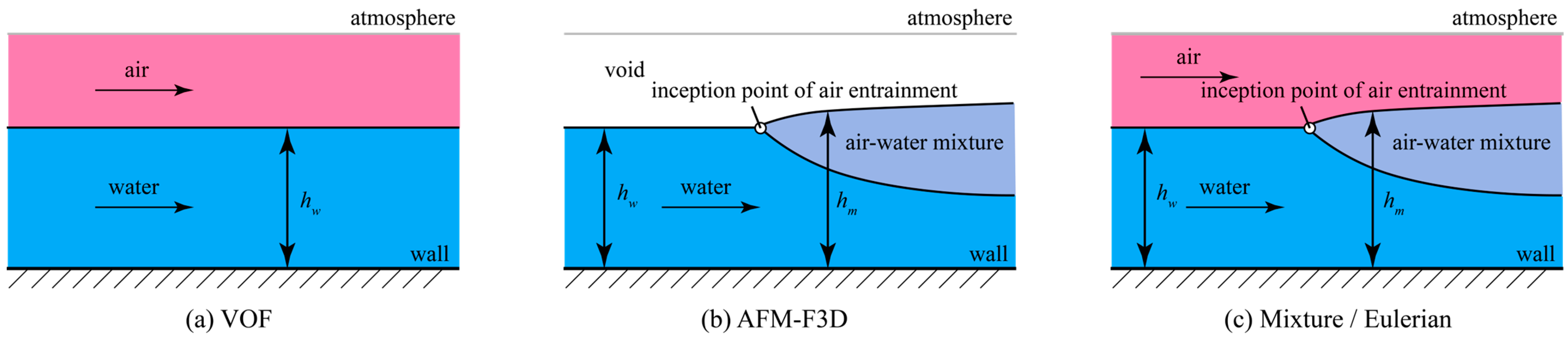
2.1. Comparative Introduction

Generally speaking, the four models mentioned above all belong to the Euler–Euler approach, in which different phases are treated mathematically as continua. Computational grids are introduced to discretize the simulation domain, and the spatial distribution of different phases is dynamically resolved using the volume of fluid (VOF, see [42]) method. The main differences among these four models lie in the specific techniques used to track phase fractions, the treatment of the upper continuous air phase, and the sub-models employed for phase interaction modeling. Figure 1 illustrates the treatment of air–water interfaces and continuous air phases in the four investigated models. It should be emphasized that the following descriptions of the models are based on air–water two-phase flow, though some models can be applied to situations involving more than two fluids.

The term “VOF model” here specifically refers to the VOF multiphase model in Ansys Fluent, rather than the general volume-of-fluid method for phase fraction tracking [42]. This model is primarily used for problems where the location of the large-scale interfaces (i.e., interfaces several times larger than the grid size) is the main concern, whereas it cannot account for phase interpenetration or relative motion between dispersed and continuous phases. Consequently, it is typically used to simulate non-aerated flows in hydraulic engineering. To maintain the sharpness of the air–water interfaces, special methods suppress numerical diffusion, limiting the air–water mixture to 1–2 interface-normal grids.

Both the Mixture and Eulerian models simulate aeration phenomena by allowing the diffusion of large-scale air–water interfaces (i.e., without using special algorithms to keep the interface sharp). Their main difference lies in the number of equations solved. The Mixture model treats the air–water mixture as a mixed fluid with spatially varying density and viscosity and constructs a set of mass and momentum equations for the mixture flow. The Eulerian model, on the other hand, solves a separate set of mass and momentum conservation equations for water and air, respectively.

AFM-F3D utilizes a unique technique called Tru-VOF. This method dynamically detects the large-scale air–water interface (i.e., water surface) and applies dynamic boundary conditions at this interface. As a result, the computational domain is reduced to only the water phase, effectively neglecting the inertia of the gas phase [42,43,44]. For flow with surface aeration, it introduces a source term in the continuity equation to account for the induced flow bulking, treats the mixture of water and entrained air as a pseudo-water phase, and involves additional models to calculate the amount of air that is entrained at each surface cell, as well as its transportation within the fluid domain.

2.2. The VOF Model in Ansys Fluent

The continuity equation of the VOF model is given in the form of the volume-weighted average density ${\rho }_m$ and velocity $U_{mi}$ of the air–water mixture as follows:

$${\displaystyle \frac{𝜕{\rho }_m}{𝜕t}}+{\displaystyle \frac{𝜕}{𝜕x_i}}\left({\rho }_m{U}_{mi}\right)=0$$

(1)

where the subscript m denotes the mixture of two phases, while a and w represent air and water, respectively, in all subsequent references.

Momentum conservation is mathematically expressed as follows:

$${\displaystyle \frac{𝜕\left({\rho }_m{U}_{mi}\right)}{𝜕t}}+{\displaystyle \frac{𝜕}{𝜕x_j}}\left({\rho }_m{U}_{mi}{U}_{mj}\right)=-{\displaystyle \frac{𝜕p}{𝜕x_i}}+{\displaystyle \frac{𝜕}{𝜕x_j}}({\tau }_{ji,m}+{\tau }_{ji,t,m})$$

(2)

where p is pressure, ${\tau }_{ji,m}$ is the viscous forces, ${\tau }_{ji,t,m}$ is the Reynolds stresses calculated using the Boussinesq hypothesis, and the body forces (i.e., gravity) are omitted.

The volume fraction of air and water is dynamically tracked by solving the volume-of-fluid equation as follows:

$${\displaystyle \frac{𝜕{\alpha }_a}{𝜕t}}+{\displaystyle \frac{𝜕}{𝜕x_i}}\left({\alpha }_a{U}_i\right)=0$$

(3)

Based on the research of Bombardelli et al. [45], Morovati et al. [46], and Bayon et al. [47], the RNG k-ε model is more reliable than other alternatives for simulating the flow characteristics of stepped spillways, particularly in consideration of the complex geometries and resulting strong shear effects. Therefore, the RNG k-ε model [48] was employed to account for turbulence contributions to the velocity field. This model considers turbulence effects through transport equations for turbulent kinetic energy k and turbulent dissipation rate ε, which are expressed as follows:

$${\displaystyle \frac{𝜕\left({\rho }_m{k}_m\right)}{𝜕t}}+{\displaystyle \frac{𝜕}{𝜕x_i}}\left({\rho }_m{k}_m{U}_{m,i}\right)={\displaystyle \frac{𝜕}{𝜕x_j}}\left({\rho }_m{D}_k^{eff}{\displaystyle \frac{𝜕k_m}{𝜕x_j}}\right)+{{\rho }_{m}P}_k-{\rho }_m{\epsilon }_m$$

(4)

$${\displaystyle \frac{𝜕\left({\rho }_m{\epsilon }_m\right)}{𝜕t}}+{\displaystyle \frac{𝜕}{𝜕x_i}}\left({\rho }_m{\epsilon }_m{U}_{m,i}\right)={\displaystyle \frac{𝜕}{𝜕x_j}}\left({\rho }_m{D}_{\epsilon }^{eff}{\displaystyle \frac{𝜕{\mathsf{\epsilon }}_m}{𝜕x_j}}\right)+{C_{1\epsilon }{\rho }_{m}P}_k{\displaystyle \frac{{\epsilon }_m}{k_m}}-C_{2\epsilon }^{\ast }{\rho }_m{\displaystyle \frac{{\epsilon }_m^2}{k_m}}$$

(5)

where D_k and D_ε represent the effective diffusivity of k and ε. P_k is the generation of k due to the mean velocity gradients. The model parameter $C_{1\epsilon }$ is 1.42, and $C_{2\epsilon }^{\ast }$ can be calculated from C₂ = 1.68, k, and P_k. More details about the RNG k-ε turbulence model can be found in the user manual of the software [41].

2.3. The Mixture Model in Ansys Fluent

The continuity and momentum equations of the Mixture model closely mirror those of the VOF model. The key distinction lies in the introduction of an additional momentum source term $M_{ip}$, which accounts for the drift motion effect of air and water with regard to the mixture. $M_{ip}$ is calculated as follows:

$$M_{ip}=-{\displaystyle \frac{𝜕}{𝜕x_j}}\left({{\alpha }_a\rho }_a{U}_{dr,a,i}{U}_{dr,a,i}+{{\alpha }_w\rho }_w{U}_{dr,w,i}{U}_{dr,w,i}\right)$$

(6)

where $U_{dr,k}=U_k-U_m$ (k stands for any physical phase, i.e., air or water) is the drift velocity relative to the mixture, which is related to the relative (slip) velocity. The Mixture model assumes local equilibrium between phases over short spatial distances [49], enabling the use of an algebraic relationship for the slip velocity. It is determined as follows:

$${\mathit{U}}_{\mathit{d}\mathit{r},\mathit{p}}={\mathit{U}}_{\mathit{p}\mathit{q}}-{\displaystyle \frac{{\alpha }_p{\rho }_p}{{\rho }_m}}{\mathit{U}}_{\mathit{q}\mathit{p}}$$

(7)

$${\mathit{U}}_{\mathit{p}\mathit{q}}={\displaystyle \frac{{\tau }_p}{f_{drag}}}{\displaystyle \frac{({\rho }_p-{\rho }_m)}{{\rho }_p}}\mathit{a}-{\displaystyle \frac{{\eta }_t}{{\sigma }_t}}({\displaystyle \frac{{\nabla \alpha }_p}{{\alpha }_p}}-{\displaystyle \frac{{\nabla \alpha }_q}{{\alpha }_q}})$$

(8)

where subscripts p and q represent the secondary and primary phases, respectively. ${\tau }_p$ is the particle relaxation time, $f_{drag}$ is the drag function [50], a is the acceleration, and the last term is involved to account for the relative motion induced by turbulent diffusion. In this term, ${\eta }_t$ is the turbulent diffusivity, and ${\sigma }_t$ = 0.75 is the Prandtl/Schmidt number. Considering the significant scale difference between the air bubble/water droplet and the stepped spillway, the inter-phase drag was modeled using the universal drag model [51]. The aforementioned parameters are calculated using the following equations:

$${\tau }_p={\displaystyle \frac{{\rho }_p{d}_p^2}{18{\mu }_q}}$$

(9)

$$f_{drag}={\displaystyle \frac{C_{D}Re}{24}}$$

(10)

$$Re={\displaystyle \frac{{\rho }_q|{\mathit{U}}_{\mathit{q}}-{\mathit{U}}_{\mathit{p}}|d_p}{{\mu }_e}}$$

(11)

$$\mathit{a}=\mathit{g}-\left({\mathit{U}}_{\mathit{m}}·\nabla \right){\mathit{U}}_{\mathit{m}}-{\displaystyle \frac{{𝜕\mathit{U}}_{\mathit{m}}}{𝜕t}}$$

(12)

$${\eta }_t=C_{\mu }{\displaystyle \frac{k^2}{\epsilon }}\left({\displaystyle \frac{{\gamma }_{\gamma }}{1+{\gamma }_{\gamma }}}\right){(1+C_{\beta }{\zeta }_{\gamma }^2)}^{-1/2}$$

(13)

$${\zeta }_{\gamma }={\displaystyle \frac{\left|{\mathit{U}}_{\mathit{p}\mathit{q}}\right|}{\sqrt{2/3k}}}$$

(14)

where $d_p$ is the bubble diameter, ${\mu }_e$ is the effective viscosity of the primary phase accounting for the effects of family of particles in the continuum, $C_D$ is the drag coefficient, Re is the bubble/droplet Reynolds number, and ${\gamma }_{\gamma }$ is the time ratio between the time scale of the energetic turbulent eddies affected by the crossing-trajectories effect and the particle relaxation time. The drag coefficient $C_D$ is defined differently for bubbly and droplet flows and depends mainly on the particle Reynolds number and flow regimes, details of which can be found in [41].

2.4. The Eulerian Model in Ansys Fluent

The Eulerian model constructs separate conservation equations for each phase, adding source terms to account for inter-phase transfers [52]. The mass and momentum equations are:

$${\displaystyle \frac{𝜕\left({\alpha }_k{\rho }_k\right)}{𝜕t}}+{\displaystyle \frac{𝜕}{𝜕x_i}}\left({\alpha }_k{\rho }_k{U}_{ki}\right)=0$$

(15)

$${\displaystyle \frac{𝜕\left({\alpha }_k{\rho }_k{U}_{ki}\right)}{𝜕t}}+{\displaystyle \frac{𝜕}{𝜕x_j}}\left({\alpha }_k{\rho }_k{U}_{ki}{U}_{kj}\right)=-{\alpha }_k{\displaystyle \frac{𝜕p}{𝜕x_i}}+{\displaystyle \frac{𝜕}{𝜕x_j}}\left[{\alpha }_k\left({\tau }_{ji,k}+{\tau }_{ji,t,k}\right)\right]+{\alpha }_k{\rho }_{k}g+M_{i,k}$$

(16)

where the variables are the same as those in Equations (1)–(3), and the inter-phase momentum transfer includes several factors, with only the drag Force $F_{drag}$ and turbulent dispersion force $F_{td}$ considered in this paper. The flow turbulence in the Eulerian model can be considered in several different ways, and the mixture turbulence approach was chosen in this paper, which solves the turbulence transport equation for the air–water mixture using the same equation as shown in Equations (4) and (5).

The inter-phase drag force was also modeled using the universal drag model but with a formulation that differed slightly from the Mixture model:

$$F_{drag}={\displaystyle \frac{{\rho }_p{f}_{drag}}{{6\tau }_p}}{d}_p{A}_i(U_p-U_q)$$

(17)

where $A_i$ is the interfacial area [53], and other variables are identical to those described above.

The model developed by Simonin and Viollet [54] was used to calculate the dispersion force, the equations are as follows:

$$F_{td,q}={-F}_{td,p}=-f_{td,limiting}{C_{TD}K}_{pq}{\displaystyle \frac{D_{t,pq}}{{\sigma }_{pq}}}({\displaystyle \frac{{\nabla \alpha }_p}{{\alpha }_p}}-{\displaystyle \frac{{\nabla \alpha }_q}{{\alpha }_q}})$$

(18)

$$f_{td,limiting}\left({\alpha }_p\right)=\mathrm{m}\mathrm{a}\mathrm{x}(0,\mathrm{m}\mathrm{i}\mathrm{n}(1,{\displaystyle \frac{{\alpha }_{p2}-{\alpha }_p}{{\alpha }_{p2}-{\alpha }_{p1}}}\left)\right)$$

(19)

where $f_{td,limiting}$ is a limiting coffecient, $C_{TD}$ is a user-defined tuning factors that equals 1 by default, $D_{t,pq}$ is the mixture turbulent kinematic viscosity, ${\sigma }_{pq}$ = 0.75 is the dispersion Prandtl number, and ${\alpha }_{p1}$ and ${\alpha }_{p2}$ are the threshold volume fractions of the dispersed phase with default values of 0.3 and 0.7, respectively.

2.5. The Aerated Flow Model in FLOW-3D

The continuity equation of the AFM-F3D model is as follows:

$$V_F{\displaystyle \frac{𝜕{\rho }_m}{𝜕t}}+{\displaystyle \frac{𝜕}{𝜕x_i}}\left({\rho }_m{U}_{mi}{A}_{fi}\right)=S_{\rho }$$

(20)

where $V_F$ is the fractional volume open to flow, $A_{fi}$ is the fractional area of the cell face open to flow, and $S_{\rho }$ is the source term caused by air entrainment.

The surface of the pseudo-water phase is dynamically tracked using the following equation:

$$V_F{\displaystyle \frac{𝜕{\alpha }_w}{𝜕t}}+{\displaystyle \frac{𝜕}{𝜕x_i}}\left(U_{mi}{A}_i{\alpha }_w\right)=S_a$$

(21)

where ${\alpha }_w$ is the water volume fraction and $S_a$ is the fractional air entrainment rate, i.e., the fractional volume of air entrained into the cell per second.

Once the pseudo-water surface is detected and the fluid domain is determined, the momentum and turbulent transport equations (see Equations (2), (4), and (5)) are solved for the mixture of water and entrained air.

The air entrainment model in FLOW-3D assumes that surface aeration takes place when the destabilizing force $P_t$, which is linearly related to the turbulent kinetic energy, overcomes the stabilizing force P_d, which is a function of gravity and surface tension [55]. Air with a certain volume of $\delta V$ will be entrained into the water according to the following:

$$\delta V=\left\{\begin{array}{c}{k}_{air}{A}_s\left[{\displaystyle \frac{2\left(P_t{-P}_d\right)}{{\rho }_w}}\right] if P_t{>P}_d\\ 0 if P_t{<P}_d\end{array}\right.$$

(22)

$$L_T={\displaystyle \frac{{CNU}^{3/4}{k}^{3/2}}{\mathsf{\epsilon }}}$$

(23)

$$P_t={\rho }_m{k}_T$$

(24)

$$P_d={\rho }_m{g}_n{L}_T+{\displaystyle \frac{\sigma }{L_T}}$$

(25)

where $L_T$ represents the turbulence length scale, CNU = 0.09, $g_n$ is the component of gravity normal to the water surface, $\sigma$ is the coefficient of surface tension, $\delta V$ is the volume of air entrained per unit time, $k_{air}$ is a coefficient, and $A_s$ is the surface area.

To simulate the transportation of the entrained air bubbles within the fluid domain, a so-called drift-flux model [56,57] is adopted in FLOW-3D, by which the buoyancy, phase drag, and the bubble–bubble interaction effects are considered. In this model, the relative velocity between the dispersed and the continuous phases is considered steady, and thus the air transport equation yields the following:

$$\left({\displaystyle \frac{1}{{\rho }_w}}-{\displaystyle \frac{1}{{\rho }_a}}\right)\nabla P=\left({\displaystyle \frac{{\alpha }_w{\rho }_w+{\alpha }_a{\rho }_a}{{\alpha }_w{\alpha }_a{\rho }_w{\rho }_a}}\right){Ku}_r$$

(26)

where ${\alpha }_w$ is the volume fraction of water, K is the drag coefficient, and $u_r$ represents the relative velocity. K can be calculated from the single-particle drag coefficient $K_P$:

$$K_p={\displaystyle \frac{1}{2}}{A}_p{\rho }_a\left(C_d{U}_r+{\displaystyle \frac{12{\mu }_a}{{\rho }_a{R}_p}}\right)$$

(27)

$$K={\displaystyle \frac{(1-f)}{V_P}}{K}_P$$

(28)

where $A_p$ is the cross-sectional area of the air bubble, $U_r$ is the magnitude of $u_r$, $C_d$ is a user-defined drag coefficient [44], ${\mu }_a$ is the dynamic viscosity of air, $V_p$ is the volume of a single bubble, and $R_p$ denotes the bubble radius, which is controlled by the critical Weber and capillary numbers to account for the bubble breakup and coalescence. More details of the AFM-F3D can be found in the user manual [58].

3. Test Case and Simulation Setup

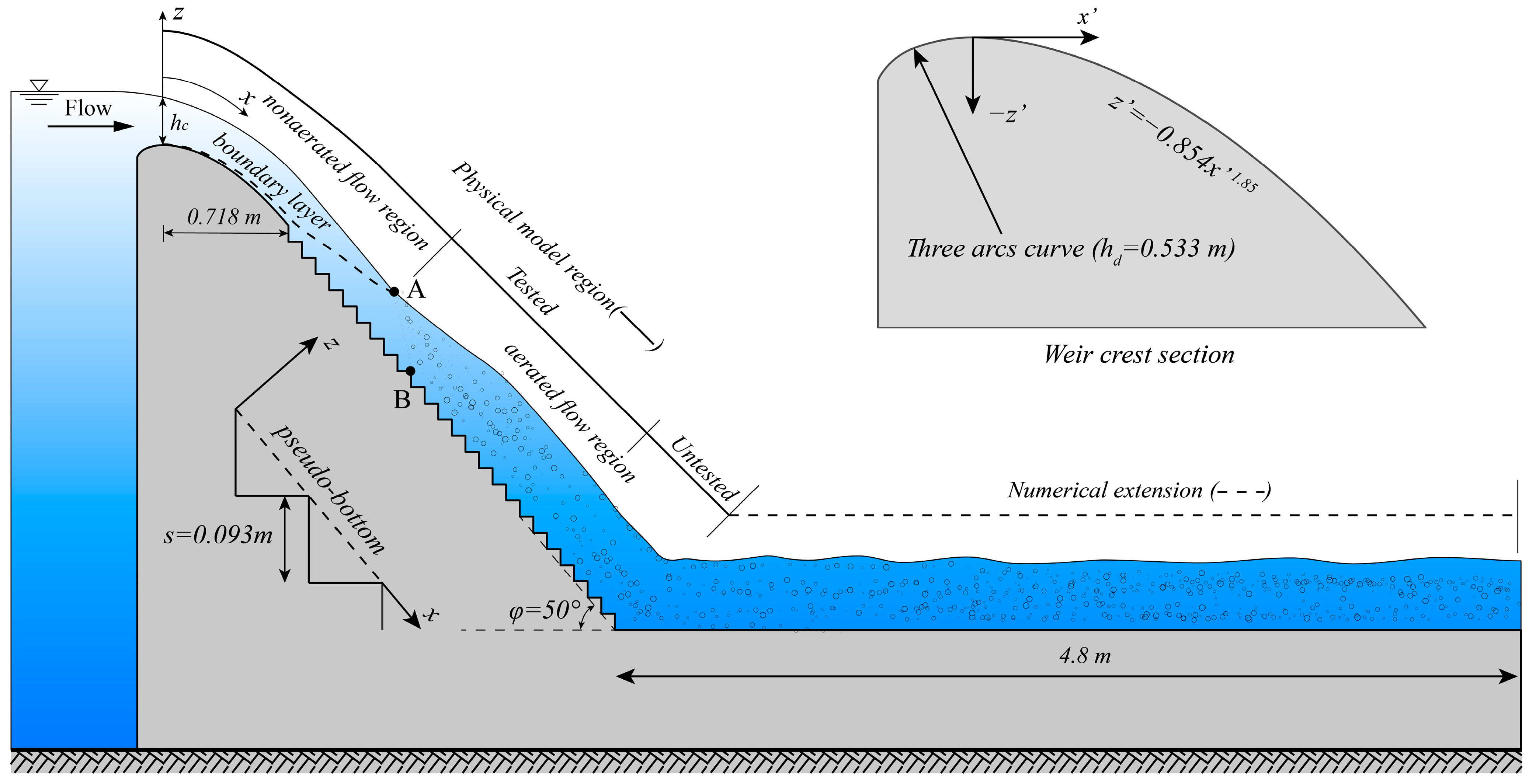
3.1. Test Case

The stepped spillway physical model of Pfister and Hager [59] was selected for the comparative model evaluation in this paper. The stepped chute was 0.5 m wide and 3.4 m long, comprising 25 uniform steps, each 0.093 m high and 0.078 m wide (Figure 2). It featured a standard-crest profile with a design head of 0.533 m and a downstream inclination of 50°. The chute was extended horizontally by 4.8 m downstream of the last step in the simulation to obtain fully developed, uniform flow at the outlet boundary (Figure 2). Our study focused on the specific condition with a unit discharge of 0.215 m²/s, corresponding to a weir crest flow depth of 0.167 m. Under this condition, the physical model exhibited an inception point of air entrainment at x = 1.53 m, i.e., approximately at the 6th step.

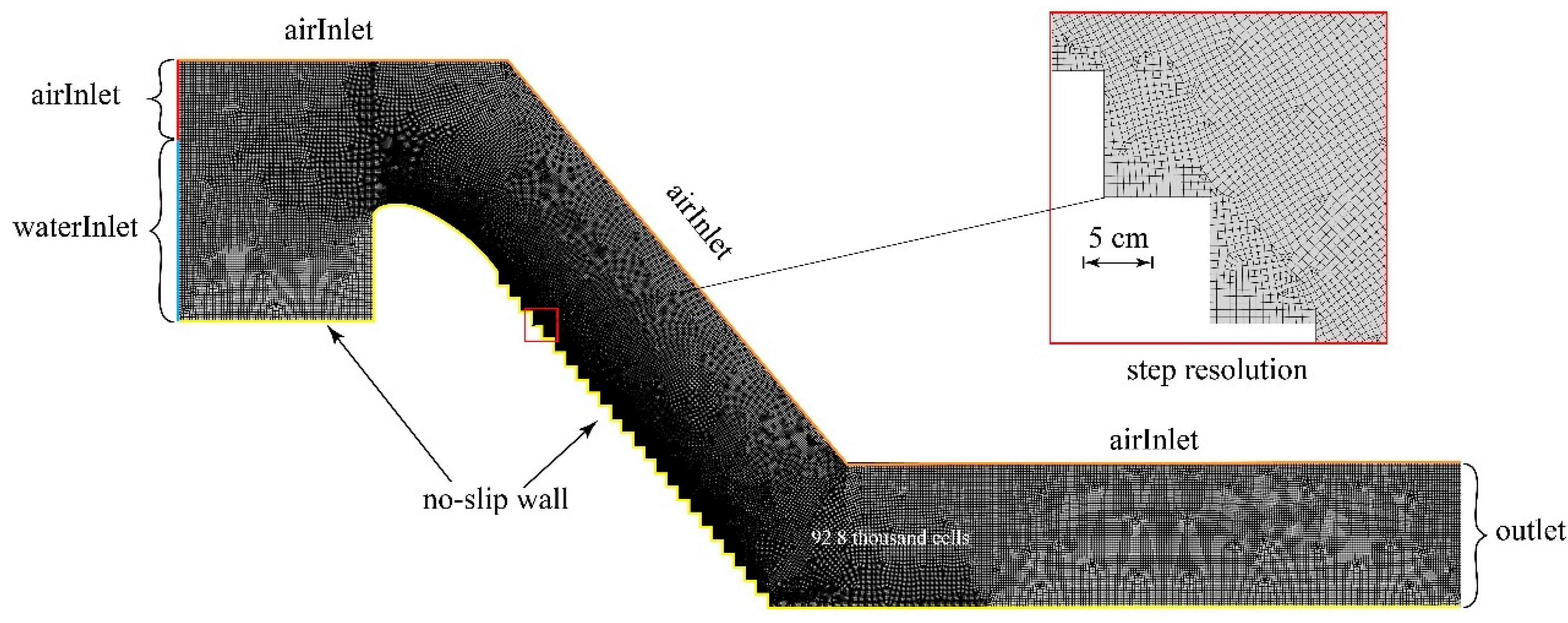
3.2. Simulation Setup in Ansys Fluent

In Ansys Fluent, the computational grids were generated using Ansys ICEM, and a mesh of 92,800 cells was finally used based on the grid convergence study (see Appendix A). The mesh features an average spatial resolution of approximately 5 mm near the step surface, as shown in Figure 3. The pressure inlet boundary condition (BC) is applied at both the top and air inlet, with total pressure P₀ = 0 Pa, turbulent kinetic energy k = 1 × 10⁻³ m²/s², and turbulent dissipation rate ε = 1 × 10⁻³ m²/s³. The water inlet was set as a pressure inlet with hydrostatic pressure specified based on a water level of 0.227 m. The turbulence parameters are specified as turbulence intensity I_t = 5% and turbulence length scale L_t = 0.072 m. The outlet is set as a pressure outlet with a total pressure of P₀ = 0 Pa, and the turbulence parameters for the backflow air are k = 1 × 10⁻³ m²/s² and ε = 1 × 10⁻³ m²/s³. The bottom is set as a no-slip smooth wall. The air bubble diameter is set to a constant value of 1 mm based on the literature [37]. The numerical schemes of the spatial and temporal discretization adopted for the tested models are listed in

Table 1. The model’s implemented numerical schemes.

Pressure–Velocity Coupling		PISO
Gradient		Green-Gauss Cell Based
Pressure		PRESTO!
Momentum		Second-order upwind
Volume fraction	VOF	Geo-reconstruct
	Mixture	QUICK
	Eulerian	QUICK
Turbulence quantities (k and ε)		First-order upwind

.

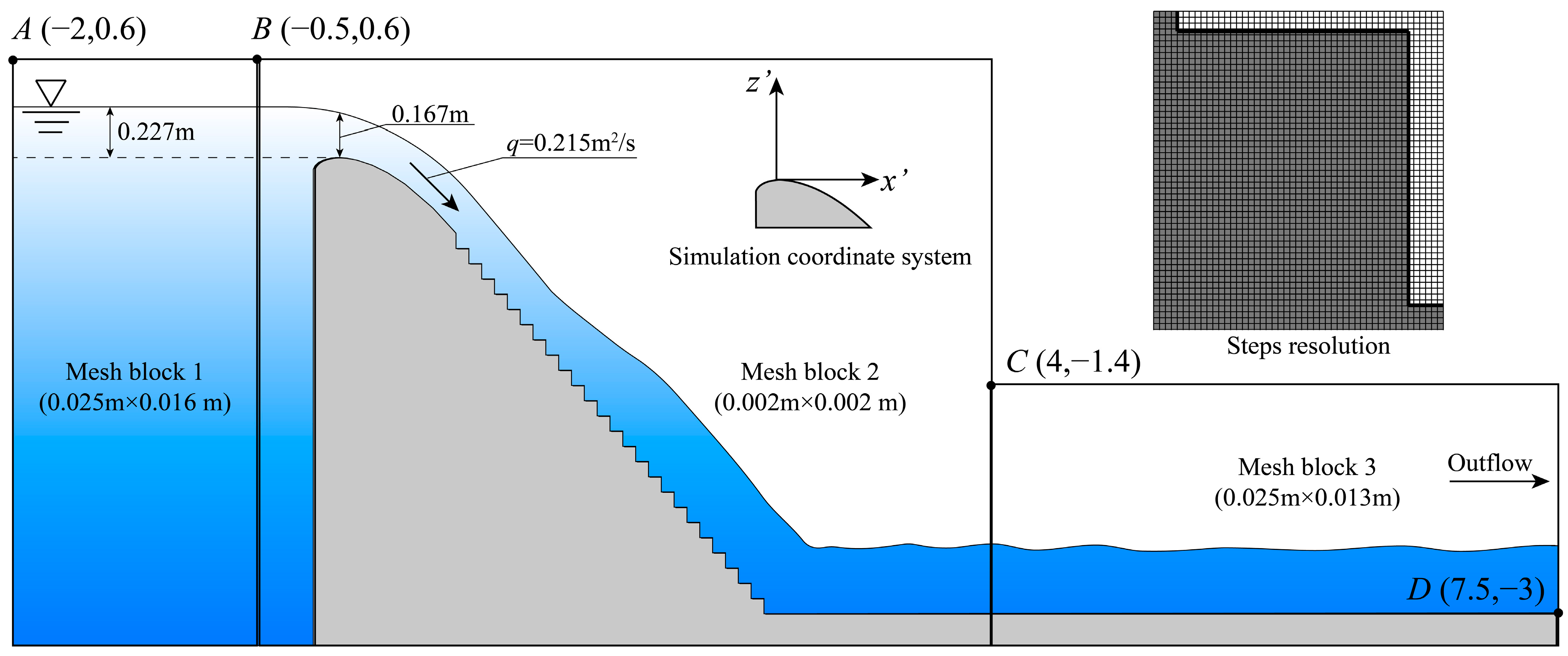
3.3. Simulation Setup in FLOW-3D

In FLOW-3D, three linked mesh blocks were used to resolve the spillway structure and fluid domain using the FAVOR^® technique. The location of the mesh blocks is shown in Figure 4, and mesh block 2 covers the entire physical model region. The cell sizes of the mesh blocks were 0.025 × 0.016 m, 0.002 × 0.002 m, and 0.025 × 0.013 m, respectively. These cell sizes were determined based on a previous simulation of the identical spillway case using FLOW-3D [35]. The inlet was set as hydrostatic pressure calculated with a weir head of 0.227 m, while the downstream boundary was defined as outflow. The top and bottom boundaries were set as atmosphere and no-slip wall, respectively.

There are several user-defined parameters for air entrainment modeling. In this study, bubble diameters were dynamically computed with an initial drop diameter of 1 mm. The critical Weber and capillary numbers were kept at their default values of 1.6 and 1, respectively. For the drag force and bubble interaction, default values of 0.5 and 1 were used for the drag coefficient and Richardson–Zaki coefficient multiplier, respectively. The minimum and maximum volume fractions of water were 0.1 and 1, respectively, as the software suggested. The density and viscosity of air were set to 1.225 kg/m³ and 1.7 × 10⁻⁵ kg/m/s. Lastly, the critical air volume fraction that controls the transition of air from dispersed to continuous was defined as 1, and gas escape was allowed.

4. Simulation Results

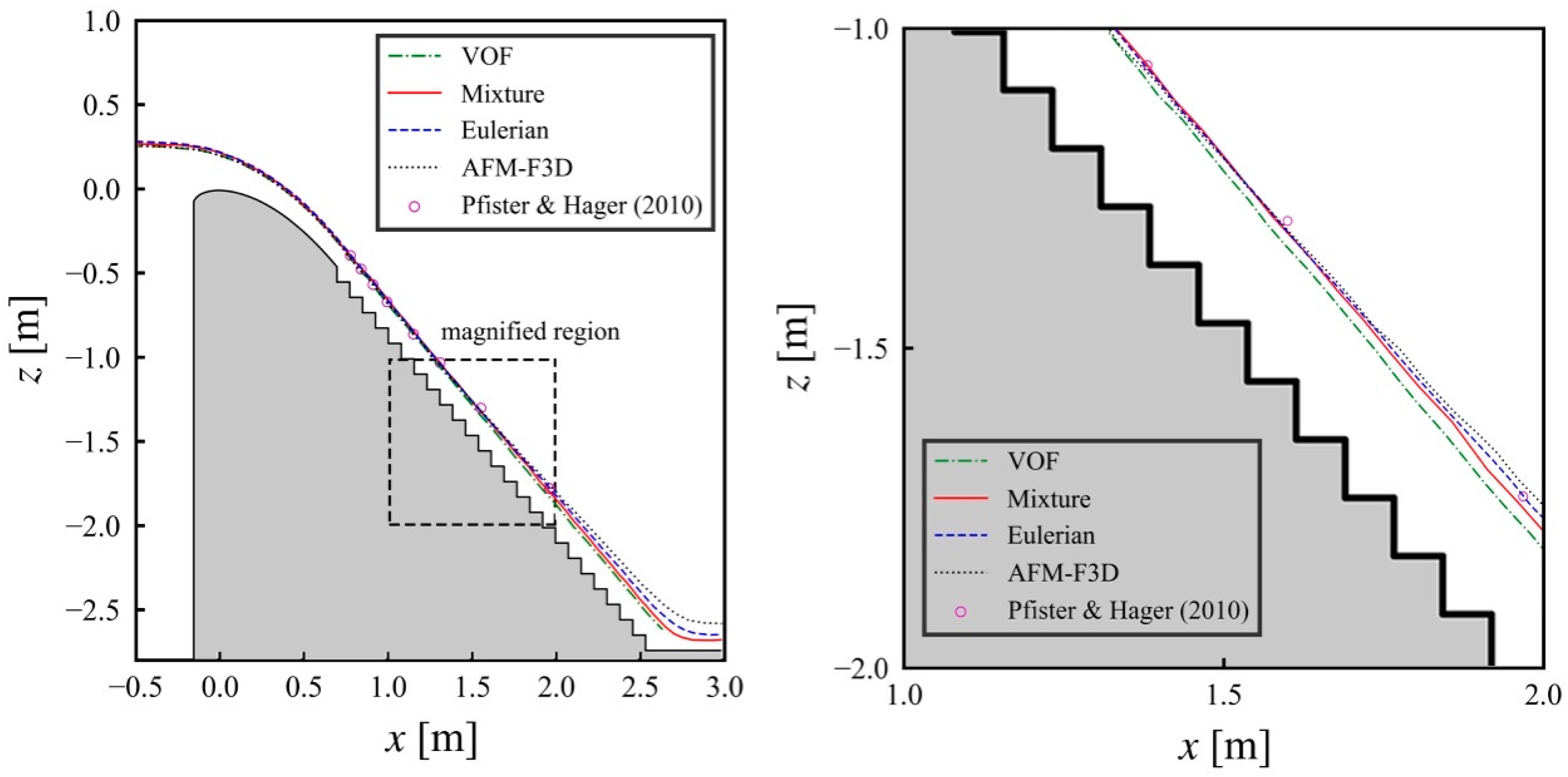
4.1. Surface Profile

Figure 5 compares the measured and simulated aerated surface profiles using four different models. All four tested models show excellent agreement with measurements in the non-aerated region (i.e., upstream of approximately the 6~7th step). However, in the aerated region, the VOF model significantly underestimates the aerated water depth due to its inability to account for air entrainment at the water surface. In contrast, the aerated surface obtained with the other three models generally aligned well with the experimental data, with only minor differences. AFM-F3D yields the deepest aerated water surface profile, followed by the Eulerian model, with the Mixture model producing the shallowest profile. Due to the limited number of measurement points in the aerated region, it is challenging to definitively evaluate the accuracy of these three models.

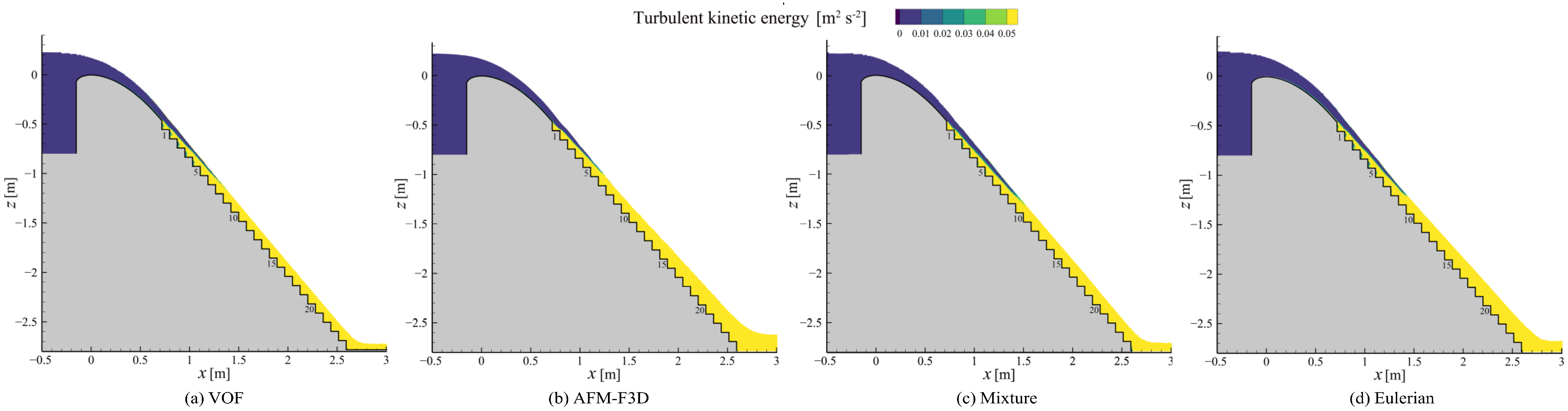
4.2. Turbulence Development and Air Entrainment Onset

Figure 6 illustrates the distribution of TKE in the non-aerated regions as calculated by the four different models. It has been discovered by Bombardelli et al. [44] and Meireles et al. [60] that the air entrainment model in FLOW-3D predicted the inception point of air entrainment that overlapped well with experimental observations. According to the literature [35], which simulated the identical case of our current stepped spillway case with FLOW-3D, a minimum TKE value of k ≈ 0.05 m²/s² is required for self-aeration to occur in the investigated case. Consequently, the colormap range of Figure 6 is set to 0–0.05 m²/s² to evaluate each model’s ability to capture the inception point. It is evident that the VOF and AFM-F3D models effectively capture the inception point of air entrainment. In contrast, the Mixture and Eulerian models predict an inception point slightly downstream, around the 9~10th steps, indicating a slower turbulent development. A detailed quantitative analysis of the turbulent development is presented in Section 4.5.

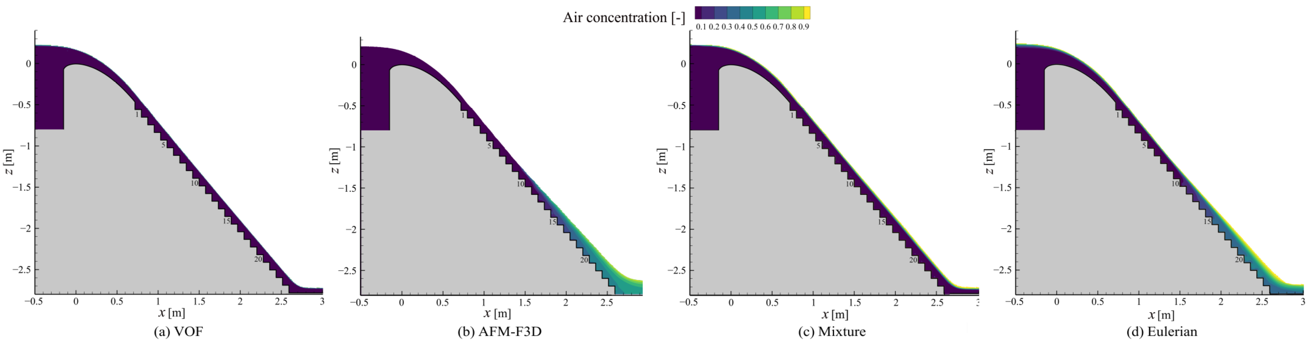
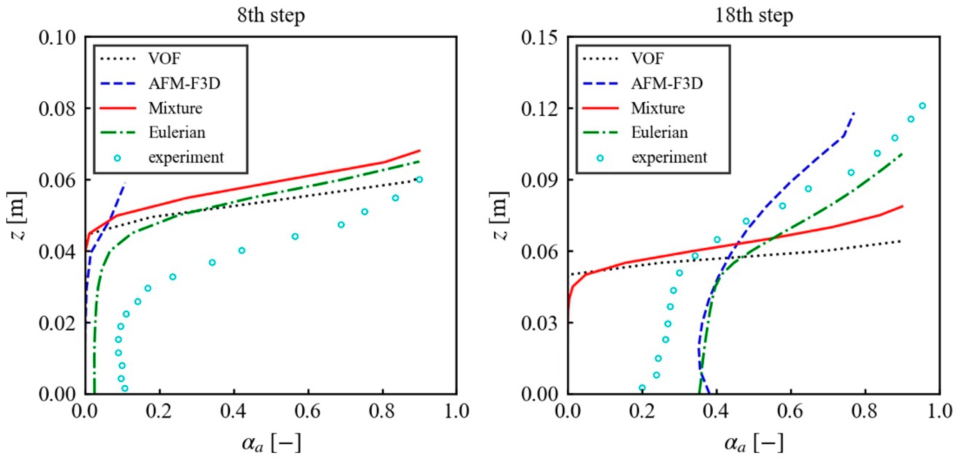
4.3. Air Concentration

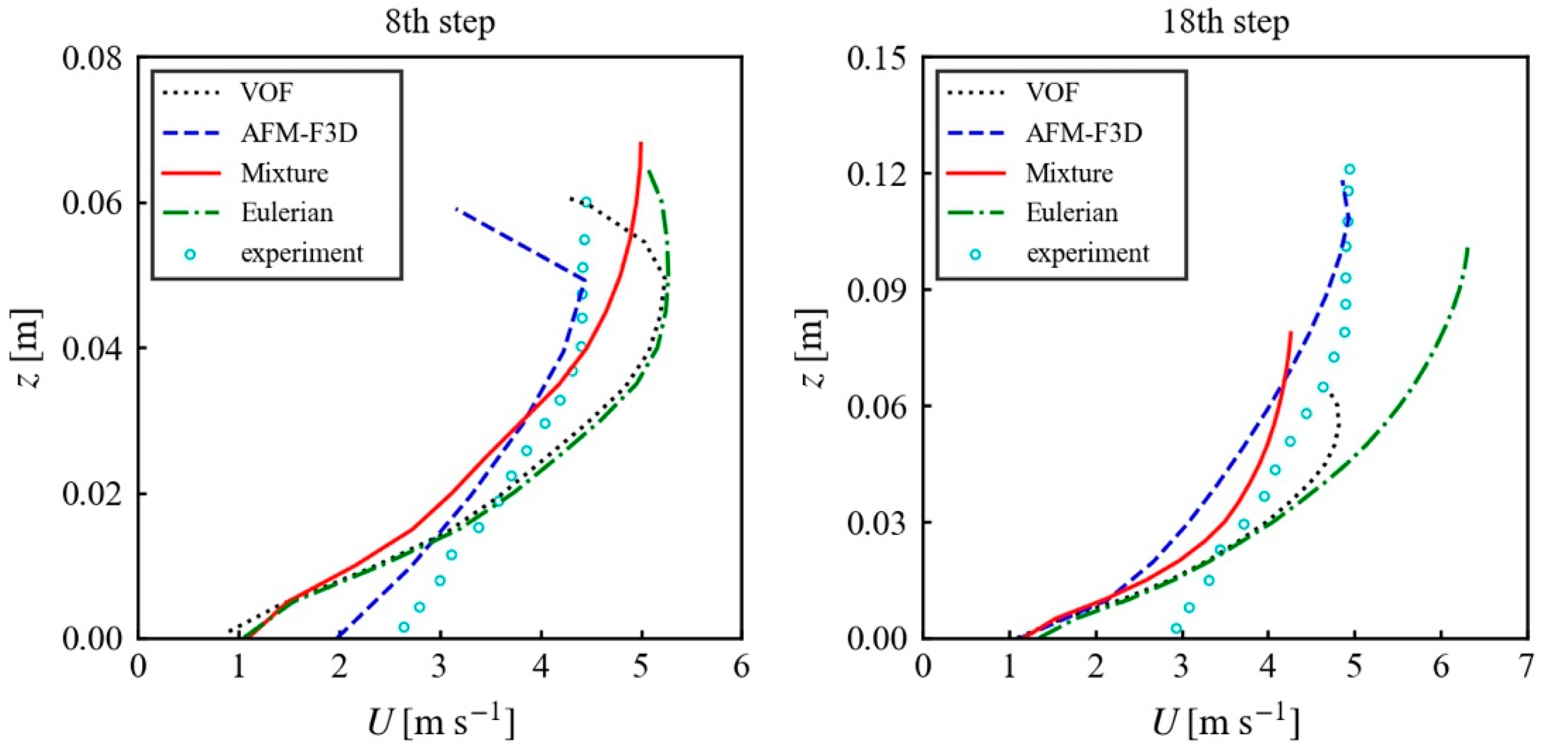
Figure 7 presents the air concentration distribution calculated by four different models. AFM-F3D and the VOF model yield a very sharp interface in the non-aerated region, while the Mixture and Eulerian models produce a slightly diffusive interface, which is evidently due to the different schemes they adopted to solve the volume of fluid equations. This indicates that the geometric schemes of Donor–Accepter and Geo-reconstruct are more effective at maintaining the sharpness of the interface compared to the QUICK scheme. Moreover, notable air entrainment and downward transport are only observable with AFM-F3D and the Eulerian model, indicating that the VOF and Mixture models are not suitable for aerated flows.

To quantitatively compare the four tested models’ ability to reproduce the air concentration distributions, simulated air concentration distributions perpendicular to the pseudo-bottom at the 8th and 18th steps are shown in Figure 8, in comparison with the measured data. At the 8th step, near the inception point, all four models underestimate air entrainment and subsequent downward transport. Specifically, AFM-F3D produces the weakest air entrainment, with a surface air concentration as low as roughly 0.1. In contrast, the other three models capture the rapid air–water transition at the interfacial regions featuring air concentration ranging from 0.1~0.9. Notable differences exist between these three models. The Eulerian model transports entrained air to the step surface, with a bottom air concentration of approximately 0.02. The VOF and Mixture models, however, only track entrained air slightly beneath the aerated water surface, roughly at 0.04 m < z < 0.06 m.

At the 18th step, where aeration is significantly developed, the VOF model still fails to reproduce the surface aeration, maintaining a sharp interface. Similarly, the Mixture model returns a slightly thicker interface, with an aeration penetration depth of about 0.03 m. Conversely, AFM-F3D and the Eulerian models both produce S-shaped air concentration profiles, resembling the measured profile. Notably, the lower part (i.e., below z ≈ 0.06 m) of these two simulated profiles overlaps well with each other and runs almost parallel to the measurement. However, they exhibit a bottom air concentration of approximately 0.4—nearly double the experimental value of 0.2. In the upper half-region, while the Eulerian model’s profile generally remains parallel to the experimental profile, the air concentration calculated by AFM-F3D increases slowly with bottom distance compared to the Eulerian model and the experiment, reaching a surface air concentration of only 0.7. The above differences are clearly related to the turbulent intensity dominating the air transport process, which is illustrated in detail hereafter.

4.4. Velocity

Figure 9 compares the measured and simulated velocity distributions perpendicular to the pseudo-bottom at the 8th and 18th steps, as calculated by the four different models. All four models produce velocity distribution profiles generally similar to the measurements. However, the simulated pseudo-bottom velocities are significantly lower than the experimental values, and the simulated velocity gradients are generally steeper. This can be ascribed to the drag reduction effect [61,62] of entrained air, which is not considered in the numerical models. Overall, discrepancies are more pronounced at the 18th step (significantly aerated) compared to the 8th step (slightly aerated). Among the four tested models, AFM-F3D’s velocity profile matches the measurement best, and the Eulerian model yields a higher velocity gradient and surface velocity roughly 25% larger than the measurement. Analysis of the velocities calculated by the VOF and Mixture models is omitted due to their inability to reproduce the air entrainment phenomenon.

4.5. Turbulent Kinetic Energy

The TKE distributions calculated by four models are presented in Figure 10. The Mixture model produces TKE values significantly lower than the other three models, which explains its inability to produce air entrainment and transport phenomena. In comparison, the differences between the other three models are minimal. The VOF model and AFM-F3D return almost identical TKE distributions, while the Eulerian model yields an additional low TKE region in the upper part of the aerated region.

The TKE distributions perpendicular to the pseudo-bottom at the 8th and 18th steps, calculated by the four models, are presented in Figure 11. It can be observed that these four models produce TKE profiles with similar shapes: TKE increases near the pseudo-bottom and then decreases throughout the flow. However, the TKE values returned by the four models differ significantly. AFM-F3D yields the highest TKE values, followed by the VOF and Eulerian models, with slight differences between them, and the Mixture model predicts TKE values significantly lower than the others. At the 18th step, the TKE values calculated using AFM-F3D decrease almost linearly from the pseudo-bottom to the aerated surface. Interestingly, the VOF model produces a slight enhancement of TKE at the water surface—a feature absent in the other models.

5. Conclusions

In the current paper, four multiphase models, namely the VOF, Mixture, and Eulerian model in Ansys Fluent and the aerated flow model in FLOW-3D (AFM-F3D), are comparatively introduced for the first time. On this basis, these models are tested for the aerated flow over stepped spillways. The simulation results, including water surface profiles, inception points of aeration, air concentrations, velocities, and turbulent kinetic energies, from these models are compared with each other and with available experimental data. A systematic analysis of the performance of these models yields the following findings:

(1)

All four tested models can generally reproduce the development of the turbulent boundary layer and air entrainment onset in the non-aerated region.

(2)

The VOF model is unable to reproduce the self-aeration phenomenon due to its intrinsic feature of sharpening the interface and not allowing phase interpenetration. The Mixture model significantly underestimates the turbulent kinetic energy within the water phase and thus fails to reproduce the self-aeration and downward air transport phenomena as well. Therefore, the VOF and Mixture models are both not recommended for simulating the aerated flow on stepped spillways.

(3)

Both AFM-F3D and the Eulerian model incorporate mechanisms that account for the main physical effects in aerated flows, and their calculated aerated water surface profiles are generally reliable. However, some discrepancies remain between the calculated air concentrations and velocities from these two models and the measurements. The Eulerian model performs more accurately in terms of air concentration, while AFM-F3D exhibits a slight advantage in velocity distribution calculations. Overall, the Eulerian model is recommended for simulating aerated stepped spillway flows due to its more reasonable physical basis, wider popularity, advantages in resolving spillway geometry and potential for accuracy improvement through parameter tuning.

However, the present study has some limitations. The discretization scheme of the volume-of-fluid equation plays a crucial role in the air concentration results, which is beyond the scope of this study. TKE data were unavailable from the physical model, which would have allowed for deeper analysis of the differences in air concentration and velocity between the experimental and numerical data. Furthermore, sidewall effects may exist in the experiment but were not considered in the current two-dimensional simulation due to computational efficiency constraints.

Nonetheless, the findings from the study are encouraging for the use of advanced numerical modeling techniques in investigating the two-phase characteristics of stepped spillways, especially those with complex geometry or large unit discharges, which have not been adequately explored. Moreover, our findings could offer valuable insights for selecting multiphase models based on different engineering focuses.

References

1. Matos, J.; Meireles, I. Hydraulics of stepped weirs and dam spillways: Engineering challenges, labyrinths of research. In Proceedings of the 5th IAHR International Symposium on Hydraulic Structures, Brisbane, Australia, 25–27 June 2014. [Google Scholar]
2. Baylar, A.; Emiroglu, M.E.; Bagatur, T. An experimental investigation of aeration performance in stepped spillways. Water Environ. J. 2006, 20, 35–42. [Google Scholar] [CrossRef]
3. Felder, S.; Chanson, H. Simple design criterion for residual energy on embankment dam stepped spillways. J. Hydraul. Eng. 2016, 142, 04015062. [Google Scholar] [CrossRef]
4. Luo, S.K.; Li, L.X.; Ru, Y.S. Numerical simulation on stepped spillway in discharge tunnel of Buxi power station. J. Hydroelectr. Eng. 2010, 29, 50–56. (In Chinese) [Google Scholar]
5. Chen, L.Q.; Wang, J.X.; Chen, Y.T. Numerical simulation of stepped energy dissipation in high velocity emptying tunnel. Eng. J. Wuhan Univ. 2014, 47, 28–33. (In Chinese) [Google Scholar]
6. Chanson, H. Prediction of the transition nappe/skimming flow on a stepped channel. J. Hydraul. Res. 1996, 34, 421–429. [Google Scholar] [CrossRef]
7. Chanson, H.; Toombes, L. Hydraulics of stepped chutes: The transition flow. J. Hydraul. Res. 2004, 42, 43–54. [Google Scholar] [CrossRef]
8. Sánchez-Juny, M.; Bladé, E.; Dolz, J. Analysis of pressures on a stepped spillway. J. Hydraul. Res. 2008, 46, 410–414. [Google Scholar] [CrossRef]
9. Sánchez-Juny, M.; Bladé, E.; Dolz, J. Pressures on a stepped spillway. J. Hydraul. Res. 2007, 45, 505–511. [Google Scholar] [CrossRef]
10. Xu, W.L.; Luo, S.J.; Zheng, Q.W. Experimental study on pressure and aeration characteristics in stepped chute flows. Sci. China Technol. Sci. 2015, 58, 720–726. [Google Scholar] [CrossRef]
11. Xie, X.Z.; Li, S.Q.; Li, G.F. Development of flaring gate piers in China II. Hongshui River 1995, 15, 24–30. (In Chinese) [Google Scholar]
12. Boes, R.M. Guideline on the Design and Hydraulic Characteristics of Stepped Spillways; Commission Internationale des Grands Barrages: Kyoto, Japan, 2012. [Google Scholar]
13. Pfister, M.; Hager, W.H.; Minor, H.E. Stepped chutes: Pre-aeration and spray reduction. Int. J. Multiph. Flow 2006, 32, 269–284. [Google Scholar] [CrossRef]
14. Pfister, M.; Hager, W.H.; Minor, H.E. Bottom aeration of stepped spillways. J. Hydraul. Eng. 2006, 132, 850–853. [Google Scholar] [CrossRef]
15. Boes, R.M.; Hager, W.H. Two-phase flow characteristics of stepped spillways. J. Hydraul. Eng. 2003, 129, 661–670. [Google Scholar] [CrossRef]
16. Boes, R.M.; Hager, W.H. Hydraulic design of stepped spillways. J. Hydraul. Eng. 2003, 129, 671–679. [Google Scholar] [CrossRef]
17. Chanson, H. Hydraulics of skimming flows over stepped channels and spillways. J. Hydraul. Eng. 1994, 32, 445–460. [Google Scholar] [CrossRef]
18. Chamani, M.R.; Rajaratnam, N. Characteristics of skimming flow over stepped spillways. J. Hydraul. Eng. 1999, 125, 361–368. [Google Scholar] [CrossRef]
19. Takahashi, M.; Ohtsu, I. Aerated flow characteristics of skimming flow over stepped chutes. J. Hydraul. Eng. 2012, 50, 427–434. [Google Scholar] [CrossRef]
20. Dong, Z.S.; Wang, J.X.; Vetsch, D.F.; Boes, R.M. Numerical simulation of air–water two-phase flow on stepped spillways behind X-shaped flaring gate piers under very high unit discharge. Water 2019, 11, 1956. [Google Scholar] [CrossRef]
21. Hu, Y.H.; Wu, C.; Lu, H.; Zhang, T.; Mo, Z.Y. Study on hydraulic structure of flaring gate piers locating at the upstream of stepped spillway. J. Hydroelectr. Eng. 2006, 25, 37–41. (In Chinese) [Google Scholar]
22. Liang, Z.X.; Yin, J.B.; Zheng, Z.; Lu, H. Aeration of skimming flow on stepped spillway combined with flaring gate piers. J. Hydraul. Eng. 2009, 5, 564–568. (In Chinese) [Google Scholar]
23. Dong, Z.S. Numerical Simulation Study on Destruction Mechanism of the Step Behind the X-Shaped Flairing Gate Piers. Master Thesis, Wuhan University, Wuhan, China, 2017. (In Chinese). [Google Scholar]
24. Chanson, H.; Gonzalez, C.A. Physical modelling and scale effects of air-water flows on stepped spillways. Zhejiang Univ. Sci. 2005, 6, 243–250. [Google Scholar] [CrossRef]
25. Felder, S.; Chanson, H. Turbulence, dynamic similarity and scale effects in high-velocity free-surface flows above a stepped chute. Exp. Fluids 2009, 47, 1–18. [Google Scholar] [CrossRef]
26. Felder, S.; Chanson, H. Scale effects in microscopic air-water flow properties in high-velocity free-surface flows. Exp. Therm. Fluid Sci. 2017, 83, 19–36. [Google Scholar] [CrossRef]
27. Heller, V. Scale effects in physical hydraulic engineering models. J. Hydraul. Res. 2011, 49, 293–306. [Google Scholar] [CrossRef]
28. Pfister, M.; Chanson, H. Discussion of scale effects in physical hydraulic engineering models By Valentin Heller. J. Hydraul. Res. 2012, 50, 244–246. [Google Scholar] [CrossRef]
29. Jesudhas, V.; Balachandar, R.; Bolisetti, T. Numerical study of a symmetric submerged spatial hydraulic jump. J. Hydraul. Res. 2020, 58, 335–349. [Google Scholar] [CrossRef]
30. Witt, A.; Gulliver, J.S.; Shen, L. Numerical investigation of vorticity and bubble clustering in an air entraining hydraulic jump. Comput. Fluids 2018, 172, 162–180. [Google Scholar] [CrossRef]
31. Biswas, T.R.; Dey, S.; Sen, D. Undular hydraulic jumps: Critical analysis of 2D RANS-VOF simulations. J. Hydraul. Eng. 2021, 147, 06021017. [Google Scholar] [CrossRef]
32. Toro, J.P.; Bombardelli, F.A.; Paik, J.; Meireles, I.C.; Amador, A. Characterization of turbulence statistics on the non-aerated skimming flow over stepped spillways: A numerical study. Environ. Fluid Mech. 2016, 16, 1195–1221. [Google Scholar] [CrossRef]
33. Chen, J.G.; Zhang, J.M.; Xu, W.L.; Wang, Y.R. Numerical simulation of the energy dissipation characteristics in stilling basin of multi-horizontal submerged jets. J. Hydrodyn. 2010, 22, 732–741. [Google Scholar] [CrossRef]
34. Eghbalzadeha, A.; Javan, M. Comparison of mixture and VOF models for numerical simulation of air–entrainment in skimming flow over stepped spillways. J. Procedia Eng. 2012, 28, 657–660. [Google Scholar] [CrossRef]
35. Dong, Z.S.; Wang, J.X.; Vetsch, D.F.; Boes, R.M.; Tan, G.M. Numerical simulation of air entrainment on stepped spillway. In Proceedings of the 38th IAHR World Congress, Panama City, Panama, 1–6 September 2019. [Google Scholar]
36. Teng, P.H.; Yang, J.; Pfister, M. Studies of two-phase flow at a chute aerator with experiments and CFD modelling. Model. Simul. Eng. 2016, 2016, 4729128. [Google Scholar] [CrossRef]
37. Yang, J.; Teng, P.H.; Zhang, H.W. Experiments and CFD modeling of high-velocity two-phase flows in a large chute aerator facility. Eng. Appl. Comput. Fluid Mech. 2019, 13, 48–66. [Google Scholar] [CrossRef]
38. Ma, J.S.; Oberai, A.A.; Lahey, R.T.; Drew, D.A. Modeling air entrainment and transport in a hydraulic jump using two-fluid RANS and DES turbulence models. Heat Mass Transf. 2011, 47, 911–919. [Google Scholar] [CrossRef]
39. Zhang, J.M.; Chen, J.G.; Xu, W.L.; Wang, Y.R.; Li, G.J. Three-dimensional numerical simulation of aerated flows downstream sudden fall aerator expansion-in a tunnel. J. Hydrodyn. 2011, 23, 71–80. [Google Scholar] [CrossRef]
40. Mendes, L.S.; Lara, J.L.; Viseu, M.T. Do the Volume-of-Fluid and the Two-Phase Euler compete for modeling a spillway aerator? Water 2021, 13, 3092. [Google Scholar] [CrossRef]
41. ANSYS. ANSYS Fluent Theory Guide; ANSYS Inc.: Canonsburg, PA, USA, 2018. [Google Scholar]
42. Hirt, C.W.; Nichols, B.D. Volume of fluid (VOF) method for the dynamics of free boundaries. J. Comput. Phys. 1981, 39, 201–225. [Google Scholar] [CrossRef]
43. Nichols, B.D.; Hirt, C.W. Improved free surface boundary conditions for numerical incompressible-flow calculations. J. Comput. Phys. 1971, 8, 434–448. [Google Scholar] [CrossRef]
44. Richardson, J.F.; Zaki, W.N. Sedimentation and fluidisation: Part 1. Trans. IChemE 1954, 32, 35–53. [Google Scholar] [CrossRef]
45. Bombardelli, F.A.; Meireles, I.; Matos, J. Laboratory measurements and multi-block numerical simulations of the mean flow and turbulence in the non-aerated skimming flow region of steep stepped spillways. Environ. Fluid Mech. 2011, 11, 263–288. [Google Scholar] [CrossRef]
46. Morovati, K.; Homer, C.; Tian, F.; Hu, H. Opening configuration design effects on pooled stepped chutes. J. Hydraul. Eng. 2021, 147, 06021011. [Google Scholar] [CrossRef]
47. Bayon, A.; Toro, J.P.; Bombardelli, F.A.; Matos, J.; López-Jiménez, P.A. Influence of VOF technique, turbulence model and discretization scheme on the numerical simulation of the non-aerated, skimming flow in stepped spillways. J. Hydro-Environ. Res. 2018, 19, 137–149. [Google Scholar] [CrossRef]
48. Yakhot, S.; Orszag, A. Renormalization group analysis of turbulence. I. Basic theory. J. Sci. Comput. 1986, 1, 3–51. [Google Scholar] [CrossRef]
49. Manninen, M.; Kallio, S. On the Mixture Model for Multiphase Flow; VTT Publications 288; Technical Research Centre of Finland: Espoo, Finland, 1996. [Google Scholar]
50. Ishii, M.; Zuber, N. Drag coefficient and relative velocity in bubbly, droplet or particulate flows. AIChE J. 1979, 25, 843–855. [Google Scholar] [CrossRef]
51. Kolev, N.I. Multiphase Flow Dynamics 2: Thermal and Mechanical Interactions, 2nd ed.; Springer: Berlin, Germany, 2005. [Google Scholar]
52. Ishii, M.; Hibiki, T. Thermo-Fluid Dynamics of Two-Phase Flow; Springer Science & Business Media: Berlin/Heidelberg, Germany, 2010. [Google Scholar]
53. Ishii, M.; Kim, S.; Uhle, J. Interfacial area transport equation: Model development and benchmark experiments. Int. J. Heat Mass Transf. 2002, 45, 3111–3123. [Google Scholar] [CrossRef]
54. Simonin, O.; Viollet, P.L. Modeling of Turbulent Two-Phase Jets Loaded with Discrete Particles; Phenomena in Multiphase Flows; Hemisphere Publishing Corporation: Washington, DC, USA, 1990; pp. 259–269. [Google Scholar]
55. Hirt, C.W. Modeling Turbulent Entrainment of Air at a Free Surface; Technical Note FSI-01-12; Flow Science, Inc.: Santa Fe, NM, USA, 2003. [Google Scholar]
56. Hirt, C.W. Dynamic Droplet Sizes for Drift Fluxes; Flow Science Report 11–16; Flow Science Inc.: Santa Fe, NM, USA, 2016. [Google Scholar]
57. Brethour, J.M.; Hirt, C.W. Drift Model for Two-Component Flows; Technical Note 83; Flow Science Incorporated: Santa Fe, NM, USA, 2009. [Google Scholar]
58. FLOW-3D v11.2 Documentation; Flow Science, Inc.: Santa Fe, NM, USA, 2016.
59. Pfister, M.; Hager, W.H. Self-entrainment of air on stepped spillways. Int. J. Multiph. Flow 2011, 37, 99–107. [Google Scholar] [CrossRef]
60. Meireles, I.C.; Bombardelli, F.A.; Matos, J. Air entrainment onset in skimming flows on steep stepped spillways: An analysis. J. Hydraul. Res. 2014, 52, 375–385. [Google Scholar] [CrossRef]
61. Chanson, H. Drag reduction in open channel flow by aeration and suspended load. J. Hydraul. Res. 1994, 32, 87–101. [Google Scholar] [CrossRef]
62. Kramer, M.; Felder, S.; Hohermuth, B.; Valero, D. Drag reduction in aerated chute flow: Role of bottom air concentration. J. Hydraul. Eng. 2021, 147, 04021041. [Google Scholar] [CrossRef]
Figure 1. Schematic diagram illustrating the treatment of air–water interfaces and continuous air phases in the four investigated models.
Water 16 03529 g001
Figure 2. Cross-sectional view of the experimental stepped spillway.
Water 16 03529 g002
Figure 3. Computational grids and boundary conditions used in Ansys Fluent.
Water 16 03529 g003
Figure 4. Computational domain and grids used in FLOW-3D.
Water 16 03529 g004
Figure 5. Comparison of measured and simulated aerated surface profiles using the four tested models. AFM-F3D’s aerated surface profiles were directly captured using Tru-VOF technology, while those of the other three models were extracted from the air concentration isoline Ca = 0.9. In the non-aerated region, the profiles represent the pure water surface.
Water 16 03529 g005
Figure 6. Comparison of simulated turbulent kinetic energy distribution in the non-aerated region using the four tested models. The colormap range is set to 0–0.05 m2/s2 to illustrate the inception point of air entrainment.
Water 16 03529 g006
Figure 7. Comparison of the simulated air concentration distribution using the four tested models.
Water 16 03529 g007
Figure 8. Comparison of the measured and simulated air concentration distributions perpendicular to the pseudo-bottom at the 8th and 18th steps using the four tested models. The upper endpoint of each profile represents the aerated water surface.
Water 16 03529 g008
Figure 9. Comparison of the measured and simulated velocity distributions perpendicular to the pseudo-bottom at the 8th and 18th steps using the four tested models. The upper endpoint of each profile represents the aerated water surface.
Water 16 03529 g009
Figure 10. Turbulent kinetic energy distribution calculated by the four tested models.
Water 16 03529 g010
Figure 11. Turbulent kinetic energy distribution perpendicular to the pseudo-bottom at the 8th and the 18th steps using the four tested models. The upper endpoint of each profile represents the aerated water surface.
Water 16 03529 g011