Quantifying Uncertainty in Runoff Simulation According to Multiple Evaluation Metrics and Varying Calibration Data Length

Abstract

In this study, the uncertainty in runoff simulations using hydrological models was quantified based on the selection of five evaluation metrics and calibration data length. The calibration data length was considered to vary from 1 to 11 years, and runoff analysis was performed using a soil and water assessment tool (SWAT). SWAT parameter optimization was then performed using R-SWAT. The results show that the uncertainty was lower when using a calibration data length of five to seven years, with seven years achieving the lowest uncertainty. Runoff simulations using a calibration data length of more than seven years yielded higher uncertainty overall but lower uncertainty for extreme runoff simulations compared to parameters with less than five years of calibration data. Different uncertainty evaluation metrics show different levels of uncertainty, which means it is necessary to consider multiple evaluation metrics rather than relying on any one single metric. Among the evaluation metrics, the Nash–Sutcliffe model efficiency coefficient (NSE) and normalized root-mean-squared error (NRMSE) had large uncertainties at short calibration data lengths, whereas the Kling–Gupta efficiency (KGE) and Percent Bias (Pbias) had large uncertainties at long calibration data lengths.

1. Introduction

Understanding and predicting runoff behavior is essential in hydrological studies, with far-reaching implications for water resource management, flood control, irrigation, and environmental protection. Hydrological models that use climatic data to simulate and predict runoff are invaluable tools for this purpose. Uncertainties in hydrological models arise from factors such as model parameters, model structure, calibration (observation), and input data [1,2,3,4]. The reliability and accuracy of hydrological models are often affected by uncertainties, making it imperative to effectively discern and quantify them [5,6,7].

Uncertainty is an intrinsic element in all aspects of scientific research that imposes constraints on our ability to interpret and predict outcomes, and ultimately, it influences decision-making processes. Among these types of uncertainties, aleatory uncertainty, inherent in natural processes, is a major source that has received increasing attention in recent years [8,9]. Aleatory uncertainty, also known as inherent or statistical uncertainty, originates from the intrinsic randomness and variability in natural processes and systems [10]. This type of uncertainty exists irrespective of the amount of data or knowledge available, and contrasts with epistemic uncertainty, which is associated with a lack of knowledge or information [11]. Aleatory uncertainty in runoff analysis may stem from natural variations in climatic variables, such as precipitation, temperature, and evapotranspiration.

Numerous studies have been conducted to minimize uncertainty in hydrological models and enhance the prediction accuracy [12,13]. Another crucial factor that influences the accuracy and reliability of hydrological models is the calibration data period and length [6,14]. Calibration is a vital step in hydrological analysis in which the parameters of a model are adjusted such that the model’s outputs match the observed data to a certain extent. The choice of the calibration period, which refers to the temporal span of the data and the data length used for calibration, can significantly affect the model’s performance and simulation results [15,16]. In the context of aleatory uncertainty, the period and length of the calibration data may affect how well the model captures the inherent variability in the system.

While numerous studies have sought to minimize uncertainties in hydrological models, the optimal length of the calibration data period remains a contentious issue. The studies are divided on whether a shorter or longer calibration period leads to more accurate model predictions. Some studies assert that data quality matters, and that even a short calibration period of a year to a few years can produce reliable results [15,17,18,19]. These studies argue that the quality of the data used for calibration is more critical than the quantity, suggesting that high-quality data from a short period could be just as effective as data from a more extended range. On the flip side, most studies advocate for longer calibration periods to enhance the model’s reliability and predictive capabilities [16,20,21,22,23]. These studies suggest that extended periods are particularly beneficial for models with more complex structures or a larger number of parameters, as well as in the context of studies dealing with climate change impacts. Given this divergence of viewpoints, the “one-size-fits-all” notion of an optimal calibration data length appears inadequate. Instead, the question warrants a nuanced exploration. Quantifying the uncertainties arising from varying lengths of calibration data in runoff simulations is crucial for resolving this gap, thereby enhancing our understanding of hydrological modeling.

Previous studies have been conducted to understand the uncertainty caused by the selection of the calibration period [24,25]. However, most of these studies do not consider the variety of evaluation metrics used for quantification. Evaluation metrics such as Nash–Sutcliffe efficiency (NSE), Kling–Gupta efficiency (KGE), Percent Bias (Pbias), and normalized root-mean-squared error (NRMSE), which have been popularly used in hydrological modeling, may lead to contradictory conclusions; therefore, performance evaluation based on a single statistical evaluation metric may be questionable [26,27].

Therefore, this study quantified the uncertainty inherent in the use of different evaluation metrics and different calibration data lengths. The evaluation metrics used in this study are NSE, KGE, Pbias, NRMSE and Jensen–Shannon divergence, and the data lengths for calibration are 1, 2, …, 11 years. Using all calibrated parameter sets, the uncertainty was quantified using the simulated and observed runoff data for the validation period. The Soil and Water Assessment Tool (SWAT), QSWAT3 v1.6.5 was used and the parameters were calibrated using R-SWAT.

2. Methodology

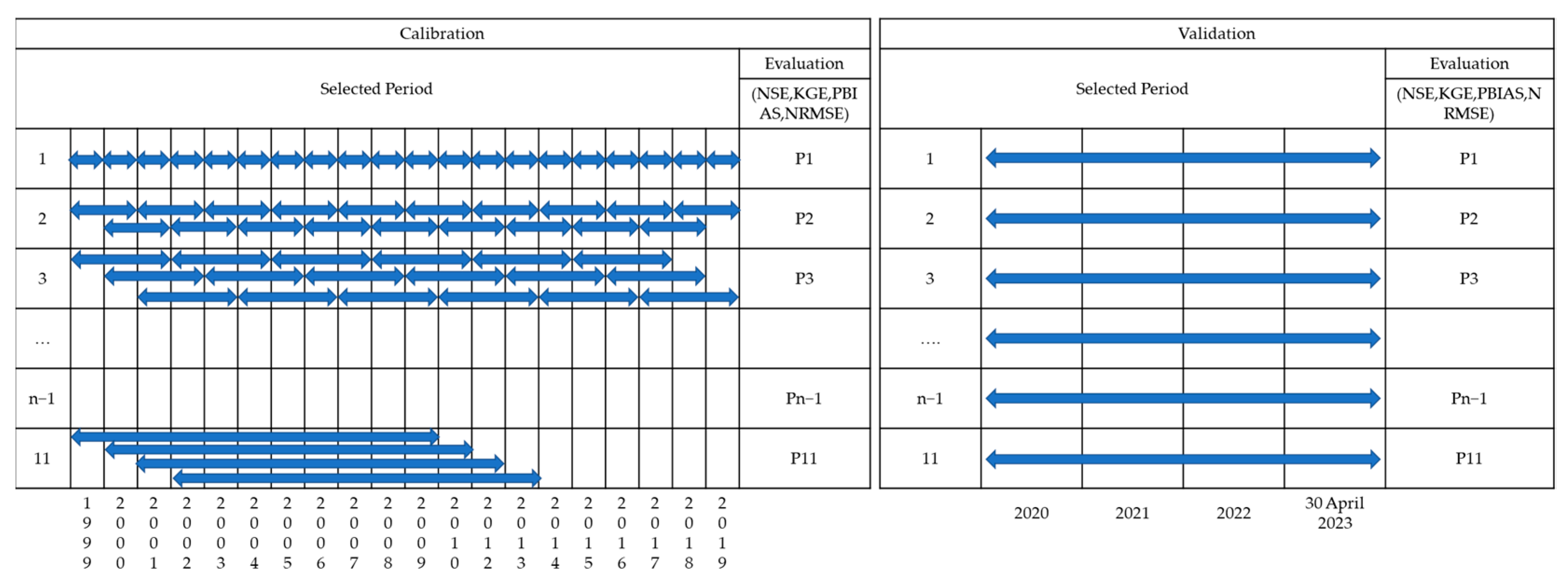
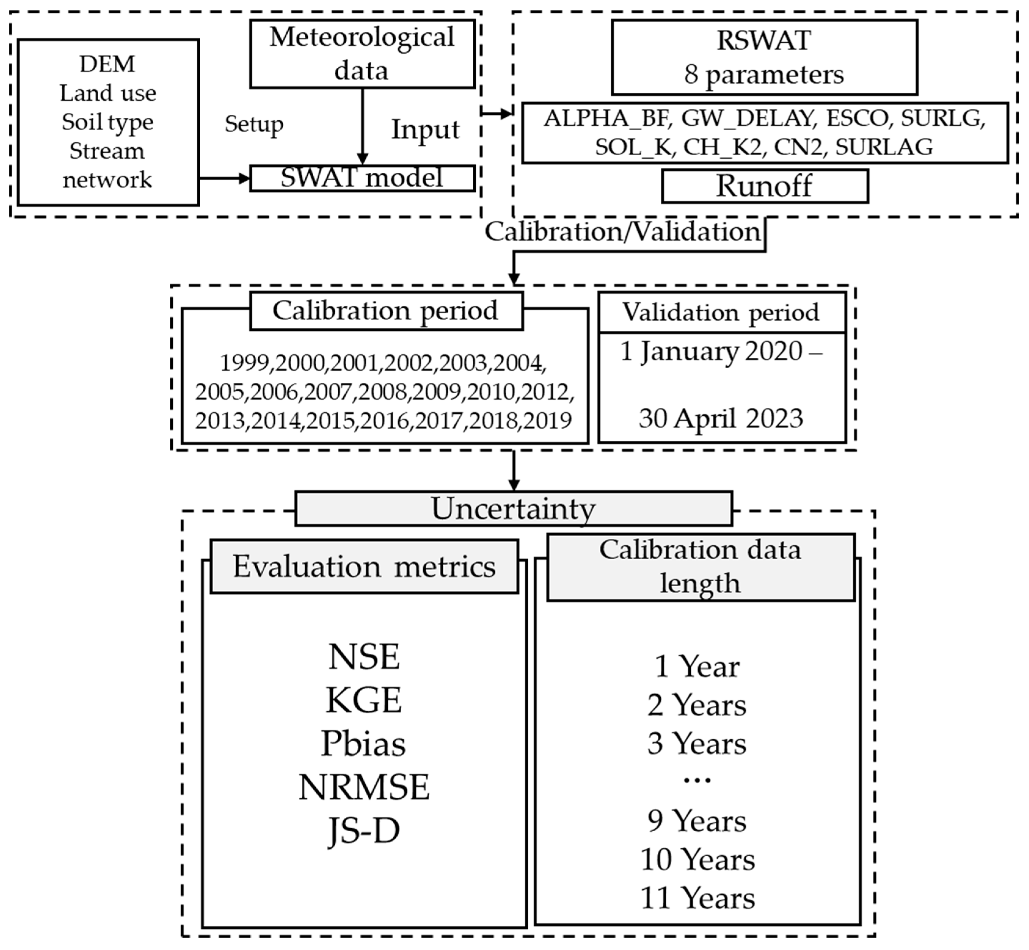
2.1. Study Procedure

Figure 1 shows the workflow for quantifying the uncertainty in runoff simulations according to the selection of evaluation metrics and calibration data length. First, topographic and meteorological data were constructed to perform runoff simulations using the SWAT model. Then, among the parameters of the SWAT model, parameters related to groundwater, soil, channel routing, etc., were selected to perform SWAT model parameter optimization using the R-SWAT. Next, two forms of uncertainty in the runoff simulations were quantified to (1) analyze the uncertainty as quantified by different evaluation metrics and (2) analyze the uncertainty of simulated runoff according to different calibration data lengths.

2.2. Geospatial Data

The study was carried out in the Yeongsan River upper basin, located in Korea’s southwestern region, encompassing the latitude bracket of 35.7°–35.5° and the longitude span of 126.4°–127.1°. The basin area is approximately 3371.4 km² in total, as shown in Figure 2. The region’s average annual temperature is noted to be 14.0 °C with an annual rainfall reaching up to 1293 mm. The region’s landscape is made up of 45.4% forests, 35.5% farmlands, 7.3% urbanized zones, 5.2% grasslands, 3.4% water bodies, 1.8% barren lands, and 1.4% wetlands. The Yeongsan River basin has an average annual runoff of 22.9 m³/s, with a standard deviation of 6.77, and a standard deviation to mean ratio of 0.29, indicating a relatively stable hydrological system. The maximum daily runoff was recorded during the significant Korean Peninsula heavy rainfall event in August 2020, reaching 2917.7 m³/s, and the maximum monthly runoff in August 2020 was 184.5 m³/s. The runoff of the Yeongsan River basin during historical periods is shown in Figure S1. The largest urban region in the study area is Gwangju Metropolitan City, and the water from the Yeongsan River basin is harnessed for irrigation and household needs. Despite its considerable size, the basin is relatively unimpacted by man-made constructions like dams. However, the Yeongsan River does not have sufficient river runoff in the dry season, which has led to frequent extreme droughts, especially in the late 2000s and 2014–2015.

In this study, Thiessen polygons were generated based on the locations of meteorological stations managed by the Korea Meteorological Administration. Subsequently, six meteorological stations (Gwangju, Haenam, Jangheung, Jeongeup, Mokpo, and Namwon) overlapping with the study area were selected. For runoff data, the water level station (Geukrak) was chosen due to its comprehensive data availability compared to other stations in the Yeongsan River basin.

2.3. Soil and Water Assessment Tool (SWAT) Model

The calibration of the hydrological model according to the different calibration data lengths in the study basin was evaluated using the SWAT model. The SWAT model is a physically based semi-distributed model and has been widely used for runoff, non-point-source pollution, and other complex hydrological processes under changing environments [28]. It benefits from the capability to model watershed hydrologic processes using relatively straightforward input variables. In addition, the SWAT model has often been utilized in recent studies of the Yeongsan River basin in South Korea [9,29]. The hydrological cycle of the SWAT model is simulated based on the water balance equation, as shown in Equation (1).

$${SW}_t={SW}_0+\sum _{i=0}^t\left(R_{day}-Q_{surf}-E_a-w_{seep}-Q_{gw}\right)$$

(1)

where ${SW}_0$ is the initial soil moisture content (mm), ${SW}_t$ is the total soil moisture per day (mm), $R_{day}$ is precipitation (mm), $Q_{surf}$ is surface runoff (mm), $E_a$ is evapotranspiration (mm), $W_{seed}$ is penetration, $Q_{gw}$ is groundwater runoff (mm), and $t$ is time (day).

In this study, QSWAT3 v1.65 was employed for runoff analysis using climate data, and R-SWAT [30] was used for the parameter optimization of the SWAT model. R-SWAT contains the SUFI-2 algorithm, which is well known for its fast performance with high accuracy for parameter optimization [31]. In this study, SWAT parameter optimization was performed using the SUFI-2 algorithm of R-SWAT. For SWAT parameter optimization, several studies [32,33,34] have mainly recommended performing more than 500 iterations. Consequently, parameters were optimized through 1000 iterations uniform for each case. The calibration time on a CPU with 20 cores took 2 h per 1000 iterations.

2.4. Hydrological Model Parameter Calibration

To quantify the uncertainty according to the calibration data length, the calibration data lengths were divided into 11 cases, as shown in Figure 3. The calibration data length was increased by one to 11 years for the 21-year period from 1999 to 2019, and SWAT parameter optimization was performed. Note that there were no observational data for 2011 because of large-scale civil works in the basin; therefore, 2011 was neglected in the calibration data length. The water level station (Geukrak) used in this study was located in the upper basin of the Yeongsan River, and therefore, it was not influenced by these large-scale civil works. To obtain appropriate calibration and validation results irrespective of which calibration data length was selected, all possible calibration periods were considered [25]. As illustrated in Figure 3, the calibration and validation stages of each experiment were distinctly separated with no overlaps. Based on this independence, the calibration and validation processes were appropriate for use in split-sample tests [35]. Then, the evaluation metrics for the validation period were calculated using the simulated and observed runoff data from 1 January 2020 to 30 April 2023.

2.5. Uncertainty Assessment

Various evaluation metrics were used to quantify the uncertainty of the simulated runoff based on the calibration data length. First, the NSE is often used in hydrological studies to evaluate the performance of simulated data reproducing the observed data. The NSE evaluates the difference between the extreme values of the observed and simulated data and the average values using Equation (2). Thus, this model can evaluate the simulation of extreme runoff values. Second, the KGE metric, as shown in Equation (3), was employed to evaluate the spatial dispersion between the observed and simulated data. Lastly, Pbias and NRMSE were computed using Equations (4) and (5) to evaluate the deviation between the observed and simulated data, and the error between the observed and simulated data, respectively.

$$NSE=1-\frac{\sum _{i=1}^n{(X_s-X_o)}^2}{\sum _{i=1}^n{(X_o-\overline{X_o})}^2}$$

(2)

$$KGE=1-\sqrt{{(r-1)}^2+{(\alpha -1)}^2+{(\beta -1)}^2}$$

(3)

$$Pbias=\frac{\sum _{i=1}^n(X_o-X_s)}{\sum _{i=1}^n{X}_o}$$

(4)

$$NRMSE=\frac{\sqrt{\frac{1}{n}{\sum }_{i=1}^n{(X_s-X_o)}^2}}{{\overline{X}}_O}$$

(5)

where $X_S$ is the simulated data, $X_o$ is the observed data, $n$ is the total number of data, $\overline{X_o}$ is the average of observed data, $r$ is the correlation coefficient between the observed and simulated value, $\alpha$ is the relative variability in the observed and simulated value, and $\beta$ is the bias term.

To ensure consistency among the evaluation metrics, NSE and KGE were min–max normalized according to Equation (6). The absolute values of Pbias and NRMSE were also min–max normalized. In this normalization, the higher the value, the greater the uncertainty, as described in Equation (7). Each evaluation metric was assigned an equal weight.

$$x_{normalized}=\frac{x-x_{max}}{x_{min}-x_{max}}$$

(6)

$$x_{normalized}=\frac{x-x_{min}}{x_{max}-x_{min}}$$

(7)

where $x$ is the evaluation metrics.

An uncertainty index was then calculated using the four evaluation metrics to quantify the overall uncertainty, as shown in Equation (8):

$$Uncertaintyindex={\frac{1}{4}NSE}_{normalized}+{\frac{1}{4}KGE}_{normalized}+{\frac{1}{4}AbsPbias}_{normalized}+{\frac{1}{4}NRMSE}_{normalized}$$

(8)

To determine the uncertainty in simulating extreme runoff events that exceeded the 95th percentile, Jensen–Shannon divergence (JS-D) was used to compare the simulated and observed runoff data. JS-D offers a method to assess the degree of similarity or difference between two probability distributions without the need for statistical moments. As a finite, nonnegative, and bounded metric, JS-D quantifies the divergence between distinct probability distributions [36]. JS-D was defined to resolve the limitations of Kullback–Leibler divergence (KL-D), particularly for simplistic distributions [37]. KL-D measures the entropy loss of a probability density function (PDF), making it less suitable for simple distributions [38]. Equation (9) provides the formula for KL-D, which quantifies the information loss that occurs when the PDF of $Y$ is substituted with that of $X$:

$$D_{KL}\left(X\left|\right|Y\right)=\sum _{x\in X}^P\log \frac{p\left(x_i\right)}{p\left(y_i\right)}$$

(9)

where $p\left(x_i\right)$ and $p\left(y_i\right)$ are the probabilities that $X$ and $Y$ are, respectively, in the states $x_i$ and $y_i$.

According to Equation (9), the sums of the KLD of $\left(X\left|\right|Y\right)$ and $\left(Y\left|\right|X\right)$ are calculated and made symmetrical. In its general form for $N$ distributions, $J_{KL}$ divergence can be expressed as in Equation (10).

$$J_{KL}=\sum _{i=1}^N\left(X_i\left|\right|Y_i\right)$$

(10)

Then, JSD is developed by comparing each distribution to the “midpoint” distribution, $M$, defined in Equation (11):

$$M=\frac{1}{N}\sum _{i=1}^N\left(X_i+Y_i\right)$$

(11)

Accordingly, JSD represents the average divergence of $N$ probability distributions from their midpoint distribution, as defined in Equation (12):

$$JSD=\frac{1}{N}\sum _{i=1}^N{D}_{KL}\left(X_i\left|\right|M\right)$$

(12)

Thus, JS-D can measure the similarity between the two distributions.

3. Results

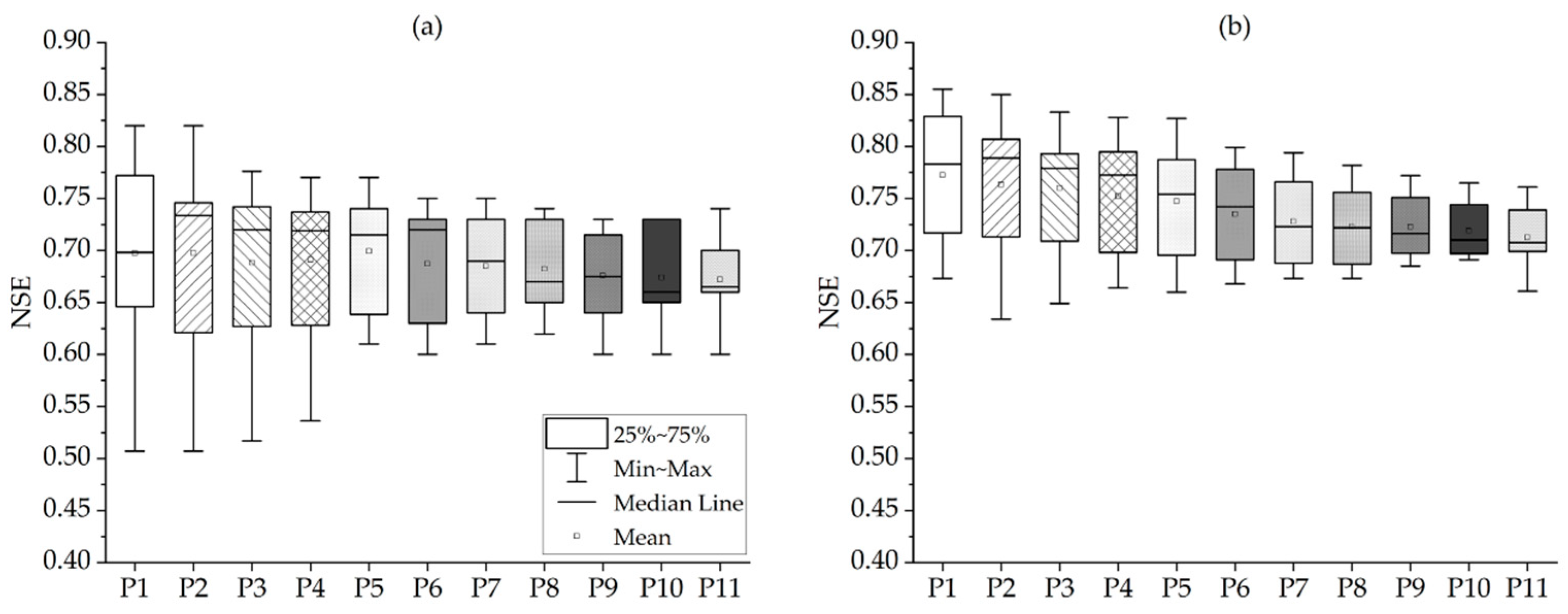
3.1. Model Performance over the Calibration Period

The SWAT model parameters that reflect the groundwater, hydrologic response unit, watershed, and soil characteristics were selected. The selected parameters, including their boundary conditions, are listed in Table S1. Parameter optimization was performed using R-SWAT by setting the objective function to NSE. The box plots of the model’s performance before and after calibration are shown in Figure 4 and

Table 1. Statistics of NSEs in each calibration period.

Calibration	Criteria	P1	P2	P3	P4	P5	P6	P7	P8	P9	P10	P11	Avg.
Before	25%	0.649	0.630	0.631	0.630	0.640	0.638	0.640	0.653	0.650	0.650	0.660	0.643
	75%	0.771	0.743	0.742	0.736	0.730	0.730	0.730	0.723	0.700	0.708	0.690	0.727
	IQR	0.122	0.113	0.110	0.107	0.090	0.093	0.090	0.070	0.050	0.058	0.030	0.085
After	25%	0.719	0.714	0.722	0.705	0.697	0.693	0.690	0.690	0.704	0.701	0.702	0.703
	75%	0.819	0.806	0.791	0.794	0.784	0.777	0.761	0.754	0.744	0.734	0.726	0.772
	IQR	0.100	0.092	0.069	0.089	0.087	0.084	0.072	0.064	0.040	0.033	0.024	0.069

. Each box plot was generated based on the calibrated period according to the calibration data length. As a result of the parameter optimization, the NSE was more than 0.65 in all cases, showing that the results of the SWAT model can be considered reasonable. The performances of all optimized parameter sets are different according to each period, even if the calibration data length is the same. In other words, the higher the evaluation metrics value and the smaller the value of the interquartile range (IQR), the lower the uncertainty.

The IQR, which represents the model uncertainty in the calibration period, was the largest for P1 before and after calibration, at 0.122 and 0.100, and the smallest for P11, at 0.030 and 0.024. The shorter the calibration data length, the higher the model performance but the higher the inherent uncertainty of each independent period. The average IQR for the NSE, including all calibration data lengths, decreased from 0.085 to 0.069 after calibration, and showed a decrease in uncertainty.

3.2. Evaluation of Performance over Validation Period

The overall hydrologic graph during the validation period is shown in Figure S2. With the exception of an extreme runoff event in August 2020 due to heavy rains on the Korean Peninsula, the simulated daily runoff followed the trend of the observed runoff data, with similar seasonal variability. The results of the evaluation metrics for the validation period according to different calibration data lengths are shown in Figure 5 and Table S2. The uncertainty according to the evaluation metrics and calibration data length was described in each evaluation metric as the average value due to the calibration data length. A general concept of each evaluation metric can be set out as follows: the closer the NSE and KGE are to 1, the lower the uncertainty, and the closer the Pbias and NRMSE are to 0, the lower the uncertainty. Uncertainty based on evaluation metric values differs for each evaluation metric, but uncertainty based on IQR has higher uncertainty with larger IQR values. The average value of NSE in the validation period was 0.71, which was higher than in the calibration period. The average value was the highest (0.74) in P5 and the lowest (0.72) in P1, which means that the uncertainty based on the average value was the highest in P1 and the lowest in P5. The IQR value was the highest (0.05) in P1 and the lowest (0.01) in P7 and P11, which means that the uncertainty based on the NSE value was highest. The average value of KGE was the highest (0.61) in P5 and the lowest (0.59) in P11, indicating the highest uncertainty in P11. The IQR value of KGE had the highest value (0.09) in P1 and the lowest value (0.03) in P7, P9, and P11.

The average value of the absolute Pbias was the lowest in P6 (2.84) and the highest in P8 (4.36), with the highest uncertainty in P8. The IQR of Pbias was the highest in P1 (4.03) and the lowest in P2 and P5 (2.00). NRMSE was the lowest for P5 (51.08), and the IQR was the highest for P1 (3.73). Considering the average, the uncertainty in the NRMSE was the largest for P1 (52.52).

Overall, the uncertainty based on the average value of each evaluation metric varied depending on the evaluation metric. NSE and NRMSE have higher uncertainties for shorter calibration data lengths, while KGE and Pbias have higher uncertainties for longer calibration data lengths. Consistently, P5 to P7 have lower uncertainties. The uncertainty based on IQR values was found to be the highest for P1 for all evaluation metrics, while P7 was evaluated as having relatively low uncertainty.

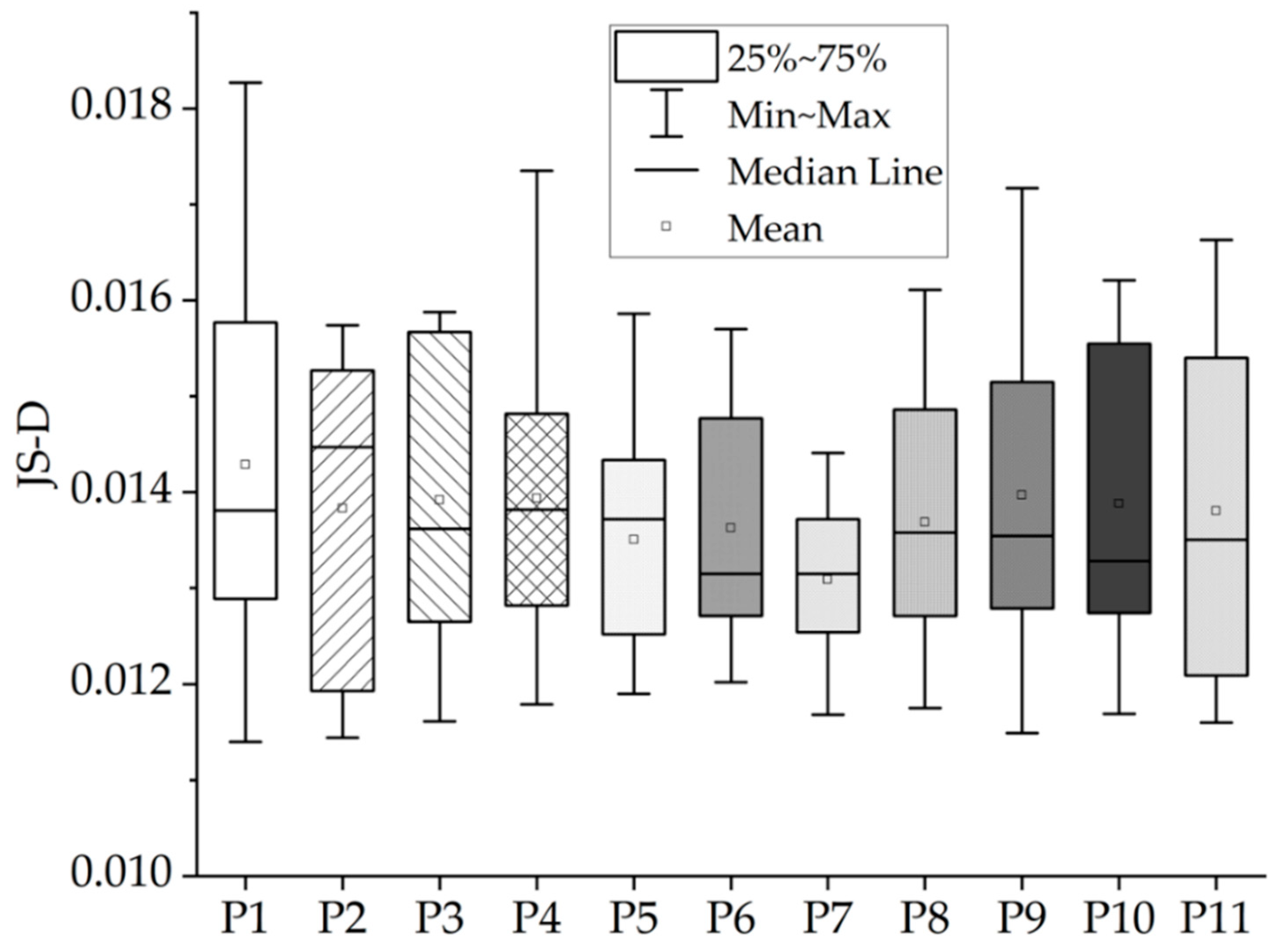
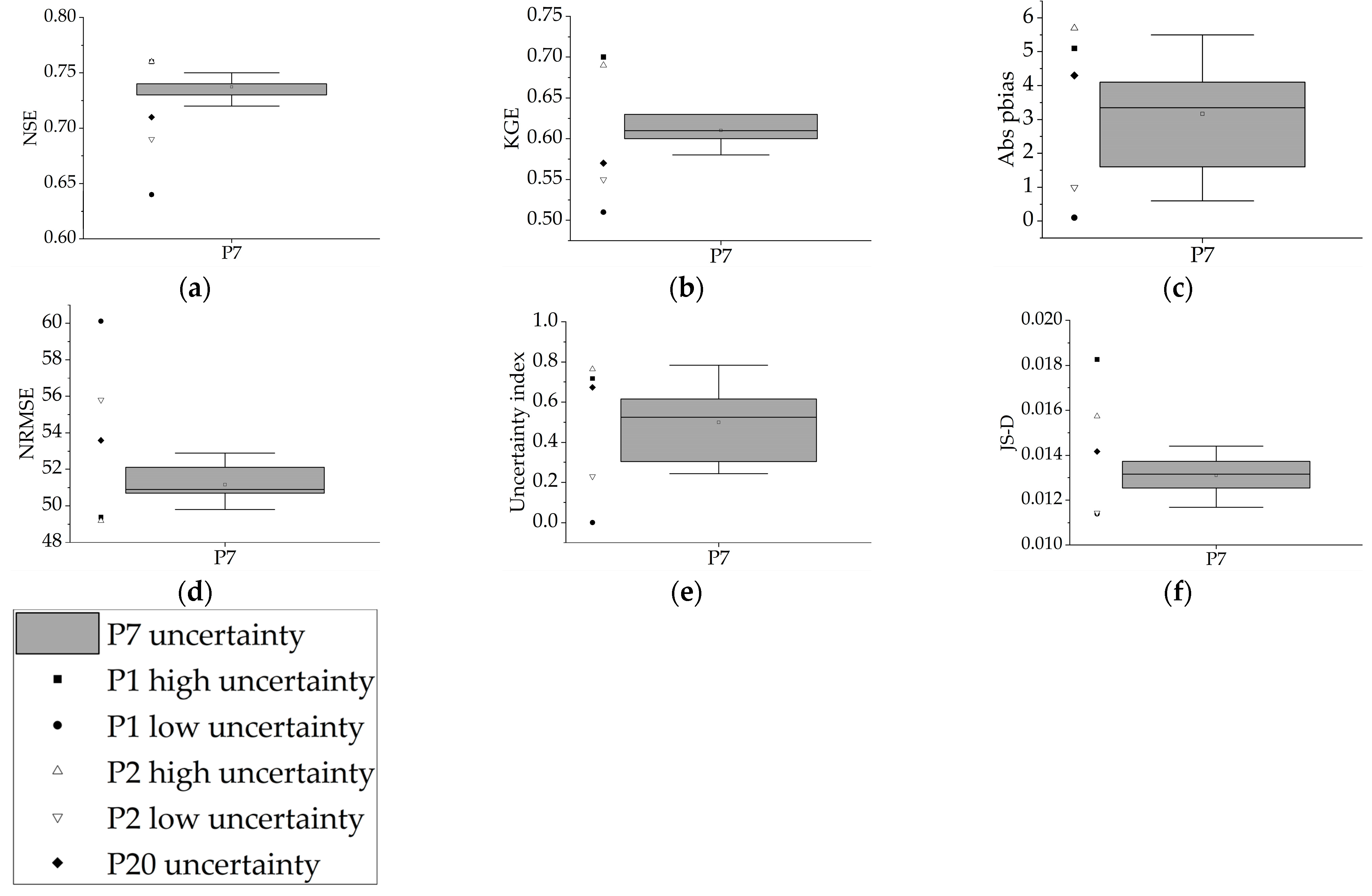
3.3. Uncertainty Index

The uncertainty index was calculated using the evaluation metrics presented in Figure 6 and

Table 2. Statistics of uncertainty index in validation period.

	P1	P2	P3	P4	P5	P6	P7	P8	P9	P10	P11
Avg.	0.385	0.343	0.311	0.352	0.329	0.327	0.350	0.387	0.398	0.454	0.430
Median	0.340	0.357	0.305	0.341	0.327	0.316	0.366	0.373	0.398	0.458	0.425
25%	0.287	0.237	0.217	0.277	0.277	0.250	0.287	0.284	0.312	0.390	0.385
75%	0.469	0.404	0.390	0.384	0.401	0.402	0.419	0.465	0.476	0.504	0.491
IQR	0.181	0.167	0.173	0.107	0.124	0.152	0.132	0.181	0.163	0.114	0.105

. The uncertainty index was calculated by conducting the min–max normalization of each evaluation metric, where a value closer to 1 indicates greater uncertainty in the runoff simulation. The calculated uncertainty index was the highest for P10 (0.454), while P3 had a low uncertainty, with an average of 0.311. The difference in the length of each calibration period was the highest for P1, with an IQR of 0.181, and the lowest for P11, with an IQR of 0.11. The median value of the uncertainty index also indicated that P3 had the lowest uncertainty, at 0.305, whereas P10 had the highest uncertainty, at 0.458. The maximum value of uncertainty index for P5–7was calculated to be lower compared to the average value of 0.552 (P5—0.425, P6—0.519, and P7—0.448). In particular, the maximum values for P5 and P7 show significantly lower uncertainty compared to other calibration period lengths.

3.4. Evaluation of the Extreme Runoff

To analyze the uncertainty of the extreme runoff simulations, the 98th–100th percentiles of observed and simulated runoff were compared. Overall, the simulated runoff for the 98–100 percentiles performed similarly to the observed extreme runoff, as shown in Figure S3. JS-D was then used to calculate the similarity between the observed and simulated extreme runoff distributions, as shown in Figure 7 and Table S3. The higher the value of JS-D, the higher the difference between the two distributions. Here, the higher the value of JS-D, the higher the uncertainty in simulated extreme runoff. It was found that JS-D for P1 had the greatest uncertainty, with an average of 0.0143, whereas that of P7 was the smallest, with an average of 0.0131. The median values of JS-D also showed that P6 and P7 had the lowest uncertainty, at 0.0132, whereas P2 had the highest, at 0.0145.

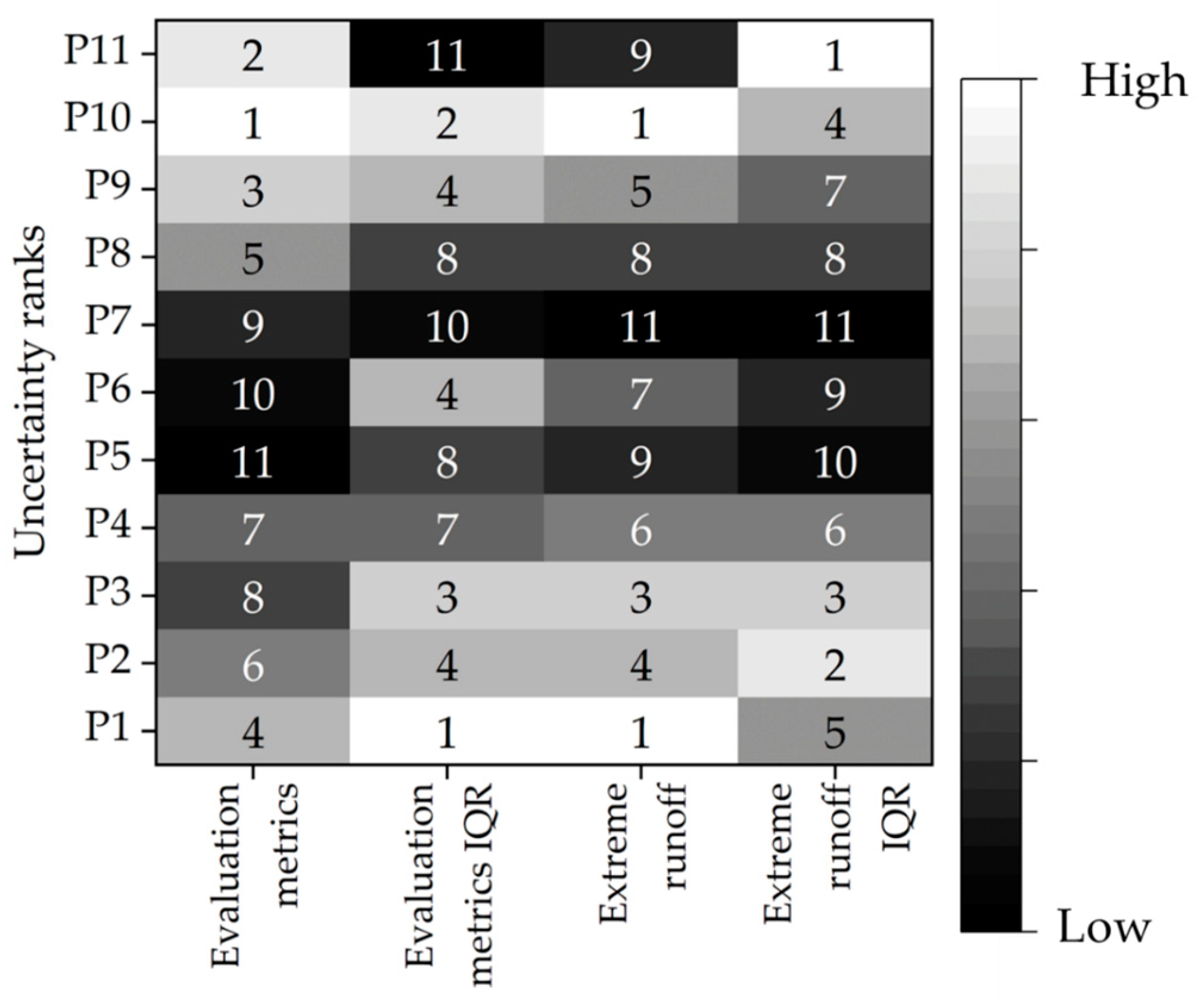
3.5. Overall Uncertainty Assessment

The overall uncertainty rankings are shown in Figure 8. In this matrix chart, a higher ranking—with 1 being the highest—indicates greater uncertainty. Thus, the overall uncertainty was lower for runoff simulations with calibration data lengths of five to seven years, with that of P7 being the lowest. In particular, P7 had the lowest uncertainty according to the calibration data length for the extreme runoff simulations. For a period longer than P7, the uncertainty was higher, but the uncertainty based on the IQR was relatively low. This suggests that there is an optimal length for the calibration period, and an excessive amount of data might have heightened the uncertainty in the runoff simulations.

4. Discussion

Hydrological models have been popularly used in water management because the runoff can be simulated using climate data, where observational runoff data are lacking. In addition, hydrological models that consider terrain data reflecting the characteristics of a region provide more reliable simulations. However, to use the simulation data of a hydrological model, it is necessary to optimize the model parameters using the observed runoff data. However, there is some degree of uncertainty in the parameter calibration process. This uncertainty sometimes has significant implications for water resource management and planning [39,40,41].

As shown in Figure 5, the selection of evaluation metrics has a significant impact on the degree of uncertainty. As a result, the uncertainty in the runoff simulations was quantified using different evaluation metrics in this study. The results for NSE and NRMSE were consistent with existing studies, in that short calibration data lengths do not reflect various hydrological cycle conditions, resulting in large uncertainties in the runoff simulations. In contrast, KGE and Pbias showed large uncertainties when the hydrological model parameters with relatively long calibration data lengths were used. This is consistent with previous studies that have characterized NSE as giving more importance to correlation than bias, and that bias and variance can be more easily distinguished when compared using KGE [42]. This confirms that there is some degree of uncertainty using only one or two metrics, and thus a variety of metrics should be considered at the parameter calibration in hydrologic modeling [43].

Contrary to the common assumption that the longer the calibration data length, the lower the uncertainty of runoff simulations when optimizing hydrologic model parameters, the results of this study show that the optimal calibration data length is five to seven years, with the lowest uncertainty obtained with a data length of seven years (P7). This result is similar to previous research in the same region of Korea [25], which found that a calibration data length of six to eight years provides reliable runoff simulation, but differs from studies that generally recommend using a calibration data length of eight years or more [20,23].

To compare with the common assumption that longer calibration data lengths are advantageous for optimizing parameters of hydrological models, this study conducted a comparative analysis using a parameter set calibrated with the maximum observed length of 20 years in the Yeongsan River basin. Consequently, to analyze the uncertainty with more detailed calibration data lengths, the analysis was performed using a calibration data length of P20, which was 20 years long and considered all periods of observed runoff data. For a contrasting analysis, the highest and the lowest uncertainty cases of the shorter calibration data lengths, P1 of one year and P2 of two years, were considered together. The results of the comparative analysis with P7, which has the lowest overall uncertainty in this study, are shown in Figure 9. P20 has higher uncertainty than P7 in all cases of NSE, KGE, Pbais, NRMSE, uncertainty index, and JS-D. This supports the idea that a data length longer than the optimal calibration data length found in this study actually increases uncertainty. For P1 and P2, with shorter calibration data lengths, the lower uncertainty cases showed lower uncertainty than P7, but the higher uncertainty cases all had higher uncertainty than P7. This means that shorter calibration data lengths may have performance and uncertainty benefits for runoff simulation in some cases, but the individual uncertainties for each period are high, resulting in large deviations. This confirms the need to use different combinations of observed runoff data in runoff simulations using hydrological models when the length of the observed runoff data is short or the data lacks continuity.

This study has immediate applications in policy decisions and water management practices. Water resource managers and policymakers could employ the insights gained to optimize calibration lengths and evaluation metrics, thus enhancing model reliability. The methodological approach of using multiple evaluation metrics to quantify uncertainty represents a significant advancement in hydrological studies. Moreover, the results are particularly useful for locations where data may be scarce or incomplete, as demonstrated by the model’s performance despite missing data for 2011. However, there are some limitations that should be highlighted. While this study provides specific insights into the Yeongsan River basin, the methodology and findings offer broader implications for hydrological modeling. The approach to determining the optimal calibration data length, based on a balance between reducing uncertainty and the practicality of data availability, can be applied to other river basins. However, it is important to note that the specific optimal calibration period may vary depending on several factors, including the hydrological characteristics of the basin, the variability of meteorological conditions, and the quality and quantity of available data. Therefore, while our study findings suggest a general approach to identifying an optimal calibration data length, this study recommends that hydrologists and modelers conduct similar analyses tailored to their specific river basins. Such analyses should consider local hydrological dynamics and data characteristics to determine the most appropriate calibration period for their models.

5. Conclusions

The uncertainty of runoff simulations using climate data and a hydrological model in the Yeongsan River Basin located in southwest South Korea was quantified. The uncertainty of the runoff simulations was considered based on the calibration data length and the selection of the evaluation metrics. To quantify the uncertainty of the runoff simulation, and the extreme runoff (95th percentile flow), the difference in performance according to the calibration data length, and the difference in performance according to the validation period were quantified. Extreme runoff was evaluated using JS-D to determine the difference in the distribution from the observed data, and NSE, KGE, Pbias, and NRMSE were applied as the evaluation metrics. Based on the results, the following conclusions can be drawn:

• Different evaluation metrics all showed different levels of uncertainty, which means it is necessary to consider multiple evaluation metrics rather than relying on any one single metric;
• Runoff simulations using a hydrological model had the least uncertainty owing to the calibration data length when using a parameter set of seven years, and the uncertainty increased for calibration data lengths longer than seven years;
• Parameter sets with the same calibration length showed period-dependent uncertainty, which led to uncertainty differences within the same length;
• For extreme runoff simulations, employing long calibration data lengths (of more than seven years) achieved lower uncertainty than shorter calibration data lengths.

In the end, this study contributes to the broader knowledge base by providing a framework for assessing the optimal calibration data length in hydrological modeling. This framework can be adapted and applied to other river basins, with the understanding that local conditions and data availability will influence the specific outcomes.

References

1. Beven, K. Linking parameters across scales: Subgrid parameterizations and scale dependent hydrological models. Hydrol. Process 1995, 9, 507–525. [Google Scholar] [CrossRef]
2. Harmel, R.D.; Smith, P.K. Consideration of measurement uncertainty in the evaluation of goodness-of-fit in hydrologic and water quality modeling. J. Hydrol. 2007, 337, 326–336. [Google Scholar] [CrossRef]
3. He, Y.; Bárdossy, A.; Zehe, E. A review of regionalisation for continuous streamflow simulation. Hydrol. Earth Syst. Sci. 2011, 15, 3539–3553. [Google Scholar] [CrossRef]
4. Moges, E.; Demissie, Y.; Larsen, L.; Yassin, F. Review: Sources of hydrological model uncertainties and advances in their analysis. Water 2020, 13, 28. [Google Scholar] [CrossRef]
5. Wang, X.; Yang, T.; Wortmann, M.; Shi, P.; Hattermann, F.; Lobanova, A.; Aich, V. Analysis of multi-dimensional hydrological alterations under climate change for four major river basins in different climate zones. Clim. Change 2017, 141, 483–498. [Google Scholar] [CrossRef]
6. Arsenault, R.; Brissette, F.; Martel, J.L. The hazards of split-sample validation in hydrological model calibration. J. Hydrol. 2018, 566, 346–362. [Google Scholar] [CrossRef]
7. Troin, M.; Arsenault, R.; Martel, J.L.; Brissette, F. Uncertainty of hydrological model components in climate change studies over two Nordic Quebec catchments. J. Hydrometeorol. 2018, 19, 27–46. [Google Scholar] [CrossRef]
8. Gong, W.; Gupta, H.V.; Yang, D.; Sricharan, K.; Hero III, A.O. Estimating epistemic and aleatory uncertainties during hydrologic modeling: An information theoretic approach. Water Resour. Res. 2013, 49, 2253–2273. [Google Scholar] [CrossRef]
9. Song, Y.H.; Chung, E.S.; Shahid, S. Differences in extremes and uncertainties in future runoff simulations using SWAT and LSTM for SSP scenarios. Sci. Total Environ. 2022, 838, 156162. [Google Scholar] [CrossRef] [PubMed]
10. Hu, J.; Zhou, Q.; McKeand, A.; Xie, T.; Choi, S.K. A model validation framework based on parameter calibration under aleatory and epistemic uncertainty. Struct. Multidiscipl. Optim. 2021, 63, 645–660. [Google Scholar] [CrossRef]
11. Clark, M.P.; Nijssen, B.; Lundquist, J.D.; Kavetski, D.; Rupp, D.E.; Woods, R.A.; Freer, J.E.; Gutmann, E.D.; Wood, A.W.; Gochis, D.J.; et al. A unified approach for process-based hydrologic modeling: Part 1. Modeling concept. Water Resour. Res. 2015, 51, 2498–2514. [Google Scholar] [CrossRef]
12. Van der Spek, J.E.; Bakker, M. The influence of the length of the calibration period and observation frequency on predictive uncertainty in time series modeling of groundwater dynamics. Water Resour. Res. 2017, 53, 2294–2311. [Google Scholar] [CrossRef]
13. Myers, D.T.; Ficklin, D.L.; Robeson, S.M.; Neupane, R.P.; Botero-Acosta, A.; Avellaneda, P.M. Choosing an arbitrary calibration period for hydrologic models: How much does it influence water balance simulations? Hydrol. Process 2021, 35, e14045. [Google Scholar] [CrossRef]
14. Razavi, S.; Tolson, B.A. An efficient framework for hydrologic model calibration on long data periods. Water Resour. Res. 2013, 49, 8418–8431. [Google Scholar] [CrossRef]
15. Perrin, C.; Oudin, L.; Andreassian, V.; Rojas-Serna, C.; Michel, C.; Mathevet, T. Impact of limited streamflow data on the efficiency and the parameters of rainfall—Runoff models. Hydrol. Sci. J. 2007, 52, 131–151. [Google Scholar] [CrossRef]
16. Motavita, D.F.; Chow, R.; Guthke, A.; Nowak, W. The comprehensive differential split-sample test: A stress-test for hydrological model robustness under climate variability. J. Hydrol. 2019, 573, 501–515. [Google Scholar] [CrossRef]
17. Sorooshian, S.; Gupta, V.K.; Fulton, J.L. Evaluation of maximum likelihood parameter estimation techniques for conceptual rainfall-runoff models: Influence of calibration data variability and length on model credibility. Water Resour. Res. 1983, 19, 251–259. [Google Scholar] [CrossRef]
18. Harlin, J. Development of a process oriented calibration scheme for the HBV hydrological model. Hydrol. Res. 1991, 22, 15–36. [Google Scholar] [CrossRef]
19. Refsgaard, J.C.; Knudsen, J. Operational validation and intercomparison of different types of hydrological models. Water Resour. Res. 1996, 32, 2189–2202. [Google Scholar] [CrossRef]
20. Yapo, P.O.; Gupta, H.V.; Sorooshian, S. Automatic calibration of conceptual rainfall-runoff models: Sensitivity to calibration data. J. Hydrol. 1996, 181, 23–48. [Google Scholar] [CrossRef]
21. Anctil, F.; Perrin, C.; Andréassian, V. Impact of the length of observed records on the performance of ANN and of conceptual parsimonious rainfall-runoff forecasting models. Environ. Model. Softw. 2004, 19, 357–368. [Google Scholar] [CrossRef]
22. Vaze, J.; Post, D.A.; Chiew, F.H.S.; Perraud, J.M.; Viney, N.R.; Teng, J. Climate non-stationarity–validity of calibrated rainfall–runoff models for use in climate change studies. J. Hydrol. 2010, 394, 447–457. [Google Scholar] [CrossRef]
23. Kim, H.S.; Croke, B.F.; Jakeman, A.J.; Chiew, F.H. An assessment of modelling capacity to identify the impacts of climate variability on catchment hydrology. Math. Comput. Simul. 2011, 81, 1419–1429. [Google Scholar] [CrossRef]
24. Jin, J.; Zhang, Y.; Hao, Z.; Xia, R.; Yang, W.; Yin, H.; Zhang, X. Benchmarking data-driven rainfall-runoff modeling across 54 catchments in the Yellow River Basin: Overfitting, calibration length, dry frequency. J. Hydrol. Reg. Stud. 2022, 42, 101119. [Google Scholar] [CrossRef]
25. Shin, M.J.; Jung, Y. Using a global sensitivity analysis to estimate the appropriate length of calibration period in the presence of high hydrological model uncertainty. J. Hydrol. 2022, 607, 127546. [Google Scholar] [CrossRef]
26. Noor, M.; Ismail, T.B.; Shahid, S.; Ahmed, K.; Chung, E.S.; Nawaz, N. Selection of CMIP5 multi-model ensemble for the projection of spatial and temporal variability of rainfall in peninsular Malaysia. Theor. Appl. Climatol. 2019, 138, 999–1012. [Google Scholar] [CrossRef]
27. Raju, K.S.; Kumar, D.N. Review of approaches for selection and ensembling of GCMs. J. Water Clim. Change 2020, 11, 577–599. [Google Scholar] [CrossRef]
28. Arnold, J.G.; Srinivasan, R.; Muttiah, R.S.; Williams, J.R. Large area hydrologic modeling and assessment part I: Model development 1. J. Am. Water Resour. Assoc. 1998, 34, 73–89. [Google Scholar] [CrossRef]
29. Kim, J.H.; Sung, J.H.; Shahid, S.; Chung, E.S. Future hydrological drought analysis considering agricultural water withdrawal under SSP scenarios. Water Resour. Manag. 2022, 36, 2913–2930. [Google Scholar] [CrossRef]
30. Nguyen, T.V.; Dietrich, J.; Dang, T.D.; Tran, D.A.; Van Doan, B.; Sarrazin, F.J.; Abbaspour, K.; Srinivasan, R. An interactive graphical interface tool for parameter calibration, sensitivity analysis, uncertainty analysis, and visualization for the Soil and Water Assessment Tool. Environ. Model. Softw. 2022, 156, 105497. [Google Scholar] [CrossRef]
31. Ahmed, N.; Wang, G.; Booij, M.J.; Xiangyang, S.; Hussain, F.; Nabi, G. Separation of the impact of landuse/landcover change and climate change on runoff in the upstream area of the Yangtze River, China. Water Resour. Manag. 2022, 36, 181–201. [Google Scholar] [CrossRef]
32. Yang, J.; Reichert, P.; Abbaspour, K.C.; Xia, J.; Yang, H. Comparing uncertainty analysis techniques for a SWAT application to the Chaohe Basin in China. J. Hydrol. 2008, 358, 1–23. [Google Scholar] [CrossRef]
33. Schuol, J.; Abbaspour, K.C. Calibration and uncertainty issues of a hydrological model (SWAT) applied to West Africa. Adv. Geosci. 2006, 9, 137–143. [Google Scholar] [CrossRef]
34. Kim, J.H.; Sung, J.H.; Chung, E.S.; Kim, S.U.; Son, M.; Shiru, M.S. Comparison of Projection in Meteorological and Hydrological Droughts in the Cheongmicheon Watershed for RCP4. 5 and SSP2-4.5. Sustainability 2021, 13, 2066. [Google Scholar] [CrossRef]
35. Klemeš, V. Operational testing of hydrological simulation models. Hydrol. Sci. J. 1986, 31, 13–24. [Google Scholar] [CrossRef]
36. Lin, J. Divergence measures based on the Shannon entropy. IEEE Trans. Inf. Theory 1991, 37, 145–151. [Google Scholar] [CrossRef]
37. Nicótina, L.; Alessi Celegon, E.; Rinaldo, A.; Marani, M. On the impact of rainfall patterns on the hydrologic response. Water Resour. Res. 2008, 44, W12401. [Google Scholar] [CrossRef]
38. Majtey, A.; Lamberti, P.W.; Martin, M.T.; Plastino, A. Wootters’ distance revisited: A new distinguishability criterium. Eur. Phys. J. D At. Mol. Opt. Phys. 2005, 32, 413–419. [Google Scholar] [CrossRef]
39. Bosshard, T.; Carambia, M.; Goergen, K.; Kotlarski, S.; Krahe, P.; Zappa, M.; Schär, C. Quantifying uncertainty sources in an ensemble of hydrological climate-impact projections. Water Resour. Res. 2013, 49, 1523–1536. [Google Scholar] [CrossRef]
40. Mockler, E.M.; Chun, K.P.; Sapriza-Azuri, G.; Bruen, M.; Wheater, H.S. Assessing the relative importance of parameter and forcing uncertainty and their interactions in conceptual hydrological model simulations. Adv. Water Resour. 2016, 97, 299–313. [Google Scholar] [CrossRef]
41. Zhou, S.; Wang, Y.; Li, Z.; Chang, J.; Guo, A. Quantifying the uncertainty interaction between the model input and structure on hydrological processes. Water Resour. Manag. 2021, 35, 3915–3935. [Google Scholar] [CrossRef]
42. Gupta, H.V.; Kling, H.; Yilmaz, K.K.; Martinez, G.F. Decomposition of the mean squared error and NSE performance criteria: Implications for improving hydrological modelling. J. Hydrol. 2009, 377, 80–91. [Google Scholar] [CrossRef]
43. Fowler, K.; Peel, M.; Western, A.; Zhang, L. Improved rainfall-runoff calibration for drying climate: Choice of objective function. Water Resour. Res. 2018, 54, 3392–3408. [Google Scholar] [CrossRef]
Figure 1. Study workflow.
Water 16 00517 g001
Figure 2. Study area.
Water 16 00517 g002
Figure 3. Description of the calibration data lengths and validation periods (The blue arrow means calibration data length).
Water 16 00517 g003
Figure 4. Variation in model performance (NSE) before (a) and after (b) parameter optimization. Numbers on the horizontal axis refer to the length of the calibration data used for parameter optimization.
Water 16 00517 g004
Figure 5. Box-plots of evaluation metrics for the validation period according to different calibration data lengths.
Water 16 00517 g005
Figure 6. Box-plot of uncertainty index for validation period.
Water 16 00517 g006
Figure 7. Difference between the simulated and the observed extreme runoff using JS-D.
Water 16 00517 g007
Figure 8. Matrix chart of overall uncertainty ranks.
Water 16 00517 g008
Figure 9. Overall uncertainty for long and short calibration data lengths together: (a)—NSE, (b)—KGE, (c)—Pbias, (d)—RMSE, (e)—uncertainty index, and (f)—JSD.
Water 16 00517 g009