A Methodology to Predict the Impact of a Marine Structure on Longshore Dynamics and Shoreline Evolution

Abstract

Globally, due to climate change and increased rates of coastal erosion, along with the need to protect sensitive habitats, there is an increasing requirement for a sustainable approach which considers both the effect of the marine environment on critical infrastructure and the impact of that infrastructure on the local environment. This paper presents a methodology for assessing the impact of a marine structure on longshore dynamics and shoreline evolution by using an external coupling of the phase-resolving ARTEMIS wave model and the shoreline evolution model, UNIBEST. The methodology can be applied at any coastal location, but for this study, it was applied to Sizewell Bay on the east coast of England to assess the impact of a shore-normal jetty on a gently curving stretch of shoreline with relatively complex offshore geomorphology. Results from simulating 22 years of shoreline evolution have shown that, at the jetty location, the shoreline at Sizewell will migrate seaward up to 45 m compared with the no-jetty case. Immediately south of the jetty, the shoreline was predicted to retreat landward by about 15 m. This behaviour is similar to observed changes at other locations, and the predicted longshore transport rates are in agreement with findings from previous studies, validating the methodology.

1. Introduction

Most new marine development remains at the coastal margin: increases in marine shipping have led to a worldwide expansion of ports, and increased tourism has produced expansion of coastal resorts. Throughout Europe, much recent research has focused on wind farms and their potential to provide beneficial environmental conditions as artificial reefs and inadvertent no-take zones, e.g., [1,2], while in the UK, the need for a secure and sustainable energy supply has resulted in several new major energy infrastructure developments. Such developments can be at risk of marine flooding or coastal erosion, with tools being developed to assess the risk due to the marine environment on the infrastructure, e.g., LISFLOOD [3]. However, there is a need to consider the impact of developments on the environment and with an emphasis on coastal erosion in particular.

The commensurate increases in protected areas, e.g., the Europe-wide UK Natura 2000 network, associated legislation such as the EU-wide Birds and Habitats Directives, and the need for continual infrastructure development, means that an overlap of impacts from developments and protected habitats becomes increasingly likely [4,5]. A sustainable approach which considers both infrastructure requirements and the sensitivities of the local environment is required.

From an engineering design and safety perspective, it is important to understand how new structures affect the immediate coastal hydrodynamics (waves and currents) but also to understand how these affect coastal sediment processes and shoreline or bathymetric change more widely. The objective of the present work is to develop and implement a new methodology to predict the impact of a hypothetical jetty construction (of substantial size, suitable for the transport of bulk building materials and very large loads) on longshore dynamics and shoreline evolution. The method includes the likely change in the sea bed and coastline in the direct vicinity of the development (scour due to waves and currents under the structure) and assesses the longshore extent of the zone of impact on coastal processes due to changes to the wave climate experienced in the lee of the jetty (extending over 100s of metres).

Scour is local and can be estimated with various empirical equations [6], while associated bathymetric change can affect the current and wave field, leading in turn to spatially variable changes in incident wave energy at the shoreline and gradients in longshore transport rate, which alter the spatial patterns of erosion or accretion.

Recent studies of shoreline evolution due to the actual or hypothetical construction of breakwaters/jetties or other marine structures have adopted different methodologies or techniques. The effect of a jetty construction on the updrift beach evolution in the south of Portugal has been evaluated by [7] based on several ortho-rectified aerial photographs and bathymetric maps. Ref. [8] have used a 26-year record of daily to hourly shoreline data adjacent to the jetty at Duck beach, North Carolina, extracted from video images, estimating the shoreline positions using a pixel analysis algorithm (this jetty’s configuration is similar to the structure proposed in Section 2.1 in this work, though with only two lines of support piles). Shoreline evolution has been modelled by [9] using the one-line shoreline evolution model UNIBEST [10], to predict the effect of a beach landing facility on shoreline evolution under various 20-year wave scenarios. Several studies have used directly coupled models:

• Ref. [11] investigated the impact of two hypothetical detached breakwaters on the shoreline evolution of the Portuguese West coast, using the CEDAS software package to directly couple the wave energy field calculated from STWAVE to the GENESIS model for calculating shoreline changes.
• Ref. [12] studied shoreline evolution due to the construction of two breakwaters on the West coast of India, using the MIKE 21 integrated model, which dynamically couples spectral-wave, hydrodynamic, sediment-transport and morphology modules.

By contrast, Ref. [13] used an external coupling of TELEMAC2D and ARTEMIS [14], where the velocity and wave results obtained by the respective model were combined in the same grid for post-processing, to examine the impact of shore-parallel breakwaters on the quasi-permanent tombolo deposits forming in their lee and wider shoreline evolution at Sea Palling on the north-east coast of Norfolk, UK.

In this work, a new methodology is presented, where an external coupling was used between the high-resolution wave propagation model ARTEMIS and the shoreline evolution model UNIBEST. The impact of the jetty on the nearshore wave climate is assessed using the results from ARTEMIS, and the output wave transformation is subsequently used to define the wave field input to the UNIBEST model. Results show a seaward migration of the shoreline at the jetty location and a landward retreat immediately south of the jetty. The Sizewell B beach salient is a large beach cusp of a similar scale to the modelled impact of the jetty and may be the result of similar localised changes in the wave field.

2. Materials and Methods

The study area is Sizewell Bay, located on the North Sea coast in Suffolk, UK (Figure 1). It is very close (about 2 km south) to the Royal Society for the Protection of Birds (RSPB) Minsmere, a nature reserve, enjoying RAMSAR status (Convention on Wetlands of International Importance) and forming a reserve of international reputation as a habitat. Sizewell Bay consists of a mixed sand and shingle soft coast, with a mean sediment size of 408 µm between the low- and high-water mark. The bathymetry is relatively shallow, including the Sizewell Dunwich sandbank complex within two kilometres of the shore. The shore-parallel tidal currents are strong, dominated by the semidiurnal constituents M2 and S2, and are highly rectilinear (north–south). Typical spring tidal velocities are 1.2 m/s, with a tidal range of 2.2 m.

Figure 2 shows the relationship between significant wave height and incident wave direction and occurrence for the hindcast wave data (period 1991–2012) at fine directional resolution. The inshore wave climate is essentially bi-directional, with most waves arriving from the sector between 140° and 160° or from between 40° and 75°. The bi-directional climate is modelled using waves from these ranges. Please refer to Section 2.3 for more detail.

To fully understand the long-term impact the jetty will impose upon shoreline evolution, it was necessary to consider all the physical elements that force sediment dynamics along the Sizewell frontage.

(a)

Tidal currents are shore-parallel and provide strong advective forcing for bedload and re-suspended sediments.

(b)

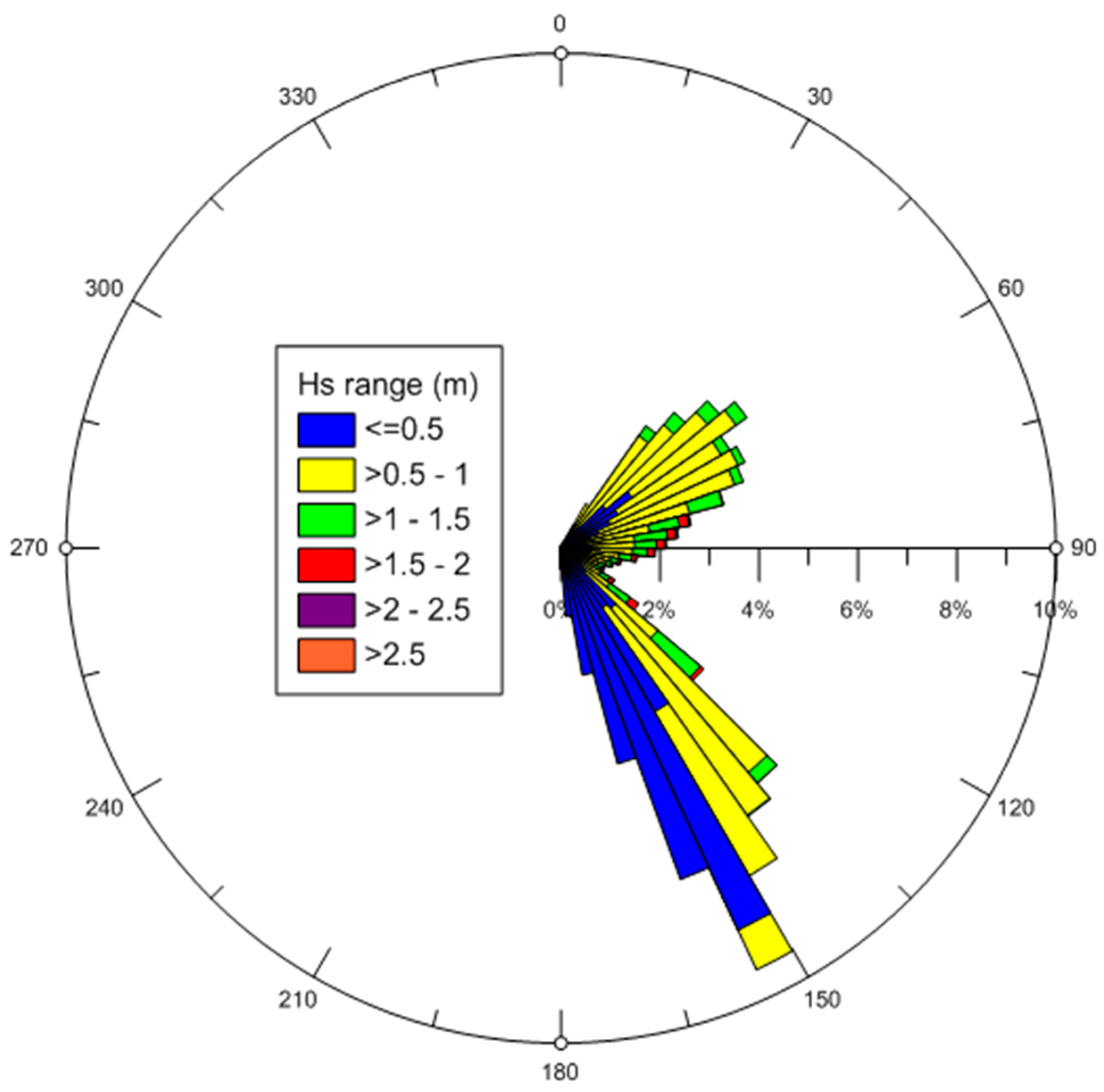
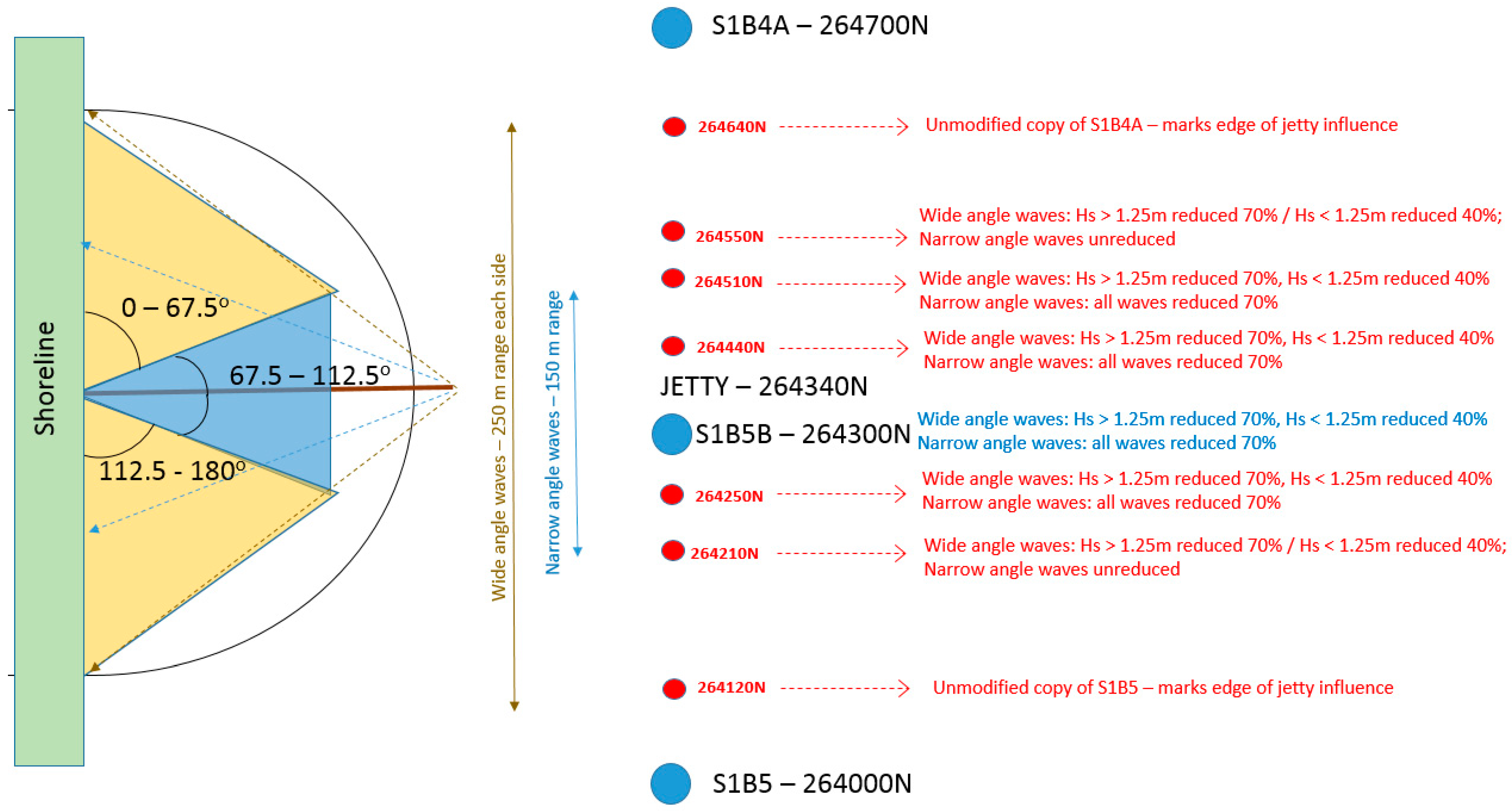
Inshore waves, already transformed by the nearshore banks and bars, are further refracted, diffracted and reflected by the structure.

(c)

The combined effect of tidal and wave orbital velocity act to re-suspend and advect sediments, taking account of gradients caused by the sheltering effect of the structure.

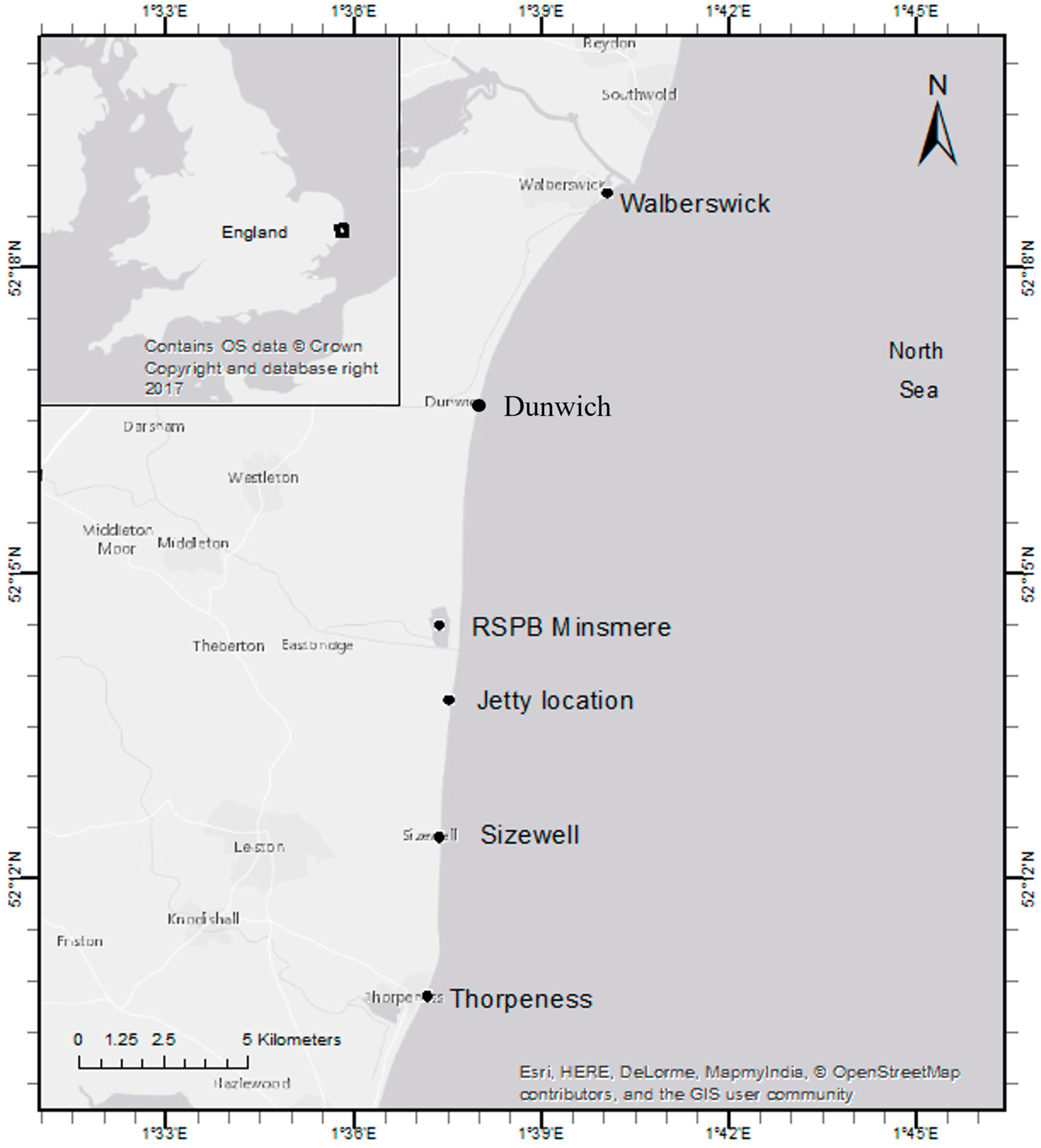
The method adopted used a TELEMAC2D (version v6p3) model to simulate the Sizewell tides (Section 2.2). Nearshore waves were generated by applying the offshore 33-year hindcast wave field (1980–2012), supplied by the Met Office European Wave Model, to the phase-averaging, spectral wave model, TOMAWAC (part of the open-source Telemac suite). TOMAWAC does not include the effects of diffraction or reflection. The resulting inshore wave data were used to define the specific wave case scenarios to run in ARTEMIS (Section 2.3), which does include these processes that are crucial to examining the impact of a structure such as a large jetty.

An external coupling between TELEMAC2D and ARTEMIS (Section 2.4) allowed the evaluation of the combined wave and current forces at the bed and the computation of nearshore bed shear stress, acting to move the sediment.

ARTEMIS was also externally coupled to the one-line UNIBEST model. Shoreline change modelling (Section 2.5) was driven with the whole wave climate and, to couple these models, it was necessary to derive, from the specific ARTEMIS scenarios, generalised rules for the changes imposed by the jetty in the properties of each wave condition in the hindcast (Section 2.6).

Figure 3 presents the schematic framework of the applied methodology.

2.1. Example Jetty

A typical proposed jetty is a large tubular piled structure with an overall length of approximately 640 m perpendicular to the shoreline. In keeping with many developments, this structure is assumed to be needed for 10 years whilst construction of shoreline structures occurs. Figure 4 shows the detail of the mesh at the jetty location and the layout of the piles, which are 1 m in diameter and 5 m apart.

For both TELEMAC2D and ARTEMIS model domains, the mesh was built in a parametric way where the triangles’ size and location could be specified using a script. Around the jetty, the mesh needed attributes to

• Simulate the rectilinear tidal currents between the shoreline and the end of the jetty.
• Replicate the structure of the jetty piles (diameter and spacing between piles) to a very fine resolution (20 cm). The fine mesh density around the piles is crucial to allow reflection and diffraction of waves from these features of the structure.
• Provide a resolution suitable to allow the TELEMAC2D model to be numerically stable and for waves to be resolved in length.
• Replicate the key bathymetric features over the domain (e.g., shore-parallel bars and the Sizewell Dunwich sandbank).

The scour predicted to be generated by the structure has been included in the bathymetry (referred to as AODN—Above Ordnance Datum Newlyn) prior to starting the simulations. Due to the high density of the piles, a global scour with a general deepening of the entire area is likely to occur—initially, a lowering of the bathymetry beneath the jetty in response to tidal current acceleration between the piles. Once volumetric continuity is re-established, flow and scour return to equilibrium. The depth of scour along the length of the jetty is unlikely to be homogeneous and is expected to be more extreme at the seaward end due to stronger tidal velocities.

2.2. TELEMAC2D Model

The hydrodynamic TELEMAC2D model [14] is used to simulate free surface flows in fluvial and coastal conditions and was used in this work to model the shore-parallel tidal currents. It solves depth-averaged, Saint-Venant shallow water equations, calculating the free surface, water depth and the two velocity components at each node of the irregular, finite-element triangular mesh.

The effect of the jetty piles on tidal currents was determined by running TELEMAC2D on an extremely fine mesh. This fine-scale model was nested in a regional scale tidal model, which used boundary conditions (velocities and sea level elevations) derived from observations made during an instrument deployment in November and December 2013. Velocity and elevation were extracted from the full regional tidal model at the appropriate locations of jetty tidal model boundaries and the jetty tidal model was run for 48 h for spring tide conditions.

The validation of the TELEMAC2D tidal model was performed using a harmonic analysis of individual time series of velocity components U and V and the free surface water elevation S, at the tidal model nodes coincident to observational lander positions. The six dominant harmonic components computed from modelled (Mod) and observed (Obs) values are compared at the inshore (IS) and offshore (OS) lander locations for the amplitude (m) and phase (deg) of the velocity components U and V and the free surface elevation S (

Table 1. Summary and comparison of major harmonic components.

	IS Velocity U					OS Velocity U
	Amplitude		Phase			Amplitude		Phase
	Obs	Mod	Obs	Mod		Obs	Mod	Obs	Mod
M2	0.098	0.040	27	27	M2	0.135	0.09	28	39
S2	0.018	0.007	70	79	S2	0.025	0.017	70	95
O1	0.004	0.004	321	272	O1	0.004	0.005	309	286
N2	0.018	0.008	20	341	N2	0.019	0.017	12	342
K1	0.005	0.001	81	63	K1	0.005	0.004	85	59
M4	0.008	0.005	355	4	M4	0.015	0.004	66	244
	IS Velocity V					OS Velocity V
	Amplitude		Phase			Amplitude		Phase
	Obs	Mod	Obs	Mod		Obs	Mod	Obs	Mod
M2	0.793	0.677	42	37	M2	0.809	0.744	41	39
S2	0.145	0.139	78	93	S2	0.154	0.15	85	95
O1	0.021	0.012	330	299	O1	0.024	0.022	333	296
N2	0.124	0.131	27	342	N2	0.118	0.144	25	342
K1	0.037	0.038	90	72	K1	0.032	0.029	100	101
M4	0.054	0.029	358	40	M4	0.049	0.02	33	44
	IS Elevation S					OS Elevation S
	Amplitude		Phase			Amplitude		Phase
	Obs	Mod	Obs	Mod		Obs	Mod	Obs	Mod
M2	0.784	0.721	290	295	M2	0.788	0.714	296	295
S2	0.152	0.115	322	357	S2	0.147	0.116	317	355
O1	0.115	0.147	181	171	O1	0.149	0.148	172	171
N2	0.119	0.141	280	324	N2	0.153	0.139	334	324
K1	0.155	0.128	323	320	K1	0.13	0.127	320	320
M4	0.056	0.08	359	349	M4	0.063	0.078	353	350

). The free surface elevations show an excellent comparison between the modelled and observed values, with a correlation around 0.98. The currents are rectilinear and dominated by the V component, which correlates with a coefficient above 0.95.

2.3. ARTEMIS Wave Model

The ARTEMIS wave module belongs to the Telemac modelling suite and performs the numerical simulation of wave propagation towards the coast or into harbours [15]. ARTEMIS has been used in a stand-alone mode, independently of other parts of the hydrodynamic system, and is used to compute the wave field only. This model has the capability of computing wave action where surface waves meet hard structures such as walls, breakwaters and coastal defence infrastructures. ARTEMIS includes parameters of reflection by an obstacle and diffraction behind an obstacle. These effects are combined with refraction due to bathymetric variation. ARTEMIS can be used to simulate multidirectional random waves; it includes non-linear effects of bottom friction and depth-induced breaking and reproduces associated energy dissipation for those two processes [15].

The wave boundary around the jetty has been designed as a semi-circle (diameter 2.7 km) to avoid corners and acute changes in the boundary angle and simplify boundary conditions. A very high-resolution mesh of 650,759 elements was used, with a resolution of 20 cm at the piles and 10 m at the ocean boundary. A constant initial tidal level (WL) was applied coincident with either the peak flood (from north to south) or ebb (from south to north) tide, and drying areas were not created, as the ARTEMIS model is unable to handle drying areas inside the domain. Taking into account TELEMAC2D results, a value of 0.30 m was used to coincide with the peak flood and −0.62 m for the peak ebb tide. Four significant wave heights (Hs) were considered (0.35, 1.0, 1.5 and 2.1 m). The multidirectional random waves option has been used as the input condition on the seaward boundary. The model simulates the directional spreading of the wave energy according to a pre-defined number of directions/periods and minimum and maximum angles of propagation/spectral period, where the angles are discretised into equal energy bands across the directional spread. ARTEMIS modelling is computationally resource-intensive and considers only a single wave case in each run. It was not possible to run each wave condition from the hindcast, so it was necessary to select specific wave cases from the nearshore hindcast climate, which would be representative of the impact of the jetty on the wave field.

To investigate the effect of the jetty on the waves coming from the two main sectors (Figure 2), wave directions (clockwise from north) of 75° and 157.5° were selected, with peak periods of 5.5 s (Hs = 0.35 and Hs = 1), 6 s (Hs = 1.5) and 7 s (Hs = 2.1). These wave directions were chosen to have both a low-obliquity (75°) and a high-obliquity (157.5°) scenario, accounting for all wave cases, as longshore sediment transport depends essentially on the wave obliquity with respect to the shoreline. It is expected that 157.5° waves will give a higher contribution for the longshore sediment transport. Waves from 75° are closer to being shore-normal, and the low angle of incidence to the shore suggests minimal longshore sediment transport driven by wave action. Simulations were performed for each combination of wave direction, wave height and tide peak (flood/ebb).

The ARTEMIS wave model is a steady-state simulation, and the results represent a snapshot in time and space of the computed wave field over the whole domain. This is based upon constant wave inputs at the boundaries as initial conditions.

Reflection Coefficient

ARTEMIS includes the effect of a solid boundary (such as the support piles of the jetty) when they reflect wave energy. The coefficient applied to evaluate this can vary between a value of 1 (perfect reflector—no absorption of wave energy) and a value of 0 (where all energy is absorbed at the solid boundary). A reflection coefficient of 1 at the pile boundaries would imply that no attenuation of the wave field occurs as they pass through the jetty. Conversely, with a reflection coefficient of 0, each contact of the wave with a pile boundary absorbs energy. It is crucial to use the most realistic value for this parameter, as it has a large impact on waves transmission, orbital currents and consequently on sediment transport and shoreline evolution.

There is little information in the literature regarding the values of reflection coefficients in pilled structures. Ref. [16] present several sensitivity tests to better understand the behaviour of the ARTEMIS model and its response to different types of structures and the imposed reflection coefficient. Taking into account the results obtained in that work and the few experimental observations available in the literature [17,18], these authors concluded that a reflection coefficient between 0.95 and 1.0 should be appropriate for piled structures with a pile spacing about 5 times the diameter, representing near-perfect reflection.

It is expected that the direct effect of the piles on waves at the Sizewell jetty will have less of an effect than the bathymetric changes under the jetty. Considering that piles in the real environment are unlikely to be perfect reflectors, the reflection coefficient used in this study was set to 0.95, resulting in the absorption of 5% of the wave energy by the piles.

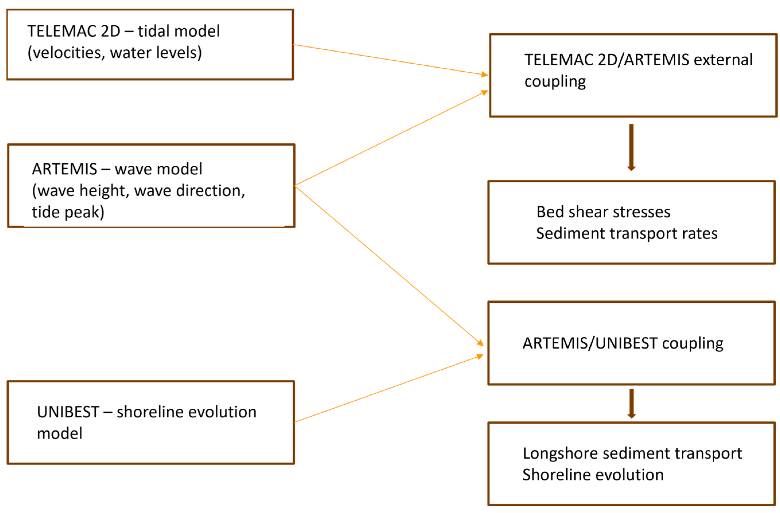
2.4. ARTEMIS/TELEMAC2D Coupling

An external coupling between ARTEMIS and TELEMAC2D was made in order to calculate the bed shear stresses and the sediment transport rates. This allows forcing from steady tidal currents and wave orbital velocities to be calculated separately, simulated by their respective models and combined as a post-processing operation. Ref. [19] synthesises the work carried out in the 1970s from many alternative research methods developed to determine non-linear enhancement to bed shear stress generated by wave/tide interaction. For this study, wave and tide velocity components were generated by the models and then combined by exporting tidal flow values at appropriate stages of the tide (peak flood and peak ebb) onto a 10 m regular grid over the jetty domain and combining with exported wave parameters over the same grid.

2.5. UNIBEST Model

The one-line shoreline model UNIBEST CL+ [10] was used in this study to determine shoreline evolution. The principles of one-line modelling are described in [20], and the performance of a range of models was reviewed by [21]. The UNIBEST model uses the angle between incident waves and the shoreline to calculate the longshore sediment transport due to the wave-induced component of current. Shoreline change (seaward or landward movement) is calculated from the gradients in the longshore transport rate and translated into a value for the advance or retreat of the shoreline. In one-line models, the cross-shore beach profile is fixed; shoreline change is simply a matter of lateral translations of this profile according to the volume of sediment gained or lost over time. The modelled shoreline is specified by a series of nodes. Input data (topographic profiles and hydrodynamic data) are specified at principal nodes and interpolated at intermediate nodes. Node spacing can vary—fewer nodes are required for straighter coastlines (associated with homogeneous forcing) or where longshore variation is low, while a higher concentration of nodes will be required to determine the local impact of structures.

The impact of the jetty was tested in a UNIBEST shoreline model covering 10 km of the Suffolk shoreline between Walberswick to the north of Sizewell and Thorpeness to the south (see Figure 1). Node spacing in this shoreline model was decreased around the jetty location specifically to capture the changes to nearshore waves revealed by the ARTEMIS modelling. At principal nodes, topographic profiles from the −5 m AODN elevation to the crest of the back-beach dune, at ca. 4–6 m AODN, were obtained from the Environment Agency.

In the modelled area, beaches above the mean water level largely consist of a thin veneer of fine to coarse gravel over a mixed sand–gravel sub-surface; below mean water, sampling only indicated predominantly sand-sized sediments. UNIBEST does not simulate a change in the cross-shore sediment distribution profile, and sediment transport formulae are available within the model only for sand- or gravel-sized sediments independently (and not mixed). Net transport of the beach gravel is thought to be minimal—the majority of sediment transport being of sub-tidal sand. Hence, a sand-only transport formulation was preferred and, of the available options within UNIBEST, the CROSMOR model described by [22,23] was selected for the following reasons:

• It offers the most complete description of the parameters influencing sediment transport [24];
• It contains sediment transport efficiency coefficients which parameterise conditions not otherwise captured by the model—such as rocky substrates and locally disrupted hydrodynamics around offshore structures.

UNIBEST model was calibrated by testing the model sensitivity to each of the potential input variables within reasonable ranges and selecting the variables that yielded, at the end of a 22-year model run, the closest match to observed net shoreline change observed at the major nodes.

UNIBEST was driven using the 22-year wave climate hindcast dataset shown in Figure 2 (for the period 1991–2012, to match available shoreline validation data), extracted at the 5 m depth contour at each of the principal UNIBEST nodes. Each annual wave climate is summarised with around 180 different combinations of wave height, period, direction and duration (as a fraction of the 365 days). UNIBEST propagates the waves from the 5 m contour to the shoreline, accounting for refraction, shoaling and dissipation (due wave breaking and bottom friction). Tides are not included.

2.6. ARTEMIS/UNIBEST Coupling

ARTEMIS modelling of the jetty considered four wave heights (0.35, 1.0, 1.5 and 2.1 m) and two main directions (75° and 157.5° wave angle) and water levels coincident with peak flood and ebb conditions (extracted from TELEMAC2D results). While the ARTEMIS model uses single wave cases forced along the semi-circular open boundary, UNIBEST uses annual wave climates, requiring point nodes and wave climate data at each point.

Waves approaching the jetty from the southeast or the northeast are attenuated by the jetty as energy is absorbed, reflected, dissipated and refracted. Figure 5 shows the location of the jetty and the attenuation of the waves in its lee, to the south with incident waves from 75° and to the north with waves from 157.5°, for ebb. Results are shown for ebb tide only as, for this condition, there is a higher impact from the jetty than for the flood. Figure 5 also represents the alongshore impact, which is about 150 and 250 m for the NE and SE waves, respectively.

The level of impact of the jetty on the wave scenarios included in the UNIBEST model is summarised in

Table 2. Wave height reduction, obtained by ARTEMIS model, for the various incident wave heights in two main directions.

75° (NE Waves)			157.5° (SE Waves)
Wave Height (m)	% Occurrence in Hindcast	% Reduction	Wave Height (m)	% Occurrence in Hindcast	% Reduction
0.35	56.5	60–80	0.35	84.8	40
1.0	37.6	60–80	1.0	13.1	40
1.5	4.7	70	1.5	1.75	60
2.1	1.2	80	2.1	0.35	70

. The jetty reduces wave heights on the downdrift side by 30–80%, with the largest waves being affected by larger reductions (Figure 5 and Table 2). This scale of impact is sufficient to affect shoreline evolution around the structure, as wave attenuation reduces re-suspension and longshore transport in the lee of the structure.

The percentage of occurrence presented in Table 2 was obtained based on Figure 2. The spatial extent of the jetty effect varies with the wave angle incidence such that with increasing obliquity between waves and the jetty (i.e., the SE wave case), the further alongshore the affected waves and impact of the jetty extend. However, these more oblique waves pass through fewer and more widely spaced piles and, for the lower wave heights, the impact of the jetty is reduced.

The ARTEMIS findings were condensed into four distinct rules or cases, which were applied to each wave in the full 22-year wave hindcast for UNIBEST modelling (see also Figure 6):

Narrow angle (<22.5° obliquity to the jetty) large (Hs > 1.25 m) wave case;

Narrow angle (<22.5° obliquity to the jetty) low (Hs < 1.25 m) wave case;

Wide angle (>22.5° obliquity to the jetty) large (Hs > 1.25 m) wave case;

Wide angle (>22.5° obliquity to the jetty) low (Hs < 1.25 m) wave case.

Although ARTEMIS modelling has included only wide angles from the SE direction and narrow angles from the NE, the results can be extrapolated to four cases, as the geometry of each wave angle is equivalent in each quadrant.

The impact of these rules on the applied wave climate in UNIBEST is summarised graphically in Figure 6. The physical structure of the jetty itself is not represented in the UNIBEST model (which does not contain any module suitable to represent a jetty or pier structure), i.e., it is not considered to be a physical barrier to the longshore sediment transport. The jetty impact is captured purely through the effect it has on the local nearshore waves, which ARTEMIS has shown to be limited to 250 m on each side of the structure. UNIBEST model node density is increased around the jetty location to capture effects at this scale.

Because UNIBEST interpolates between nodes, these should delineate the boundaries where behavioural change occurs within the model—thus, around the 150 m and 250 m limits of jetty impact, on the inside and outside edges of the envelopes for narrow-angle and wide-angle wave effects. This allows linear interpolation within each part of the envelope to be correct. The nodal system created for jetty modelling is shown in Figure 6.

2.7. Formulations

2.7.1. Bed Shear Stresses

The procedure used to calculate the bed shear stresses by [19] has been followed.

The mean (${\tau }_m$) and maximum (${\tau }_{max}$) bed shear stresses are defined in Equation (1) and Equation (2), respectively:

$${\tau }_m={\tau }_c\left[1+1.2{\left(\frac{{\tau }_w}{{\tau }_c+{\tau }_w}\right)}^{3.2}\right]$$

(1)

$${\tau }_{max}={\left[{\left({\tau }_m+{\tau }_w\cos \varnothing \right)}^2+{\left({\tau }_w\sin \varnothing \right)}^2\right]}^{\frac{1}{2}}$$

(2)

where ${\tau }_w$ is the wave-only bed shear stress, ${\tau }_c$ is the current-only bed shear stress and ∅ is the angle between current direction and direction of wave travel. The north–south orientation of the site allowed an assumption that tidal currents are running north/south, and values of 0° and 180° were used for the currents. While ${\tau }_m$ is used for determining the sediment diffusion into the outer flow, ${\tau }_{max}$ is used to determine whether the threshold of sediment motion has been exceeded and for near-bed diffusion.

The current-only bed shear stress (${\tau }_c$) is evaluated by

$${\tau }_c={\rho }_w{C}_D{\overline{U}}^2$$

(3)

where ${\rho }_w$ is the water density, which was assumed to be 1027 kg/m³; $C_D$ is the drag coefficient of a steady current in the absence of waves, considered to be 0.00458 [19]; and $\overline{U}$ is the depth-averaged current velocity.

The wave-only bed shear stress (${\tau }_w$) was calculated using Equation (4):

$${\tau }_w=\frac{1}{2}{\rho }_w{f}_w{U_w}^2$$

(4)

where $U_w$ is the near-bed orbital velocity amplitude (Equation (8)) and $f_w$ is the wave friction factor calculated by Equation (5):

$$f_w=max\left(f_{wr}, f_{ws}\right)$$

(5)

where $f_{wr}$ is the rough-bed friction factor (Equation (6)) and $f_{ws}$ is the smooth-bed friction factor (Equation (9)):

$$f_{wr}=1.39{\left(\frac{A}{z_0}\right)}^{-0.52}$$

(6)

where $z_0$ is the roughness length, assumed to be 6 mm, and A is the orbital amplitude of wave motion at the bed (Equation (7)):

$$A=\frac{U_w{T}_p}{2\pi }$$

(7)

where $T_p$ is the peak wave period and $U_w$ is given by (Equation (8)):

$$U_w=\sqrt{2} U_{rms}$$

(8)

where $U_{rms}$ is the root-mean-square wave orbital velocity.

$$f_{ws}=B{R_w}^{-N}$$

(9)

where

$$\begin{gathered} B=2,\hspace{1em}N=0.5\hspace{1em}\mathrm{for}\hspace{1em}{R}_w\le 5\times {10}^5 \\ B=0.0521,\hspace{1em}N=0.187\hspace{1em}\mathrm{for}\hspace{1em}{R}_w>5\times {10}^5 \end{gathered}$$

and $R_w$ is the wave Reynolds number:

$$R_w=\frac{U_{w}A}{\nu }$$

(10)

with a kinematic viscosity of water ($\nu$) of 1.36 × 10⁻⁶ m²/s.

The root-mean-square wave orbital velocity ($U_{rms}$) is calculated through Equation (11) [25]:

$$U_{rms}=\left(\frac{H_s}{4}\right){\left(\frac{g}{h}\right)}^{\frac{1}{2}}\exp \left\{-{\left[\frac{3.65}{T_z}{\left(\frac{h}{g}\right)}^{\frac{1}{2}}\right]}^{2.1}\right\}$$

(11)

where $H_s$ is the significant wave height, $h$ is the still water depth, $g$ is the acceleration due to gravity and $T_z$ is the zero up-crossing wave period, which is empirically computed in this case as $T_z=0.781T_p$.

2.7.2. Sediment Transport Rates

The total sediment transport rate ($q_t$) by waves plus currents was computed using the formulation of Soulsby–Van Rijn [19]:

$$q_t=A_s\overline{U}{\left[{\left({\overline{U}}^2+\frac{0.018}{C_D}{U}_{rms}^2\right)}^{1/2}-{\overline{U}}_{cr}\right]}^{2.4}\left(1-1.6\tan \beta \right)$$

(12)

where ${\overline{U}}_{cr}$ is the threshold current velocity and $\beta$ corresponds to the slope of the bed in the streamwise direction. It was assumed to be a flat sea bed ($\beta$ = 0).

$$A_s=A_{sb}+A_{ss}$$

(13)

corresponding $A_{sb}$ to bedload and $A_{ss}$ to suspended load transport:

$$A_{sb}=\frac{0.005h{\left(d_{50}/h\right)}^{1.2}}{{\left[\left(s-1\right)g{d}_{50}\right]}^{1.2}}$$

(14)

$$A_{ss}=\frac{0.012d_{50}{D}_{*}^{-0.6}}{{\left[\left(s-1\right)g{d}_{50}\right]}^{1.2}}$$

(15)

where $d_{50}$ is the median diameter of sediment grains (350 µm), s is the ratio of density of sand to water assuming the grain density is the same as quartz grain (2650 kg/m³) and $D_{*}$ is the dimensionless grain size:

$$D_{*}={\left[\frac{g\left(s-1\right)}{{\nu }^2}\right]}^{\frac{1}{3}}{d}_{50}$$

(16)

The threshold current velocity ${\overline{U}}_{cr}$ is calculated using Equation (17):

$${\overline{U}}_{cr}=7{\left(\frac{h}{d_{50}}\right)}^{1/7}{\left[g\left(s-1\right)d_{50}f\left(D_{*}\right)\right]}^{1/2} for D_{*}>0.1$$

(17)

where

$$f\left(D_{*}\right)=\frac{0.30}{1+1.2D_{*}}+0.055\left[1-\exp \left(-0.020D_{*}\right)\right]$$

(18)

The vector quantity of sediment transport rate (${\mathit{q}}_{\mathit{t}}$) can be written as [19]

$${\mathit{q}}_{\mathit{t}}=\left(q_{tx},q_{ty}\right)=\left(\left|{\mathit{q}}_{\mathit{t}}\right|\frac{U_x}{\left|\mathit{U}\right|}, \left|{\mathit{q}}_{\mathit{t}}\right|\frac{U_y}{\left|\mathit{U}\right|}\right)$$

(19)

where

$q_{tx},q_{ty}$ = components of sediment transport rate in x and y directions;

$\mathit{U}$ = $\left(U_x,U_y\right)$ = current velocity vector;

$U_x,U_y$ = components of current velocity in x and y directions;

$\left|{\mathit{q}}_{\mathit{t}}\right|$, $\left|\mathit{U}\right|$ = magnitudes of sediment transport rate and current speed.

The direction of sediment flux was determined by the conversion of the sediment transport rates to vectors. The component of sediment transport in x ($q_{tx}$) and y ($q_{ty}$) directions are given by

$$q_{tx}=\left|{\mathit{q}}_{\mathit{t}}\right|\frac{U_x}{\sqrt{U_x^2+U_y^2}}$$

(20)

$$q_{ty}=\left|{\mathit{q}}_{\mathit{t}}\right|\frac{U_y}{\sqrt{U_x^2+U_y^2}}$$

(21)

2.7.3. Threshold Bed Shear Stress

The threshold value of the bed shear stress is one of the most important factors when determining bed or suspended sediment response to hydrodynamic flow. The critical conditions for sediment entrainment were determined following [19].

The critical bed shear stress ${\tau }_{cr}$ depends on the physical properties of sediment and water only and is obtained using the threshold Shields parameter $f\left(D_{*}\right)$ (Equation (18)) and the dimensionless grain size (Equation (16)):

$${\tau }_{cr}=f\left(D_{*}\right)g\left({\rho }_s-{\rho }_w\right)d_{50}$$

(22)

where ${\rho }_s$ is the grain density.

3. Results and Discussion

The bed shear stresses, shoreline evolution and sediment transport rates are shown and discussed in this section.

The threshold value of the bed shear stress is one of the most important factors when determining bed or suspended sediment response to hydrodynamic flow. As the velocity of the fluid flow over a sand bed increases, there is a stage when the stress exerted by the fluid on the particles is enough to cause them to move into the flow. The threshold of sediment movement is fundamental when evaluating the sediment response to currents or waves. Using Equation (22), a threshold bed shear stress of 0.216 N/m² was obtained. Therefore, a direct comparison between the bed shear stress generated by hydrodynamic forcing and the value at which sediment mobility is expected to occur can be made.

3.1. Bed Shear Stress

For the dominant and commonly occurring wave height of 0.35 m, while there is a significant height attenuation (due to the jetty), these waves have little effect on sediment transport and impart little or no bed shear stress until they reach the coast. Previous work on the East Anglian coasts, in sediment of a slightly finer nature than at Sizewell, has shown that only waves over 1 m have a significant effect on sediment transport and that waves of less than 0.5 m only act to stir sediment [26].

Table 3. (a) Bed shear stress calculations made at the point shown in the lee of the jetty for waves from 157.5°. (b) Bed shear stress calculations made at the point shown in the lee of the jetty, for waves from 75°.

(a)
	Boundary Condition: 157.5°, $H_s$ = 1.5 m
	WL= 0.30 m (Flood)		WL = −0.62 m (Ebb)
	Jetty	No-Jetty	Jetty	No-Jetty
$H_s$ (m)	0.54	1.11	0.33	0.96
$h$ (m)	4.11	4.11	3.19	3.19
$\overline{U}$ (m/s)	0.39	0.38	0.44	0.42
$U_w$ (m/s)	0.23	0.48	0.17	0.50
${\tau }_c$ (N/m2)	0.71	0.69	0.91	0.83
${\tau }_w$ (N/m2)	5.85	17.03	3.80	18.22
${\tau }_m$ (N/m2)	1.30	1.41	1.46	1.70
${\tau }_{max}$ (N/m2)	4.67	15.74	5.17	19.80
(b)
	Boundary Condition: 75°, $H_s$ = 1.5 m
	WL = 0.30 m (Flood)		WL = −0.62 m (Ebb)
	Jetty	No-Jetty	Jetty	No-Jetty
$H_s$ (m)	0.13	1.42	0.12	1.32
$h$ (m)	4.66	4.66	3.74	3.74
$\overline{U}$ (m/s)	0.46	0.44	0.49	0.49
$U_w$ (m/s)	0.05	0.56	0.06	0.61
${\tau }_c$ (N/m2)	0.99	0.93	1.15	1.14
${\tau }_w$ (N/m2)	0.60	21.49	0.72	24.44
${\tau }_m$ (N/m2)	1.04	1.90	1.21	2.33
${\tau }_{max}$ (N/m2)	1.33	22.06	1.24	23.94

a,b present the bed shear stresses, calculated at a point in the lee of the jetty (represented as a star symbol in Figure 5) where waves are strongly attenuated, for 1.5 m waves coming from 157.5° and 75°, respectively. The calculations are made for both ebb and flood tides and for the situations considering or not considering the presence of the jetty.

Both Table 3a,b show very little difference between the wave attenuation observed during an ebb or a flood tide, as depth is the only factor changed in the calculation between phases of the tide. The bed shear stress due to the tidal currents is also similar in these locations. A much more significant reduction is seen in the bed shear stress generated by wave orbital currents (${\tau }_w$) and the enhanced value of maximum shear stress (${\tau }_{max}$), where values are 30% of their original value during the flood and only 26% during the ebb for 157.5° waves. For 75° waves, the maximum shear stress values are 6% of the original for flood and 5% for ebb.

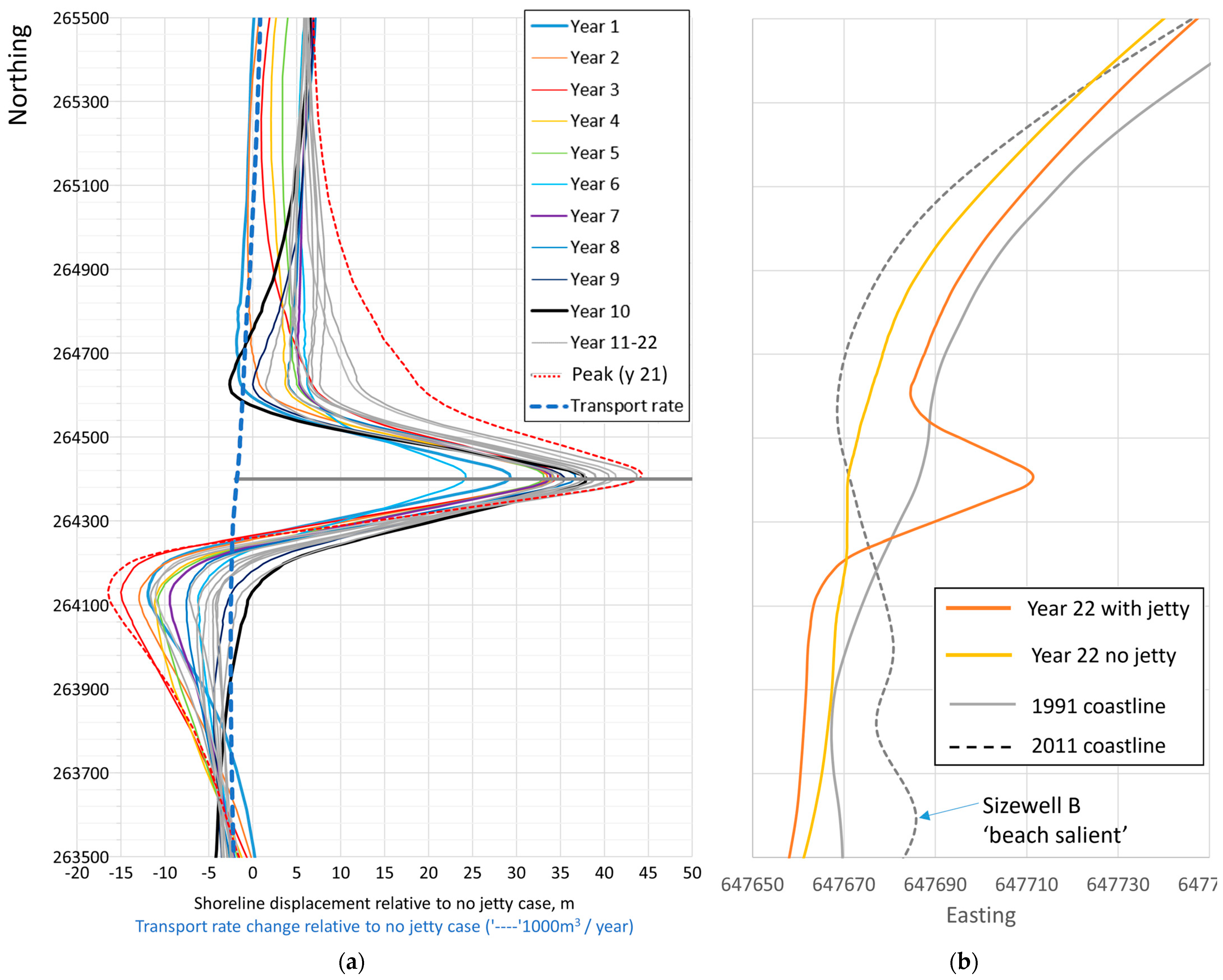
3.2. Shoreline Evolution

The UNIBEST models using the 22-year wave hindcast data both with and without the jetty each generate year-by-year estimates of shoreline position. The non-jetty case gives an estimate of the natural envelope of change (the shoreline at any given position moving back and forth according to the net balance of sediment transport due to the waves in any given year). Shoreline change in the UNIBEST model is not monotonic with time: the shoreline may advance or retreat by up to 5 m each year, depending on the changing directional bias of the net annual wave climate.

The maximum year-on-year difference in shoreline positions between the model runs with the jetty and without is 45 m and occurs at the site of the jetty. The distance at which displacement of the shoreline (relative to the non-jetty case) is greater than the natural shoreline variability envelope is within 500–800 m north or south of the jetty itself (Figure 7). Figure 7a suggests that the impacts from the jetty on net longshore sediment transport rates and shoreline evolution are largely confined within the range of the wave impacts derived from ARTEMIS. The region of influence of the jetty is very similar to that obtained by [8] for the jetty at Duck, North Carolina.

Net sediment transport within the zone affected by the jetty is southward, at low net rates and with very little longshore gradient. As a result, there is a comparable scale of impact on each side of the jetty with just a slight asymmetry due to the low net southward bias in transport and the slight difference in the original orientation of the shorelines north and south of the jetty location. This results in a net stable shoreline south of the field of influence of the jetty.

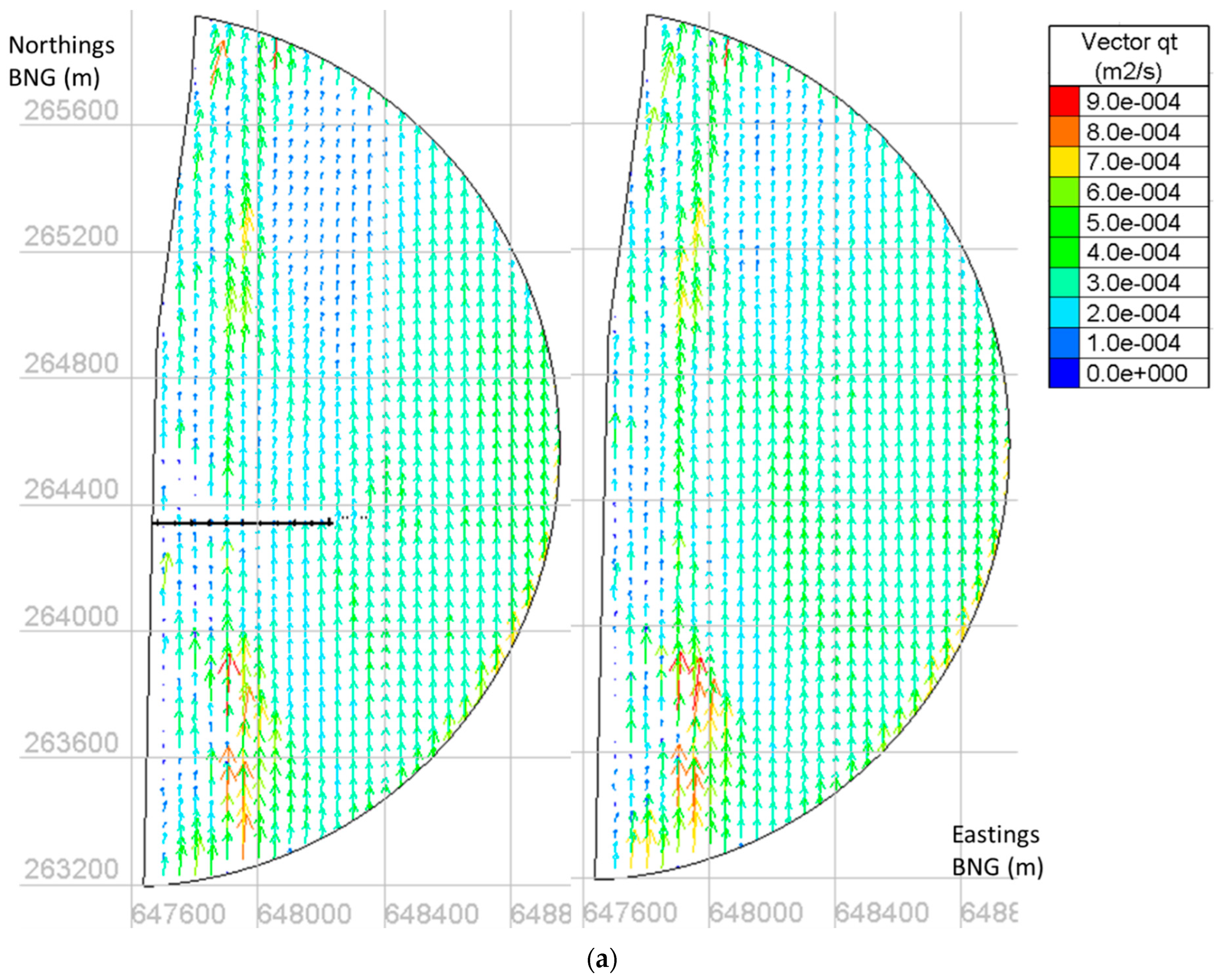
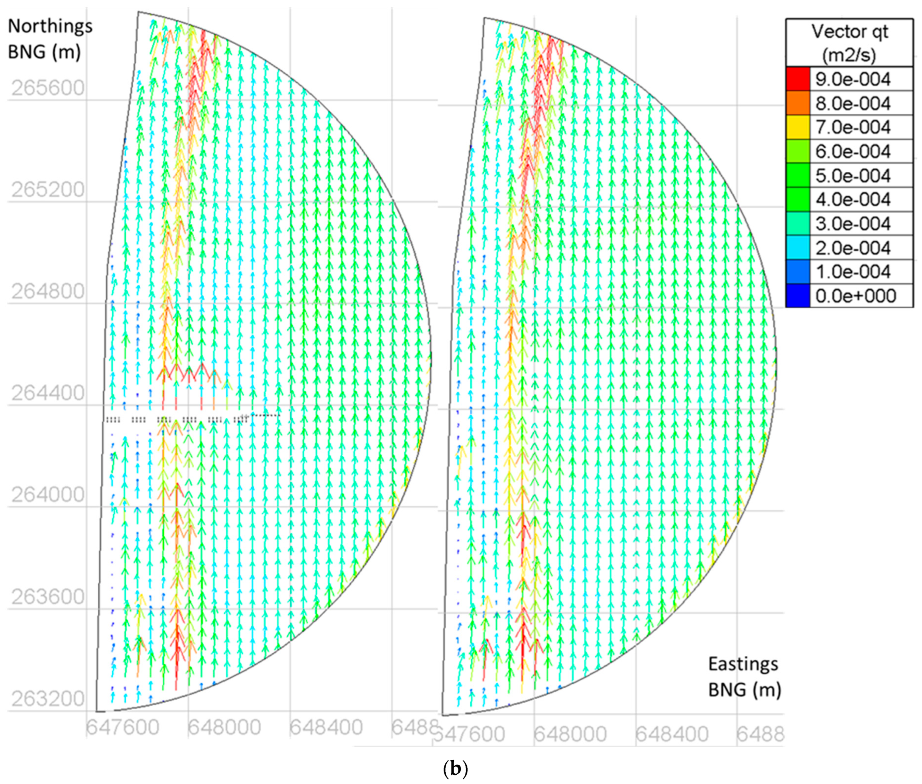
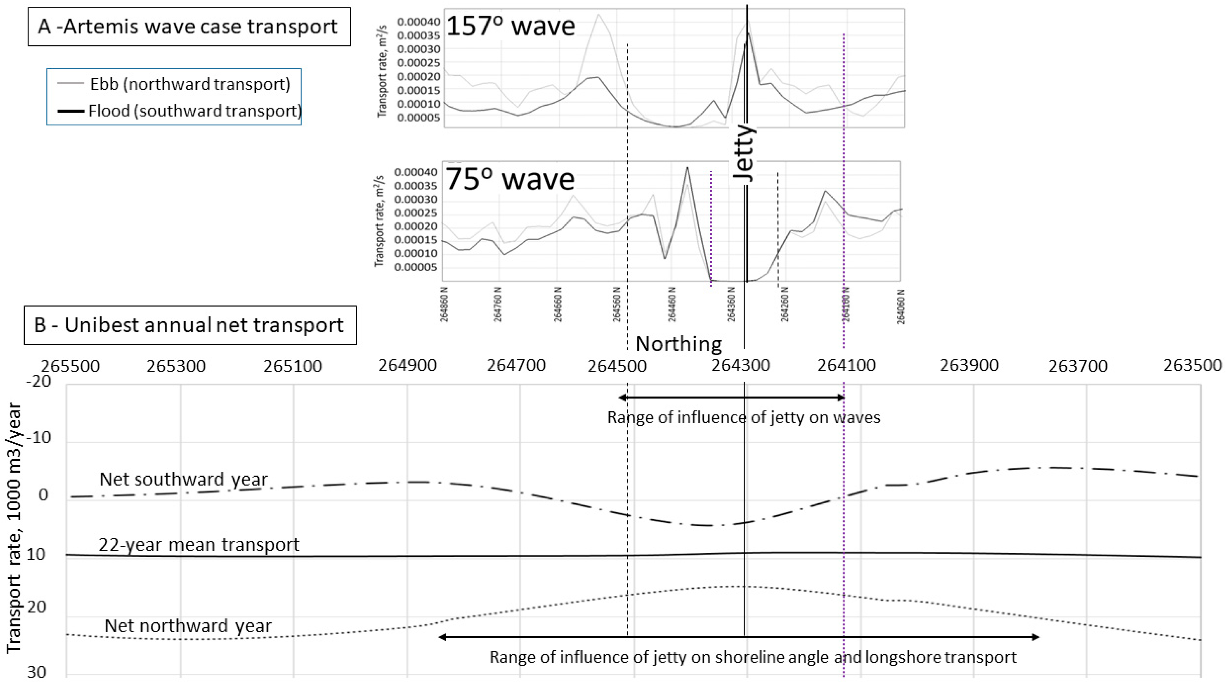
3.3. Sediment Transport Rates

Both the ARTEMIS and the UNIBEST models produce sediment transport rate estimates for the impact of the proposed jetty, the former for single wave cases over a tidal cycle and the latter as a net yearly longshore transport. Whereas using ARTEMIS/TELEMAC2D, the transport is calculated on a purely physical hydrodynamic basis, longshore transport in UNIBEST is affected by an additional geographical component: the shoreline orientation.

Figure 8 presents the total (wave and tide) sediment transport rates for ARTEMIS. The tidal currents (particularly on springs) are strong, and therefore, tidal currents coupled with waves of 2.1 m are considered for total load sediment transport analysis. Figure 8 shows the vector quantity of sediment transport rate for ebb with and without the jetty, for both waves from 157.5° and 75°. The size of the vectors represents their magnitude. The observed higher sediment transport rates in a shore-parallel orientation, at about 300 m offshore, is coincident with the location of an existing longshore sand bar (so supporting the selection of the sand transport model in UNIBEST—which also generates an offshore transport peak).

For waves coming from 157.5°, a zone of low sediment transport is apparent in the shallow waters, north of the jetty, because of the wave shadow it creates for the southeast waves. At this location, the transport rates are low because of the reduction in suspended sediment due to lower wave-induced bed shear stress. This behaviour would cause, for these shallow waters, deposition under the jetty for ebb and erosion for floods.

For waves from 75°, a zone of low sediment transport is also observed in shallow waters in the wave shadow, now south of the jetty. In this case, there will be erosion under the jetty for ebb and deposition for flood.

The sediment transport rate on a transect inshore of the longshore bar in the ARTEMIS wave cases (Figure 9) is almost tidally symmetrical; i.e., ebb (northward) and flood (southward) transport rates are similar, indicating a low net transport. However, calculated transport drops to almost zero in the wave shadow of the jetty, indicating net sediment convergence at this location. Sediment convergence would suggest shoreline accretion at this location, on both sides of the jetty, matching the result obtained in UNIBEST (Figure 7).

UNIBEST results suggest that the long-term mean longshore transport rate past the jetty is largely unaffected by the jetty; i.e., mean sediment transport over the whole 22-year period is almost identical between runs. However, the jetty reduces the year-by-year variation in transport rate (Figure 9). The change in shoreline orientation around the jetty increases the angle between the wave and the shore, which compensates for the reduction in overall wave energy due to the jetty. The change in angle causes the longshore transport rate to decrease on the updrift side of the jetty and increase on the downdrift side—leading to the ‘hourglass’ effect shown in Figure 9. The impact on longshore transport extends over a wider area than the effects indicated by the ARTEMIS wave modelling.

Both the longshore and cross-shore extent of the shoreline change due to the jetty predicted by the modelling is very similar to the actual shoreline perturbation known as the ‘beach salient’ (marked on Figure 7b), which is purportedly associated with the presence of a cooling water outfall at Sizewell B power station. The longshore bars deviate around the outfall, and there is a considerable scour pit around it, which, like the hypothetical jetty, may have a local effect on incident wave climate. Within UNIBEST, the size of the predicted shoreline perturbation is proportional to the mean longshore transport gradient past the structure, and this is comparably low at both the jetty and outfall locations.

The average longshore transport in the model domain, over the period 1991–2012, is in agreement with previous modelled estimates: being net southward and declining from Dunwich towards Thorpeness. Rates agree with the lower limits reported by [27] (11,000 m³ p.a. north of Dunwich and 3450 m³ p.a. at Sizewell) and similar modelling undertaken by [28] (see Figure 10). Figure 10 shows the mean transport rate at different locations along the coastline, for sand, gravel and shingle. A comparison of the net longshore transport rate obtained by different authors is presented in

Table 4. Net longshore transport rate along the coastline obtained by different authors.

Author	Site	Net Transport Rate (m3/Year)
Vincent (1979) [29]	Dunwich	70,000
Onyett and Simmonds (1983) [30]	Southwold	200,000
	Walberswick	210,000
	Dunwich Thorpeness North Thorpeness South	130,000 200,000 55,000
Halcrow (2001) [31]	Southwold	3100
	Corporation Marsh	9900
	Dunwich Minsmere sluice Sizewell Power Station Thorpeness	12,100 3200 3700 300
Black and Veatch (2005) [28]	Dunwich cliffs	13,000
	S1B2	19,700
	S1B4 S1B4 (offshore) S1B6 Ness House (~S1B7)	8100 (northward) 8900 9300 2200 (northward)

.

It should be noted that the UNIBEST model does not account for the increased current speeds which would result from the constriction of tidal flow under the structure. This would tend to promote scour and discourage deposition, which could to some extent compensate for the effect of the reduction in wave heights. Furthermore, there are limitations associated with the one-line shoreline modelling technique, e.g., no capacity to account for cross-shore change. The hindcast applied to UNIBEST was (of necessity) derived from a limited number of modelled wave cases, each of which in turn is based on further limiting assumptions. It is not possible for the wave hindcast to represent the full range of wave heights, periods and directions experienced at the Sizewell shoreline over a 22-year period.

Therefore, this modelling process should not be expected to accurately reproduce all the details of shoreline variability. Likewise, modelled outcomes are not predictions of future shorelines but should be treated as indicative estimates of the scale and likely general impact of shoreline interventions. Nevertheless, the applied methodology proves to be efficient and allows the influence of the jetty on waves, as determined by the ARTEMIS model, to be represented within the UNIBEST model even though the latter does not allow the physical representation of the jetty.

4. Conclusions

This work presents a new methodology to determine the likely effects of a jetty on longshore dynamics and shoreline evolution at Sizewell Bay. This methodology involves the application of ARTEMIS wave model, the TELEMAC2D tidal model and the UNIBEST shoreline evolution model, along with their external coupling. The effect of the jetty on nearshore wave climate was assessed considering wave action alone, as sediment re-suspension during high energy wave events is the dominant mode of longshore transport, and considering combined waves and currents to generate an enhanced bed shear stress. The information on the waves’ transformation by the structure, obtained from ARTEMIS, was then used to define the wave heights in the UNIBEST model. This methodology, apart from the possibility of being applied worldwide, can easily account for climate change conditions, including different wave climate scenarios.

The wave model has shown that the jetty will alter the alongshore wave-energy distribution up to about 500 m alongshore. The UNIBEST shoreline modelling results with the jetty suggest that the shoreline will be displaced seaward by up to 45 m at the jetty location. Immediately south of the jetty, the model suggests a much smaller landward retreat (e.g., by about 15 m at a location 200 m south of the jetty) compared with the no-jetty case. The cross-shore and longshore scale of influence is similar to an observed shoreline perturbation at Sizewell B, which may be due to similar localised changes in incident waves and is also similar to observed changes around the jetty at Duck, North Carolina. Furthermore, the predicted longshore transport rates along the coastline are in agreement with findings from previous studies. This implies that the applied methodology can provide reliable results in predicting the impact of a marine structure on shoreline evolution.

References

1. Linley, E.A.S.; Wilding, T.A.; Black, K.D.; Hawkins, A.J.S.; Mangi, S. Review of the reef effects of offshore wind farm structures and potential for enhancement and mitigation. Peer-Rev. Rep. 2008, 132, 1. [Google Scholar]
2. Lindeboom, H.J.; Kouwenhoven, H.J.; Bergman, M.J.N.; Bouma, S.; Brasseur, S.; Daan, R.; Fijn, R.C.; de Haan, D.; Dirksen, S.; van Hal, R.; et al. Short-term ecological effects of an offshore wind farm in the Dutch coastal zone; a compilation. Environ. Res. Lett. 2011, 6, 35101. [Google Scholar] [CrossRef]
3. Brown, J.M.; Morrissey, K.; Knight, P.; Prime, T.D.; Almeida, L.P.; Masselink, G.; Bird, C.O.; Dodds, D.; Plater, A.J. A coastal vulnerability assessment for planning climate resilient infrastructure. Ocean Coast. Manag. 2018, 163, 101–112. [Google Scholar] [CrossRef]
4. Jones, P.J.S. Fishing industry and related perspectives on the issues raised by no-take marine protected area proposals. Mar. Policy 2008, 32, 749–758. [Google Scholar] [CrossRef]
5. Gleason, M.; Fox, E.; Ashcraft, S.; Vasques, J.; Whiteman, E.; Serpa, P.; Saarman, E.; Caldwell, M.; Frimodig, A.; Miller-Henson, M.; et al. Designing a network of marine protected areas in California: Achievements, costs, lessons learned, and challenges ahead. Ocean. Coast. Manag. 2013, 74, 90–101. [Google Scholar] [CrossRef]
6. Whitehouse, R.; Harris, J.; Sutherland, J. Marine Scour Course; HR Wallingford, Howbery Park: Wallingford, UK, 2012. [Google Scholar]
7. Garel, E.; Sousa, C.; Ferreira, O. Sand bypass and updrift beach evolution after jetty construction at an ebb-tidal delta. Estuar. Coast. Shelf Sci. 2015, 167, 4–13. [Google Scholar] [CrossRef]
8. Pianca, C.; Holman, R.; Siegle, E. Shoreline variability from days to decades: Results of long-term video imaging. J. Geophys. Res. Oceans 2015, 120, 2159–2178. [Google Scholar] [CrossRef]
9. Beraud, C.; Wallbridge, S. Assessing long-term effect of a Beach Landing Facility on a soft evolving coast using UNIBEST model. In Proceedings of the RCEM congress (River Coastal and Estuarine Morphodynamics), Iquitos, Peru, 30 August–3 September 2015. [Google Scholar]
10. Deltares. UNIBEST CL+. Available online: https://www.deltares.nl/en/software/UNIBEST-cl/#8 (accessed on 22 May 2015).
11. Araújo, M.A.V.C.; Di Bona, S.; Trigo-Teixeira, A. Impact of detached breakwaters on shoreline evolution: A case study on the Portuguese west coast. In Proceedings of the 13th International Coastal Symposium, Durban, South Africa, 13–17 April 2014; Green, A.N., Cooper, J.A.G., Eds.; pp. 41–46. [Google Scholar]
12. Thiruvenkatasamy, K.; Baby Girija, D.K. Shoreline evolution due to construction of rubble mound jetties at Munambam inlet in ErnakulameTrichur district of the state of Kerala in the Indian peninsula. Ocean Coast. Manag. 2014, 102, 234–247. [Google Scholar] [CrossRef]
13. Bacon, J.C.; Vincent, C.E.; Dolphin, T.J.; Taylor, J.A.; Pan, S.-Q.; O’Connor, B.A. Shore-parallel breakwaters in meso-tidal conditions: Tidal controls on sediment transport and their longer term, regional impacts at Sea Palling, UK. In Proceedings of the 9th International Coastal Symposium, Gold Coast, Australia, 16–20 April 2007; pp. 369–373. [Google Scholar]
14. EDF R&D. TELEMAC Modelling System, 2D Hydrodynamics TELEMAC2D Software Version 7.0 User Manual; EDF R&D: Paris, France, 2014. [Google Scholar]
15. EDF R&D. The TELEMAC Modelling System, Theoretical Note and User Manual—ARTEMIS Software for Wave Agitation, Version 6.2; EDF R&D: Paris, France, 2012. [Google Scholar]
16. Araujo, M.A.; Fernand, L.; Bacon, J. Sensitivity analysis to reflection and diffraction in ARTEMIS. In Proceedings of the XXVth TELEMAC-MASCARET User Conference, Norwich, UK, 9–11 October 2018. [Google Scholar]
17. Truitt, C.L.; Herbich, J.B. Transmission of random waves through pile breakwaters. In Coastal Engineering 1986; ASCE: New York, NY, USA, 1986; Chapter 169. [Google Scholar]
18. Van Weele, B. Wave Reflection and Transmission for Cylindrical Pile Arrays; May 1965, Reprint no 313. Fritz Laboratory Reports, Paper 183. Master’s Thesis, Lehigh University, Bethlehem, PA, USA, 1965. [Google Scholar]
19. Soulsby, R.L. Dynamics of Marine Sands; Thomas Telford: London, UK, 1997. [Google Scholar]
20. Hanson, H.; Arrninkhof, S.; Capobianco, M.; Mimenez, J.A.; Karson, M.; Nicholls, R.J.; Plant, N.G.; Southgate, H.N.; Steetzel, H.J.; Stive, M.J.F.; et al. Modelling of coastal evolution on early and decadal time scales. J. Coast. Res. 2003, 19, 790–811. [Google Scholar]
21. Thomas, R.C.; Frey, A.E. Shoreline Change Modeling Using One-Line Models: General Model Comparison and Literature Review; ERDC/CHL CHETN-II-55; US Army Engineer Research and Development Center: Vicksburg, MS, USA, 2013; 9p. [Google Scholar]
22. Van Rijn, L.C. Principles of Sediment Transport in Rivers, Estuaries and Coastal Seas Part 1; Aqua Publications: Amsterdam, The Netherlands, 1993. [Google Scholar]
23. Van Rijn, L.C. Principles of Sediment Transport in Rivers, Estuaries and Coastal Seas Part 2 (Supplement); Aqua Publications: Amsterdam, The Netherlands, 2006. [Google Scholar]
24. Mil-Homens, J.; Ranasinghe, R.; van Thiel de Vries, J.S.M.; Stive, M. Influence of profile features on longshore sediment transport. In Proceedings of the Coastal Dynamics 2013: 7th International Conference on Coastal Dynamics, Arcachon, France, 24–28 June 2013; Volume 13, pp. 1219–1228. [Google Scholar]
25. Soulsby, R.L. Simplified Calculation of Wave Orbital Velocities; Report TR 155, Release 1.0; HR Wallingford: Oxfordshire, UK, 2006. [Google Scholar]
26. Bacon, J.C. The Shore-Parallel Breakwaters at Sea Palling: Interaction with Tidal Currents and Their Contribution to Sediment Transport. Ph.D. Thesis, University of East Anglia, Norwich, UK, 2005. [Google Scholar]
27. HR Wallingford; CEFAS/UEA; Posford Haskoning; D’Olier, B. Southern North Sea sediment Transport Study, Phase 2: Sediment Transport Report; Report EX 4526; Appendix 11: Report on Southern North Sea longshore sediment transport; HR Wallingford: Oxfordshire, UK, 2002; 146p. [Google Scholar]
28. Black and Veatch. Minsmere Frontage: Dunwich Cliffs to Sizewell Power Stations, Coastal Processes Report; Environment Agency: Bristol, UK, 2005. [Google Scholar]
29. Vincent, C.E. Longshore sand transport rates—A simple model for the East Anglian coastline. Coast. Eng. 1979, 3, 113–136. [Google Scholar] [CrossRef]
30. Onyett, D.; Simmonds, A. East Anglian Coastal Research Programme Final Report 8: Beach Transport and Longshore Transport; GeoBooks: Norwick, UK, 1983. [Google Scholar]
31. Halcrow Group Ltd. Lowestoft to Thorpeness Coastal Process and Strategy Study Volume 2: Coastal Processes; Halcrow Inc.: New York, NY, USA, 2001. [Google Scholar]
Figure 1. Study area from Walberswick to Thorpeness, including RSPB Minsmere and jetty locations.
Water 16 00705 g001
Figure 2. Model derived inshore waves at Sizewell for the period 1991–2012.
Water 16 00705 g002
Figure 3. Schematic framework of the applied methodology.
Water 16 00705 g003
Figure 4. Mesh design and incorporation of pile detail.
Water 16 00705 g004
Figure 5. Wave height reduction (ebb): (a) NE waves (75°) are reduced 60–80% across all wave heights; (b) SE wave (157.5°) reduction varies with wave height, with only the larger waves (>1.5 m) being reduced by 80% and the jetty having less impact on smaller waves. The jetty is represented with marked black lines.
Water 16 00705 g005
Figure 6. Summary of the impact of the jetty on waves. The schematic graphic (left) shows the sectors which define waves as wide- or narrow-angle, with arrows indicating the approach of waves past the jetty and marking zones of influence of the jetty on the shoreline. Since only one principal UNIBEST node (right) is within this zone of influence, secondary nodes (small circles) have been created at the locations shown, by amending the wide and narrow waves according to the ARTEMIS modelling outcomes.
Water 16 00705 g006
Figure 7. (a) Difference in shoreline displacement between the UNIBEST runs with and without the jetty (with negative values indicating a more landward shoreline with the jetty and positive indicating a more seaward shoreline). Each line represents the displacement in each year of the 22-year wave hindcast. The dashed blue line represents the change in mean sediment transport rate from the baseline when the jetty is added. (b) Predicted and measured shorelines, showing a 20–30 m shoreline perturbation due to the jetty, compared with a measured perturbation further south (the Sizewell B salient), a feature associated with the power station outfall structure at this location (see Section 3.3 for discussion).
Water 16 00705 g007
Figure 8. Vector quantity of sediment transport rate for ebb, Hs = 2.1 m: (a) wave direction 157.5°, with the jetty (on the left) and without the jetty (on the right); (b) wave direction 75°, with the jetty (on the left) and without the jetty (on the right).
Water 16 00705 g008aWater 16 00705 g008b
Figure 9. (A) Predicted sediment transport using the ARTEMIS model. (B) Predicted sediment transport using the UNIBEST model.
Water 16 00705 g009
Figure 10. Predicted mean transport rate at three locations along the coastline, for sand, gravel and shingle. Comparison between UNIBEST results and results obtained by Black and Veatch [28].
Water 16 00705 g010