Abstract
Debris flow early warning is an effective method to prevent major disasters, so a multi-index fusion debris flow early warning model based on spatial interpolation and a support vector machine is designed. Aiming at the discrete rainfall data in the study area, the collaborative Kriging spatial interpolation method based on Kriging spatial interpolation is adopted to process the rainfall data into multi-index fused surface data. The rainfall data after spatial interpolation are used as the input sample data of the support vector machine early warning model, and the optimal parameters of the support vector machine are calculated by the sea squirt algorithm, and then the debris flow early warning results are output. After experimental analysis, the model can obtain rainfall surface data. After calculation by the model, the accuracy of the early warning probability of debris flow is improved, and the early warning result is consistent with the actual result of debris flow.
1. Introduction
Debris flow is a representative mountain disaster, which is a solid-liquid two-phase fluid carrying a large amount of sediment and boulders. Its transport capacity, impact force, and burial force are astonishing, and its harm is extremely high. Activities become more frequent during the rainy season [1]. Debris flow disaster is a special natural disaster phenomenon in mountainous areas, characterized by a series of capabilities such as sudden outbreaks and transportation impacts, and the ability to accumulate huge destructive forces in a short period of time. It damages human production activities and the transportation environment, and also affects the environment on which humans rely for survival (climate and hydrology, etc.), seriously threatening people’s lives and property and hindering the development and progress of the social economy [2,3]. Countries with frequent debris flows include China, Japan, the United States, the former Soviet Union, Switzerland, Italy, etc. Except for Antarctica, every other continent has debris flows. As is well known, China is located in the eastern part of Asia, with extremely vast mountainous areas, accounting for about two-thirds of the total land area. Moreover, the terrain is complex and variable, with numerous high mountains and crisscrossing valleys, mostly located in earthquake-prone areas, and some areas suffer from severe soil erosion. Due to various reasons, China has become one of the few areas in the world with high incidence and severe disasters caused by mudslides [4]. The areas with severe disasters are mainly concentrated in the southwestern region of China. From the perspective of terrain and altitude, the southwestern region is located at the junction of the first and second stairs, with a relatively large drop and high slope. From the geological background, the southwestern region is located at the junction of tectonic plates, with frequent seismic activity, extremely developed fractures, complex tectonic movements, and continuous high mountains and valleys, coupled with a humid climate and sufficient rainfall, providing unique geological conditions for the formation of debris flows [5,6,7,8].
The discipline of debris flow is related to many different disciplines, such as hydrology, geology, agriculture, environmental science, and mechanics. Among them, hydrology and the environmental conditions in which debris flows occur (topography, geomorphology, vegetation, land use, etc.) are more prominent. In the process of analyzing these conditional factors, the development of remote sensing technology and geographic information system technology cannot be separated. It is necessary to study and design models that can warn of debris flows in order to develop ways to prevent debris flows before they occur [9].
For the prediction and prevention of debris flow, researchers from many countries all over the world have conducted research and analysis. Bernard and other scholars use rain gauge measurement and radar data to predict the occurrence of debris flows caused by runoff based on the early warning system models. In most cases, rainfall shows high spatial variability with distance and height. Then, the rainfall data are compared with the rainfall estimated by the weather radar about 70 km away from the site to verify the possible interchangeability of the two measurement systems in predicting the occurrence of debris flow through appropriate trigger emission modeling. The prediction result of this model is more accurate [10]. In the bedrock landscape with limited sediment supply, researchers such as Palucis analyzed the debris flow caused by a gravel-filled riverbed rupture after wildfire treatment. Through actual observation and model calculation, they obtained the sediment situation in the study area after the fire and learned that the granularity of riverbed sediments in this area was reduced after the fire was burned, which made it difficult for debris flow to occur. Therefore, it can be determined that the probability of debris flow can be reduced by appropriately changing the sediment situation in the river [11]. Tsunetaka and other scholars have investigated the steep mountain torrent (Yiye-Zewa torrent) in Japan through four-year monitoring based on the field. The sediment accumulation in this basin has seasonal changes in debris flow sediment transport from summer to autumn and freeze-thaw cycle sediment transport in winter. Scholars such as Tsunetaka found that under the condition of rainfall exceeding the threshold of 5 mm and 10 min, movable sediment accumulated locally. The subsequent surge of debris flow caused the accumulated sediment to be swept up, which led to their development and expansion. Therefore, compared with the rainfall pattern that triggers the debris flow, the rainfall pattern that triggers the debris flow is mainly the rainfall that lasts longer than the rainfall threshold. Through this study, it is determined that the rainfall data are the key factor affecting the debris flow [12]. Karel and other scholars discussed the possibility of using the local meshless method to simulate debris flow and rapid slope movement. For the establishment of the debris flow model, Karel and other scholars adopted the weighted square local method, which is suitable for solving these kinds of differential equations. In order to verify the feasibility of this method, Karel and other scholars focused on the movement model of dry granular soil and compared the results of this solution with several known cases, and obtained more reference results [13].
In recent years, with the rapid development of computer science and artificial intelligence, machine learning algorithms have shown strong predictive and classification capabilities in multiple fields. Among them, the Support Vector Machine (SVM), as an efficient classification algorithm, has been widely used in various pattern recognition and prediction problems. At the same time, spatial interpolation techniques, especially Kriging spatial interpolation and its collaborative variants, provide powerful tools for processing data with spatial correlation. The development of these technologies provides new possibilities for debris flow warning.
At present, although there are various debris flow warning systems and methods, how to improve the accuracy and timeliness of warning is still a research focus. The multi-index fusion debris flow warning model based on spatial interpolation and the support vector machine proposed in this article aims to integrate rainfall data and other key indicators, process discrete data through spatial interpolation technology, and then use the support vector machine for efficient classification and prediction. This model combines the advantages of spatial analysis and machine learning, and is expected to bring higher accuracy and efficiency to debris flow warning. This article aims to provide new ideas and methods for the design and optimization of debris flow warning systems through this research in order to more effectively protect the safety of people’s lives and property, and promote the sustainable development of society.
2. Study on Multi-Index Fusion Debris Flow Early Warning Model
2.1. Overview of the Study Area
Runoff-type debris flow refers to a debris flow caused by a large amount of rainfall, formed and moving together through loose deposits and water flow in valleys. This type of debris flow usually occurs during the rainy season or after continuous heavy rainfall. Due to a large amount of rainwater flowing into the valley in a short period of time, it washes and carries loose materials in the valley, forming debris flows. The characteristic of runoff-type debris flow is that its occurrence is closely related to rainfall events, and its movement is mainly controlled by water flow. The debris flow caused by landslides is also a type of debris flow disaster that cannot be ignored. This type of debris flow is usually caused by mountain landslides, where loose materials generated during the landslide process combine with the water flow to form debris flows. However, the main focus of this article is on rainfall runoff-type debris flows, and no in-depth exploration will be conducted on the debris flows caused by landslides.
The research area in this paper is located in a province in the north of China. The landform is mainly low mountains and hills. There is a remnant vein of a famous mountain extending in this area, and the southern part is mostly interlaced with low mountains and hills, extending to the sea. The area is adjacent to the ocean, with abundant water vapor. The rivers in the territory are small in scale and mostly flow into the sea alone. The river valley gradient is large, and the river runoff changes obviously in seasons, so it belongs to a mountain stream river. Backed by the Eurasian continent and facing the Pacific Ocean, the different underlying surfaces have shaped the remarkable monsoon climate in this area. It is hot and rainy in summer and dry and snowy in winter. During the same period of rain and heat, the annual average temperature is about 9~10.5 °C, the annual extreme high temperature is about 35 °C ± 2, and the extreme low temperature is about −25 °C ± 2. The annual average rainfall is about 600 mm~900 mm, which is mainly concentrated in summer, accounting for more than 60% of the annual rainfall. The large temperature difference and rainfall also aggravate the weathering of the exposed rock strata in this area. In this area, the brown soil subtype of zonal soil brown soil is the main one, followed by a small amount of meadow soil. The mountainous terrain is broken, the valleys are vertical and horizontal, the slope is steep, the gradient is large, and the water erosion is obvious. The vegetation coverage rate on the shady slope with a large slope is high. When the rainfall exceeds the maximum capacity of vegetation storage, the whole soil is prone to slide down, resulting in landslides and small mudslides. The vegetation coverage on sunny slopes is relatively poor, and soil erosion is serious. This area is located at the junction of the first, second, third, and fourth structural units. The crust thickness varies greatly in the region, ranging from 31.0 to approximately 38.2 km, and the strata are relatively complete, including Archaean, Lower Proterozoic, Sinian, Paleozoic, Mesozoic, and Cenozoic strata from bottom to top. The evolution stage of the crust in this area has experienced eight cyclic structures. During the tectonic cycle of nearly three billion years, geosyncline, platform, and marginal continental strata were formed in this area. The contact relationship between strata has become extremely complicated due to orogeny. The orogeny produces marginal continental strata with a large tectonic amplitude and block movement rate, and forms various lithofacies at the continental critical point. The fold structure and fault structure are in different degrees during each cycle.
The study area is located in the mid-latitude westerly belt of the northern hemisphere, and the altitude of the whole area gradually decreases from northeast to southwest, and the east is steep and the west is slow. Because it adjoins the world’s largest Eurasian continent to the north and faces the world’s largest Pacific Ocean across the sea to the southeast, the two pressure fields have obvious seasonal changes, which makes the region show an obvious monsoon. Between the polar high and subtropical high, westerly circulation prevails in this area, with frequent trough ridge activities and active air convection. At different seasons, the intensity and position of westerly circulation change accordingly. Since the rainy season in June, the southwest wind has dominated and the rainfall is more concentrated, accompanied by the invasion of tropical cyclones and the patronage of cold air from north to south. There will be heavy rain and heavy rains in this area in the summer. In autumn, the western Pacific subtropical high shrinks southward, and the Mongolian–Siberian high begins to grow. There is cold air going south many times in the north, causing corresponding cooling and windy weather in the area. The East Asian trough of the upper-air circulation moves westward, and after the area is exposed to the trough, the intensity of the cold air going south gradually increases, which will bring some rainfall, but it is not significant.
2.2. Debris Flow Early Warning Model Construction
2.2.1. Data Acquisition
(1) Rainfall data collection
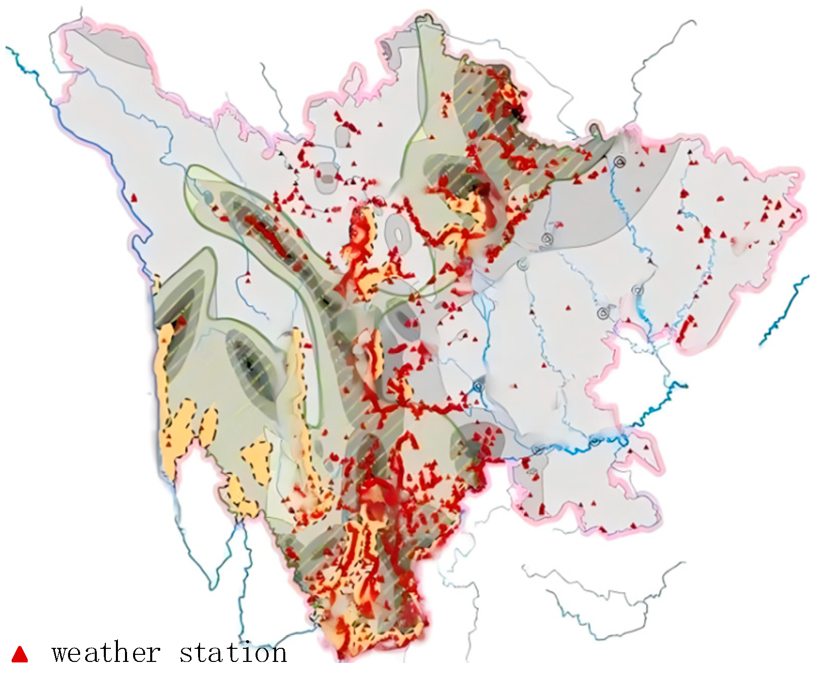
The research data on the rainfall patterns in the study area are all from the China Meteorological Station, with a total of 27 meteorological stations in the study area. The daily rainfall data for the whole year have passed a strict quality inspection, and six stations with missed measurements and observation years of less than 51 years have been excluded. Finally, 21 representative stations were selected to obtain the rainfall data of the undertaking area from these stations. Debris flow is a secondary disaster caused by rainfall, so rainfall data collection affects the final model construction effect. The terrain of the study area is shown in Figure 1.

Figure 1.
Topographic map of the study area.
(2) Geological data collection
In the study area, several measuring points are arranged to collect geological information and geotechnical data, and at the same time, more rigorous geological survey data are obtained from relevant local departments as the basis of model construction.
2.2.2. Multi-Index Rainfall Data Processing Based on Spatial Interpolation
In the acquisition of geological and geotechnical data, spatial interpolation methods play an important role. Usually, various methods such as ground investigation, drilling, geophysical exploration, and geochemical exploration are used to obtain data on ground investigation points, drilling hole locations, geophysical exploration points, geochemical exploration points, and groundwater observation wells. These data acquisition points at different locations together constitute the geological and geotechnical dataset of the study area. Through spatial interpolation methods, these discrete data points can be summarized into a continuous data surface in order to gain a more comprehensive understanding of the geological conditions and geotechnical properties of the study area.
Spatial interpolation is a process of estimating the values of surrounding multi-index points with known point values. It follows Tobler’s geographical law and is also related to the first law of geography. There are various standards of spatial interpolation classification and many types of spatial interpolation methods. Kriging is a widely used spatial interpolation, which is developed in geostatistics. The Kriging spatial interpolation method belongs to the spatial interpolation of random geostatistical analysis. Kriging interpolation is also a process in which the surface generated by accurate interpolation passes through all known observation points, which generally has a good interpolation effect.
The rainfall data obtained from the weather stations in the study area are large in quantity, with the properties of multi-index and strong discreteness, so it is necessary to use the spatial interpolation method to summarize these multi-index discrete rainfall data into data surfaces. The collaborative Kriging spatial interpolation method is a discrete data processing method based on the geostatistics principle, which evolved from the Kriging interpolation method. The Kriging method is based on the spatial distribution structure, using the variogram theory and the spatial variable properties of the original data, to make the optimal unbiased estimation of multi-index regionalization variables [14], and on this basis, to obtain the data surface of the rainfall in the research area. Formula (1) is the basic expression:
In the formula, set is a second-order random function, and the value of is an unknown constant. is the estimated value of the unknown point , is the measured value of the multi-index weather station , and is the weight coefficient of the station to the unknown point.
Kriging interpolates according to the actual spatial variability of the rainfall in the study area, which requires a special geostatistical tool: the semi-variance function, that is, the variation function, which determines the spatial structure characteristics of variables and then affects the weight coefficient . The formula of the variation function is Formula (2):
In the formula, is the value of the variation function, is a space separation distance vector, is the number of sample point pairs separated by , and express the difference in the attribute values between the point and point. When actually processing rainfall data, the exponential model in the Kriging semi-variance fitting model is selected for a detailed calculation:
In the process of estimating the estimation point, it is assumed that the basic conditions of statistical analysis are the following: second-order stationarity and this hypothesis are satisfied, and this method still needs some conditions [15].
(1) Unbiased estimation conditions:
Suppose is the unbiased estimator of , then according to the calculation formula of the unbiased estimator, we can know that:
Because , and at the same time, there are:
So is the unbiased estimation of conditions.
(2) Calculation of weight coefficient
First, we need to derive the ordinary Kriging equations from the formula for estimating the variance:
Among them, is the covariance function of points and , let , , , the estimation variance is minimized through the Lagrange constructor, and the ordinary Kriging equations are obtained through sorting out:
(3) Kriging’s estimation variance is the smallest
At the same time, the minimum form of the estimated variance is also obtained, which is shown as follows:
In the Kriging interpolation process, there is another important parameter—the search radius, which determines the number of interpolation sample points. The radius is controlled mainly by setting the maximum number of searches and the minimum number of samples [16]. In this paper, the maximum number of searches is set to 15, and the minimum number of samples is set to 2.
Based on the Kriging interpolation, the number of regionalized variables is developed from one to many, forming multiple indicators, and the collaborative Kriging method is formed through evolution. The regionalized variable of rainfall information in the study area is introduced into the collaborative Kriging as the second type of information. Equation (10) is the formula of the collaborative Kriging method:
Here, is the interpolation estimation value of the point ; is the observations at stations ; is the elevation value of the point ; is the number of meteorological stations; , are the weights of collaborative Kriging; is the average value of elevation; and is the average value of the meteorological attribute values. The weight of the collaborative Kriging can be calculated through the equation set:
In the formula, , is a Lagrange operator, and is the variation function value at and after the fusion of type I information and type II information. Equation (12) is the expression:
Based on the above derivation process, the third type and the fourth type of information can be added. Based on the ordinary Kriging method, this paper selects three environmental factors related to the rainfall in the study area as the second type of impact factors, the third type of impact factors, and the fourth type of impact factors, and conducts optimization research on the spatial interpolation of rainfall after integrating multiple indicators.
2.2.3. Establishment of Debris Flow Early Warning Model
There is a close relationship between precipitation and debris flow, and heavy rainfall is one of the important triggering factors for the occurrence of debris flow. Precipitation induces the formation of debris flow and affects its activity level. At the same time, precipitation intensity is closely related to the development of debris flow, and vegetation conditions and precipitation jointly affect the probability of debris flow occurrence. Therefore, monitoring and analysis of precipitation are crucial in the early warning and prevention of debris flows. The model calculation is based on the support vector machine. Suppose that the multi-index rainfall data interpolated by space are the training sample in the support vector machine: with represents a sample mapped to a high-dimensional space to representing the corresponding nonlinear mapping, and the function expression constructed is:
Among them, is called the adjustable weight vector, is the offset value, and , are the dimension vector, and to find the optimal classification hyperplane, that is, to find the optimal and due to the existence of the fitting error [17], introduce and as a relaxation variable, and use the -SVR model to establish the following model optimization function with constraints:
Use , as its purpose is to improve the generalization ability of the function, make the function more flat, and increasing the reduces the changes caused by some discrete points in the model, where is called a penalty parameter, which is used to adjust the fitting error beyond the limit degree of punishment , and the larger the discrete point is, the greater the influence of the discrete point on the objective function. Equation (19) is a convex quadratic optimization problem solved by the Lagrange multiplier method, and the Lagrange function is established. , , , and are Lagrange multipliers.
The partial derivative poses zero for and , respectively, and the reverse (14), the corresponding KKT condition can be found, and the quadratic programming optimization algorithm can be used as the training algorithm to calculate the parameters in turn and , and the corresponding optimal multiplier . At the same time, the prediction function is constructed:
The expression of the nonlinear mapping is difficult to determine, so the kernel function Kernel is introduced to equivalent the sum of the inner product squares of the original features to the sum of the inner product squares of the mapped features [18], thus indirectly solving the nonlinear mapping of the kernel functions satisfying the functional Mercer theorem, which can all be regarded as effective kernel functions, among which the radial basis function kernel function has a wide convergence domain, which is the most commonly used kernel function in solving practical problems.
(1) Computation of Quadratic Programming Problem Based on Serial Minimization
Sequential minimal optimization (SMO) is the most effective algorithm for solving quadratic programming problems. As a decomposition algorithm, the SMO algorithm has only two data samples in its algorithm space, and only two Lagrange multipliers need to be optimized for each corresponding operation. Because each Lagrange multiplier is subject to linear constraints, the problem we need to solve is how to realize the optimization of the connected variables and which Lagrange multipliers to choose for optimization [19]. The SMO algorithm is as follows:
① Use the SMO algorithm to construct the corresponding quadratic optimization problem;
② Give all Lagrange multipliers initial values;
③ Judge whether all the Lagrange multipliers meet the KKT conditions, and if they all meet the KKT conditions, then the obtained Lagrange multipliers and b values are the solutions of the quadratic optimization problem, and the algorithm ends, otherwise, the algorithm goes to step ④; Select and judge whether the first Lagrange multiplier meets the KKT condition, and if so, re-select or otherwise select the first multiplier;
④ Select the second Lagrange multiplier, and then solve the optimization problem composed of the two multipliers to obtain the final result of the multiplier;
⑤ Update the Lagrange multiplier and B value, and go to step ③.
Where the KKT condition can be equivalently expressed as Formula (16):
(2) Parameter optimization based on the sea squirt algorithm.
The mudflow warning based on SVM is an optimization problem to determine the optimal penalty parameter and RBF parameter . In this paper, the optimal penalty parameters are determined by the sea squirt algorithm and RBF parameters . The early warning model of debris flow based on the support vector machine (SVM) optimized by the sea squirt algorithm is constructed.
The sea squirt is a small colloid chordate animal in the open sea. Its body is transparent like a barrel, and it moves by absorbing water and spitting water. When it moves in groups, it will form a chain structure. The researchers mathematized this behavior and formed a new swarm intelligence optimization algorithm [20]: the sea squirt algorithm. All the individuals in the sea squirts are distributed among the dimension space, using position matrix to express:
In the formula, is the population number of Styela clava, the first half is the leader and the second half is the follower, and is the position of an individual . The position of the first Styela clava individual (i.e., leader) is updated to:
In the formula, is for food in the position of the dimension; is the upper bound of the dimension search space; is the lower bound of the dimension search space; and are a random number between [0, 1], determines that moving step when the lead iteratively updates, and determines its moving direction; and is to balance the parameters of global search and local development, and the constraint formula is:
In the formula, is the current iteration number and is the maximum number of iterations.
The next iterative updating position of the individual position of the follower of Styela clava is determined by its own previous position and the individual position of the previous Styela clava:
In each iteration, it is assumed that the food position is the individual position of the Styela clava with the best fitness. After many iterations, the whole chain of Styela clava moves to the food position. The sea squirt algorithm is introduced into the support vector machine, and finally the optimal solution of the support vector machine is obtained.
(3) Construction steps of the debris flow early warning model
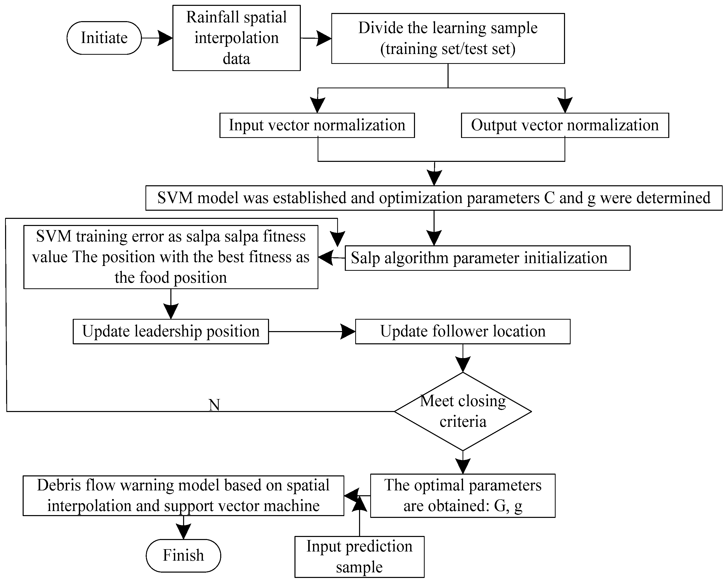
The construction steps of the multi-index fusion debris flow early warning model based on spatial interpolation and the support vector machine are as follows:
① Process the rainfall data of a plurality of meteorological stations with discrete characteristics into a multi-index fused data surface by using a collaborative Kriging space interpolation method;
② Use the sea squirt algorithm to find the optimal parameters of SVM, and construct the optimized support vector machine model of stone flow early warning;
③ The established SVM model is applied to the test samples to realize the early warning of debris flow and output the early warning results of the debris flow.
The steps of the debris flow early warning model are shown in Figure 2.

Figure 2.
Steps of debris flow warning model.
3. Result Analysis
The basic geological conditions and rainfall data are obtained from the study area, and after processing by the method of this paper, a multi-indicator fusion of the debris flow warning model is obtained. Because the debris flow disaster site cannot be actually created in the process of experimental analysis, it is necessary to use the model test software to verify the effect of this model in the early warning of debris flow.
3.1. Rainfall Data Spatial Interpolation Processing Effect
Spatial interpolation simulation is the fitting of a semi-variance function model. The semi-variance function is called the semi-variance function, which is crucial in geostatistics research. Its function fitting also affects the accuracy of the interpolation results and includes three important parameters: lump gold value—variation caused by random factors; base value—variation within the system; range—the range that reflects the autocorrelation of variables; and the spatial correlation degree of the system variables is expressed by the ratio of the lump gold value to the abutment value. Based on the rainfall data from June to September, Table 1 shows the spatial interpolation semi-variance fitting parameter results.

Table 1.
Semi-variance fitting parameters of spatial interpolation.
Based on several important parameters in Table 1, the ordinary Kriging spatial interpolation method and the optimized collaborative Kriging method are used to interpolate the rainfall data in the study area, respectively, and 20 is set as the maximum number of searches, 2 is the number of few samples, and the exponential function selects the semivariogram function. Comparing the two methods, the average absolute error (MA), root mean square error (RMS), and standard root mean square error (RMSS) are obtained by cross-checking the meteorological stations participating in interpolation. The test results are shown in Table 2.
Table 2.
Results of cross-examination.
As can be seen from Table 2, two errors, MA and RMS, characterize the relationship between the actual value and the result value obtained by interpolation, and the RMSS error is used to characterize the effectiveness of the interpolation method. In the comparison of the three errors, on the whole average, the accuracy of the collaborative Kriging method is slightly better than that of the ordinary Kriging method, but the degree of superiority is not very prominent, and the difference between the two interpolation methods in RMS and RMSS is smaller than that of MA. From the time point of view, there is a big difference in MA between June and September, followed by July, and the difference between the two MAs in August is very small.
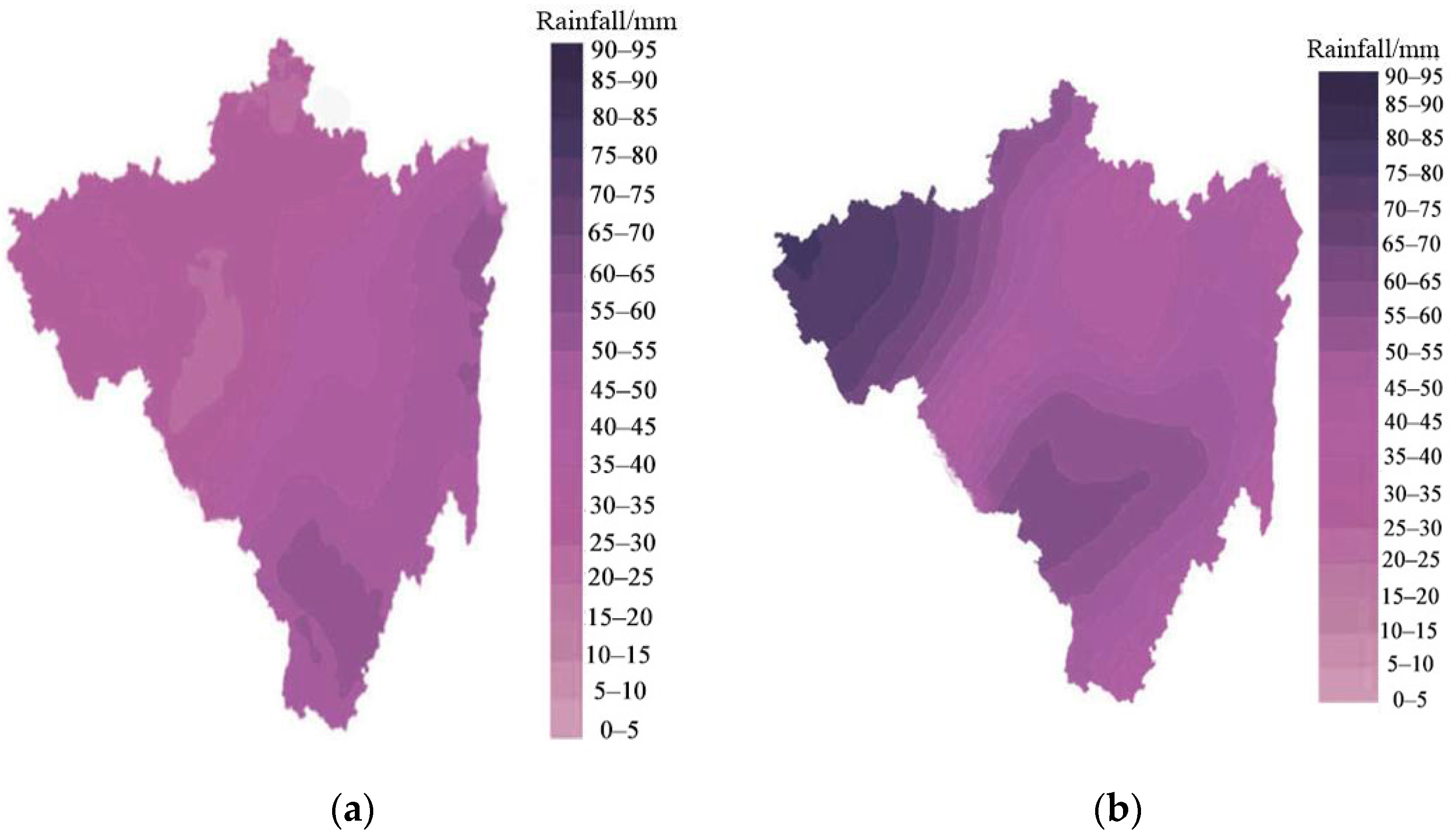
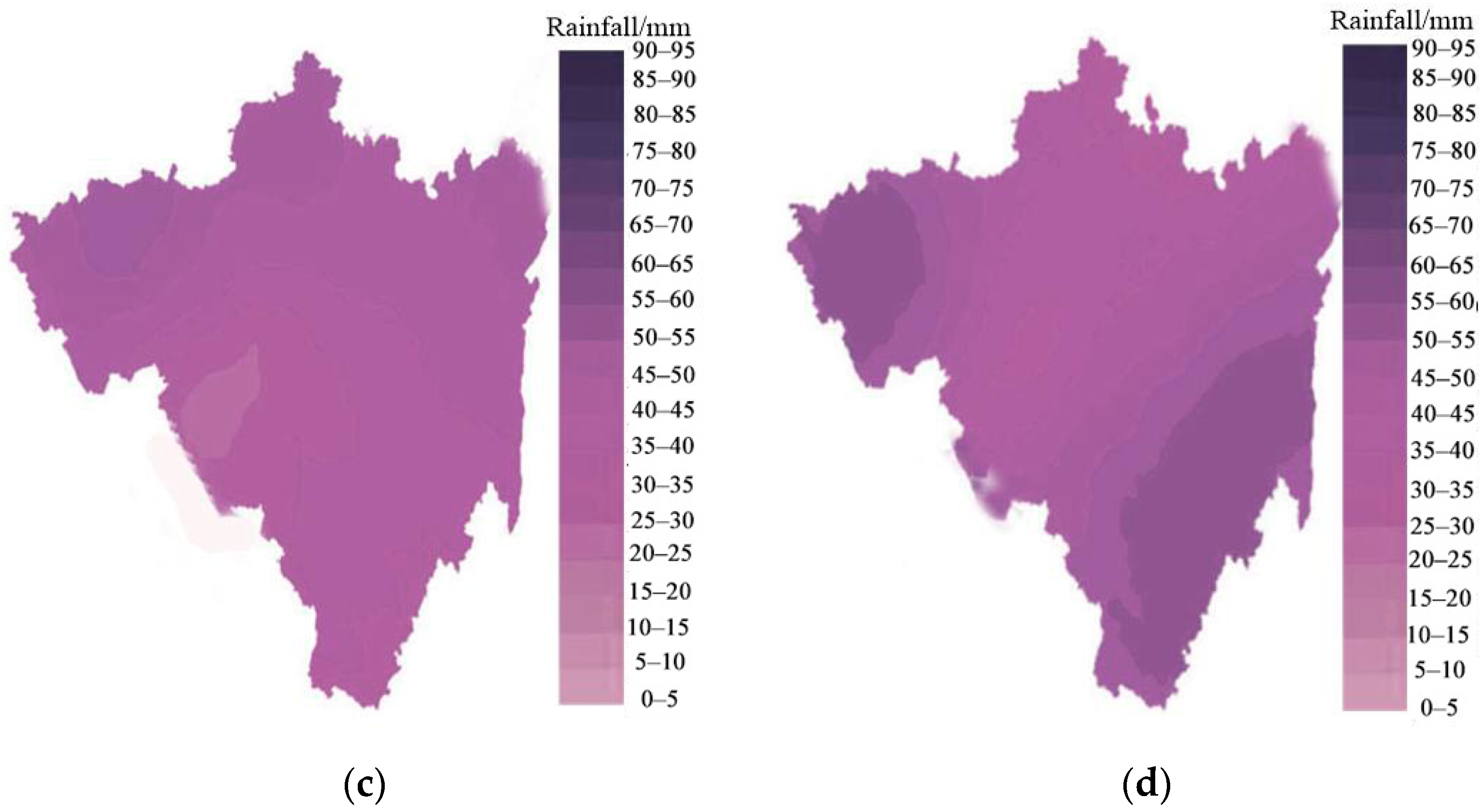
The spatial distribution map of the interpolation results of the average rainfall in the study area from June to September generated by this method is shown in Figure 3.
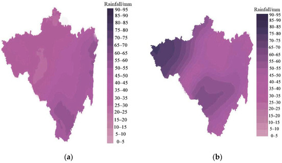

Figure 3.
Spatial interpolation results of precipitation in the study area. (a) June spatial interpolation; (b) July spatial interpolation; (c) August spatial interpolation; (d) September spatial interpolation.
From Figure 3, we can clearly see the spatial distribution of rainfall in the study area, and we can obtain the rainfall distribution accurately and the rainfall situation. And from Figure 3b, we can intuitively see that the rainfall in July is obviously higher than that in June, August, and September, and the spatial interpolation result is consistent with the actual data in the study area, which shows that the spatial interpolation result is effective and accurate.
3.2. Debris Flow Early Warning Model Analysis of Early Warning Results
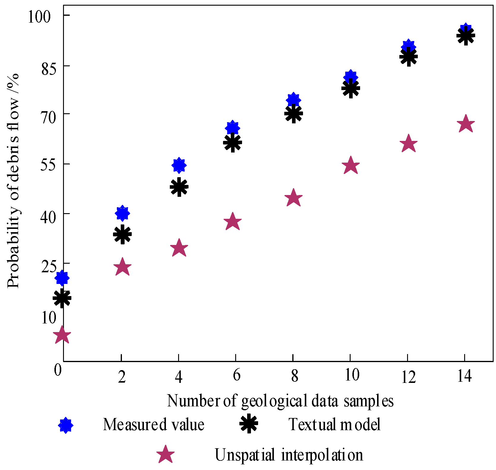
Using this model, the early warning performance of debris flow in the study area is tested, considering the number of rainfall and geological data samples, and the test results are shown in Figure 4.
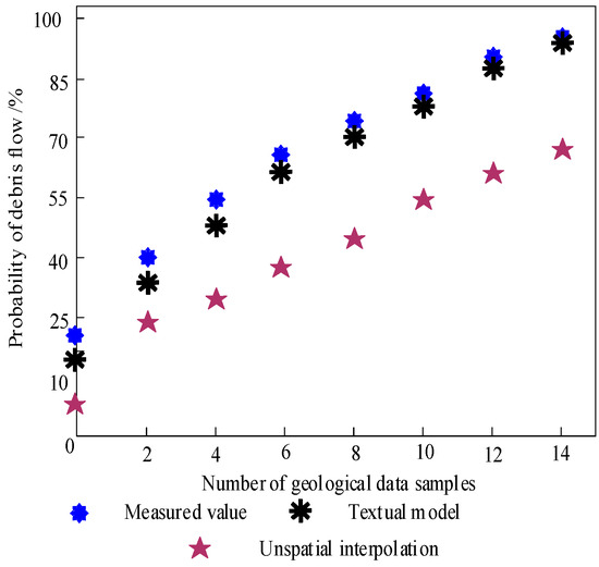
Figure 4.
Test of debris flow warning model.
As a whole, Figure 4 shows that the more samples of rainfall data and geological data obtained from the study area, the closer the value of this early warning model is to the actual data of debris flow, but the early warning trend of the model without spatial interpolation is not obvious, which is also related to the number of samples, which once again shows that this model is more suitable for debris flow data processing with small sample characteristics. At the same time, the early warning result of this model is close to the actual value, which shows that it is possible to apply this model to the probability prediction of debris flow, and this model can accurately obtain the change in the debris flow in the study area and obtain more effective early warning results.
In order to further verify the early warning effect of this model, several debris flow gullies in the study area are numbered 1–10, and the actual times of the debris flow in each debris flow gully in this area in recent ten years are counted. At the same time, this model and the early warning model using only a support vector machine without spatial interpolation are used to provide an early warning of the debris flow in the study area, the number of debris flows warned is counted, and whether there is a difference between the warning times and the actual times of debris flow is compared. The test results are shown in Table 3.
Table 3.
Comparison of warning times.
From the test results in Table 3, it can be seen that the early warning results of this model are close to the actual results of the debris flows, and the number of actual occurrences of debris flows in each debris flow is basically consistent with the early warning results, which shows that the early warning results of this model have high accuracy, are accurate enough to warn the occurrence of debris flows in the study area, have been referenced, and can be popularized and used in many areas in the future.
4. Conclusions
In this paper, a multi-indicator fusion mudslide early warning model based on spatial interpolation and the support vector machine is studied. The rainfall data of the study area are processed by using synergistic Kriging spatial interpolation, the geological data of the study area are processed by means of principal component analysis, the mudslide early warning model is constructed after the fusion of multi-indicators by the support vector machine, and the possibility of outbreaks of mudslides is forewarned by using the model. Simulation experiments were carried out with the historical data of the study area, and the results of the early warning model used in the study and the model without spatial interpolation were compared, respectively. Mudslide prediction is a complex system with serious nonlinearity under the combined effect of rainfall conditions, geological conditions, and other conditions, so the application of principal component analysis and spatial interpolation in the multi-indicator fusion of the support vector machine model, compared with the previous use of neural networks, machine learning, and fuzzy analysis theory, can not only effectively deal with the correlation and sensitivity of factors, but also reflect the correlation and sensitivity of the factors in a more objective way. It can not only effectively deal with the correlation and sensitivity between the factors, but also more objectively reflect the relationship between the disaster-causing factors and the mudslide disaster, and minimise the influence of human factors on the prediction effect of the model.
However, the model still has some limitations, such as region-specific adaptation, the generalisation ability of the model, and how to handle more influencing factors. Future research could further optimise the model, for example, by integrating more types of data, improving spatial interpolation methods, or using new techniques such as deep learning. Nevertheless, the model still provides a powerful tool for the early warning of mudslide disasters, and offers new ideas and methods for research and practice in related fields.
Author Contributions
Software, S.W.; Formal analysis, S.W.; Investigation, S.W.; Writing—original draft, R.J.; Writing—review & editing, S.W. and J.L. All authors have read and agreed to the published version of the manuscript.
Funding
This research received no external funding.
Data Availability Statement
Data are contained within the article.
Conflicts of Interest
The authors declare no conflict of interest.
References
- Luo, H.; Zhang, L.; He, J.; Yin, K. Reliability-based formulation of building vulnerability to debris flow impacts. Can. Geotech. J. 2022, 59, 40–54. [Google Scholar] [CrossRef]
- Kattel, P.; Khattri, K.B.; Pudasaini, S.P. A multiphase virtual mass model for debris flow. Int. J. Non-Linear Mech. 2021, 129, 103638. [Google Scholar] [CrossRef]
- Takayama, S.; Satofuka, Y.; Imaizumi, F. Effects of water infiltration into an unsaturated streambed on debris flow development. Geomorphology 2022, 409, 108269.1–108269.12. [Google Scholar] [CrossRef]
- Wang, D.; Wang, X.; Chen, X.; Lian, B.; Wang, J. Analysis of factors influencing the large wood transport and block-outburst in debris flow based on physical model experiment. Geomorphology 2022, 398, 108054. [Google Scholar] [CrossRef]
- Piciullo, L.; Tiranti, D.; Pecoraro, G.; Cepeda, J.M.; Calvello, M. Standards for the 840 performance assessment of territorial landslide early warning systems. Landslides 2018, 17, 2533–2546. [Google Scholar] [CrossRef]
- Sättele, M.; Bründl, M.; Straub, D. Reliability and effectiveness of early warning systems for natural hazards: Concept and application to debris flow warning. Reliab. Eng. Syst. Saf. 2015, 142, 192–202. [Google Scholar] [CrossRef]
- Tiranti, D.; Cremonini, R.; Marco, F.; Gaeta, A.R.; Barbero, S. The DEFENSE (debris Flows triggEred by storms—Nowcasting system): An early warning system for torrential processes by radar storm tracking using a Geographic Information System (GIS). Comput. Geosci. 2014, 70, 96–109. [Google Scholar] [CrossRef]
- Vaughn, T.; Crookston, B.M.; Pfister, M. Floating woody debris: Blocking sensitivity of labyrinth weirs in channel and reservoir applications. J. Hydraul. Eng. 2021, 147, 06021016. [Google Scholar] [CrossRef]
- Baggio, T.; Mergili, M.; D’Agostino, V. Advances in the simulation of debris flow erosion: The case study of the Rio Gere (Italy) event of the 4th August 2017. Geomorphology 2021, 381, 107664. [Google Scholar] [CrossRef]
- Bernard, M.; Gregoretti, C. The use of rain gauge measurements and radar data for the model-based prediction of runoff-generated debris-flow occurrence in early warning systems. Water Resour. Res. 2021, 57, e2020WR027893. [Google Scholar] [CrossRef]
- Palucis, M.C.; Ulizio, T.P.; Lamb, M.P. Debris flow initiation from ravel-filled channel bed failure following wildfire in a bedrock landscape with limited sediment supply. GSA Bull. 2021, 133, 2079–2096. [Google Scholar] [CrossRef]
- Tsunetaka, H.; Hotta, N.; Imaizumi, F.; Hayakawa, Y.S.; Masui, T. Variation in rainfall patterns triggering debris flow in the initiation zone of the Ichino-sawa torrent, Ohya landslide, Japan. Geomorphology 2021, 375, 107529. [Google Scholar] [CrossRef]
- Kovářík, K.; Mužík, J.; Masarovičová, S.; Bulko, R.; Gago, F. The local meshless numerical model for granular debris flow. Eng. Anal. Bound. Elem. 2021, 130, 20–28. [Google Scholar] [CrossRef]
- Zandi, O.; Nasseri, M.; Zahraie, B. A locally weighted linear ridge regression framework for spatial interpolation of monthly precipitation over an orographically complex area. Int. J. Clim. 2023, 43, 2601–2622. [Google Scholar] [CrossRef]
- Das, S. Wahiduzzaman Identifying meaningful covariates that can improve the interpolation of monsoon rainfall in a low-lying tropical region. Int. J. Clim. 2021, 42, 1500–1515. [Google Scholar] [CrossRef]
- Saha, A.; Gupta, B.S.; Patidar, S.; Martínez-Villegas, N. Spatial distribution based on optimal interpolation techniques and assessment of contamination risk for toxic metals in the surface soil. J. South Am. Earth Sci. 2022, 115, 103763. [Google Scholar] [CrossRef]
- Li, X.; Li, J.; Xia, Z.J.; Georgakarakos, N. Machine-learning prediction for mean motion resonance behaviour—The planar case. Mon. Not. R. Astron. Soc. 2022, 511, 2218–2228. [Google Scholar] [CrossRef]
- Jiang, W.; Xie, Y.; Li, W.; Wu, J.; Long, G. Prediction of the splitting tensile strength of the bonding interface by combining the support vector machine with the particle swarm optimization algorithm. Eng. Struct. 2021, 230, 111696. [Google Scholar] [CrossRef]
- Guo, B.; Zhang, X.; Cui, J. Segmentation of Inhomogeneous Images Using Improved Symmetric Active Contour Model. Comput. Simul. 2023, 40, 227–233. [Google Scholar]
- Guo, Z.; Tian, Y.; Feng, Y.; Zhang, H.; Liu, J.; Wang, Z. Salp swarm algorithm based on golden section and adaptive and its application in target tracking. IET Image Process. 2022, 16, 2321–2337. [Google Scholar] [CrossRef]
Disclaimer/Publisher’s Note: The statements, opinions and data contained in all publications are solely those of the individual author(s) and contributor(s) and not of MDPI and/or the editor(s). MDPI and/or the editor(s) disclaim responsibility for any injury to people or property resulting from any ideas, methods, instructions or products referred to in the content. |
© 2024 by the authors. Licensee MDPI, Basel, Switzerland. This article is an open access article distributed under the terms and conditions of the Creative Commons Attribution (CC BY) license (https://creativecommons.org/licenses/by/4.0/).