Abstract
Nonpoint source pollution (NPS) has become the most important reason for the deterioration of water quality, while relevant studies are often limited to African river and lake basins with insufficient data. Taking the Simiyu catchment of the Lake Victoria basin as the study area, we set up a NPS model based on the soil and water assessment tool (SWAT). Furthermore, the rationality of this model is verified with the field-measured data. The results manifest that: (1) the temporal variation of NPS load is consistent with the variation pattern of rainfall, the average monthly output of total nitrogen (TN) and total phosphorus (TP) in the rainy season was 1360.6 t and 336.2 t, respectively, while in the dry season was much lower, only 13.5 t and 3.0 t, respectively; (2) in view of spatial distribution among 32 sub-basins, TN load ranged from 2.051 to 24.288 kg/ha with an average load of 12.940 kg/ha, and TP load ranged from 0.263 to 8.103 kg/ha with an average load of 3.321 kg/ha during the 16-month study period; (3) Among the land use types, the cropland contributed the highest proportion of TN and TP pollution with 50.28% and 76.29%, respectively, while the effect of forest on NPS was minimal with 0.05% and 0.02% for TN and TP, respectively. (4) Moreover, the event mean concentration () values of different land use types have been derived based on the SWAT model, which are key parameters for the application of the long-term hydrological impact assessment (L-THIA) model. Therefore, this study facilitates applying the L-THIA model to other similar data-deficient catchments in view of its relatively lower data requirement.
1. Introduction
Nowadays, point source pollution has been effectively controlled, while nonpoint source pollution (NPS) has become one of the most important reasons resulting in the deterioration of the surface water environment. However, NPS assessment is usually limited for insufficient monitoring data in some areas.
As the largest tropical lake in the world, Lake Victoria has a basin area of 193,000 km2 and a water area of about 68,800 km2 [1]. The lake water is shared by Kenya, Tanzania, and Uganda, and the lake basin covers parts of Burundi, Kenya, Rwanda, Tanzania, and Uganda [2]. The Lake Victoria basin is one of the most densely populated areas in Africa. It is estimated that between 2000 and 2010, the population of this basin increased from 54.5 to 73.6 million people who directly or indirectly relied on Lake Victoria for survival and development [3,4]. The lake is also home to a variety of flora and fauna [5]. Rapid population growth in the past few decades, coupled with the continuous expansion of agricultural and urban land, has put great pressure on the water quality of Lake Victoria [6,7]. Due to the deficiencies in the environmental management systems, untreated emissions from domestic garbage, sewage, agricultural pesticides, and fertilizers have been prevalent in the highly populated areas around the lake, leading to serious eutrophication of Lake Victoria [8,9]. As a result, the ecosystem within the lake and the safety of drinking water in the lake zone have been seriously affected [10,11,12,13]. According to a five-year (1997–2002) management experience of the Lake Victoria Environmental Management Project (LVEMP), launched unitedly by Kenya, Tanzania, and Uganda in 1994, NPS has become the major contributor to the deterioration of water quality in Lake Victoria [14]. With the effective control of point source pollution, more scholars now focus on NPS in the Lake Victoria basin [15,16].
NPS in Lake Victoria has become an important factor limiting the sustainable water quality management of this basin. Therefore, relevant research such as the quantification of pollution load and the analysis of pollution output characteristics is beneficial to the ecological and environmental protection of Lake Victoria. At present, the model method is often used to study NPS [17,18,19]. Among numerous models, the soil and water assessment tool (SWAT) has a wide range of successful applications in the field of NPS research [20,21]. The SWAT model is composed of a hydrological cycle module, a soil land erosion module, and a pollutant load module, which can simulate runoff, sediment, nutrients, and other transport processes in the basin [22,23,24]. The data input to the SWAT model mainly includes the digital elevation model (DEM), land use, soil and meteorological data, and output runoff and nutrient data of the river cross-section and basin. Because it can fully consider the hydrological cycle and nutrient migration process and can make full use of spatial data by combining with other models or methods, SWAT could be applied to a wider range of research fields [25,26].
The SWAT model is mainly based on the water balance equation, which is the driving force for all processes in the basin. High-quality hydrological and water quality monitoring data are critical in the calibration and validation of SWAT parameters. However, there are relatively few hydrological stations in Africa [27,28]; and accurately measured hydrological and water quality data only exist in a few cities in African countries such as Niger and Togo [16]. Therefore, the lack of data has hindered the application of SWAT in the Lake Victoria basin, though a few related studies existed. For example, Kimwaga et al. [29] simulated the NPS in the Simiyu catchment in Tanzania using the SWAT model. The results from the study indicated an underestimation of the sediment production because only seven sediment monitoring data were used to calibrate the SWAT parameters, which were insufficient. Another study from Cheruiyot and Muhandiki [30] failed to obtain ideal simulation results of the NPS in the Sondu watershed in Kenya due to less and discontinuous water quality data. As a result, obtaining reliable simulation results with insufficient data has become a central challenge to researchers trying to simulate current or future NPS in the Lake Victoria Basin.
Unlike SWAT, the long-term hydrological impact assessment (L-THIA) model, which was jointly developed by the U.S. Environmental Protection Agency (EPA) and Purdue University, has relatively lower requirements for data and is more applicable in data-poor areas and situations [31,32]. The core of the L-THIA model is the classic SCS-CN model, so the long-term rainfall, soil, and land use data are used to simulate runoff volume [33,34]. The output data include the runoff and total NPS load of different land use types. The event mean concentration () is the critical parameter of the L-THIA model to simulate NPS loads. However, numerous studies have shown that the default values should be localized. For example, when studying the AXL watershed located in DeKalb County, Northeastern Indiana state, Liu et al. [35] expressed that total nitrogen (TN) and total phosphorus (TP) loads simulated using the default values were relatively small. Nejadhashemi et al. [36] indicated that because the default values were too small, the NPS of the Pomona Lake watershed in North-east Kansas state simulated by the L-THIA model was also too small, and if accurate values could be obtained, nitrogen and phosphorus pollution in this watershed would be well simulated. So far, no scholars have applied the L-THIA model to the Lake Victoria basin to study NPS, and there are no relevant values to be defined in this region. If we select a catchment with relatively complete data to build the SWAT model and use the high temporal resolution flow and non-point source data obtained from the model simulation, the required parameters can be derived for L-THIA model construction. Thus, the innovative integrated use of these two models is expected to achieve NPS simulation in data-deficient areas.
The Simiyu catchment is located in the southeast of Lake Victoria. The increasing population and the development of economic activities such as agriculture and livestock have exacerbated nutrient pollution in this catchment, resulting in severe deterioration of water quality [37]. As an important channel into Lake Victoria, the Simiyu River accounts for 4.6% of the total annual lake flux and collects and delivers a large share of NPS into Lake Victoria [38,39]. Besides, the Simiyu catchment is a typical agricultural catchment in the area around Lake Victoria, and the agricultural activities in this catchment strongly affect the lake characteristics in the southeast [40]. Therefore, controlling the NPS of the Simiyu catchment is key to improving the water quality of both the Simiyu River and Lake Victoria. Currently, there are no monitoring activities in the Simiyu catchment or in the entire Lake Victoria Basin. Thus, the application of the L-THIA model in this area would be difficult.
In this article, we analyze the temporal and spatial distribution characteristics of the nonpoint source TN and TP pollution in the Simiyu River catchment; the values of TN and TP pollution for different land use types are also derived based on the SWAT model. The results of this study are expected to provide a relevant reference for the management of NPS, both currently and in the future, not only in the Simiyu catchment but also in other similar catchments with poor or no data.
2. Materials and Methods
2.1. Conceptual Framework
The schematic flow chart as shown in Figure 1 provides the conceptual framework of this study. First, the SWAT model suitable for Simiyu catchment was constructed based on DEM, land use and land cover (LULC), soil, meteorological and other basic data. Then, the SWAT model was used to simulate the TN and TP pollution in the Simiyu catchment. Further, the values of TN and TP pollution for different land use types in the Simiyu catchment were derived by combining SWAT and L-THIA models.
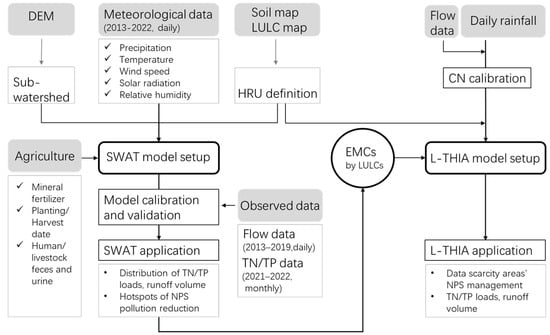
Figure 1.
Flow chart of this study (the abbreviations of LULC standing for land use and land cover; HRU for hydrologic response unit; CN for runoff curve number; NPS for nonpoint source pollution).
2.2. Study Area
The Simiyu catchment is located in the southeast of Lake Victoria between 33°15′ and 35°00′ E and 2°15′ and 3°30′ S, as shown in Figure 2, covering an area of approximately 10,510 km2. The topography of this catchment is low in the west and high in the east, with an elevation range of 1133~2004 m. It is estimated that there are approximately more than 800,000 inhabitants in this catchment area, and its land cover types are dominated by cropland, grassland, and shrubland, with sandy loam, loam, and sandy clay loam as the main soil types. The dense population is usually accompanied by extensive cropland and a large number of livestock and poultry. This catchment is dominated by activities such as subsistence agriculture, livestock and poultry farming, grazing, and these activities put pressure on the land in the Simiyu catchment, resulting in the reduction of forestland as well as soil erosion. The agricultural practices and livestock overgrazing in the Lake Victoria basin have significantly caused environmental degradation over the past few decades [41]. The Simiyu catchment has a savanna climate with an annual average temperature of about 23 °C and distinct wet and dry seasons. The annual average total rainfall is between 700 and 1000 mm, of which 41% occurs in the short rainy season and 39% in the long rainy season [42]. In addition, river flow is high during the rainy season while very low or even zero during the dry season.
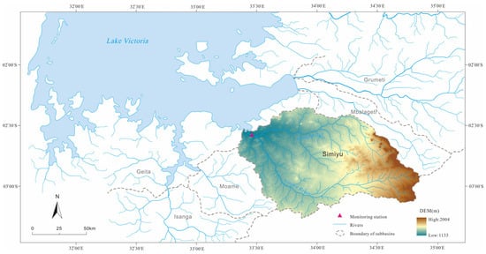
Figure 2.
Location of Simiyu Catchment.
2.3. Data Source
The data used to construct the NPS model for Simiyu catchment is divided into two types, namely spatial data and attribute data. The spatial data include digital elevation model (DEM), land use and land cover data and soil data of the Simiyu catchment, while the attribute data mainly comprise meteorological, hydrological and water quality data, and agriculture management information.
DEM The topographic data used in this study was derived from the Shuttle Radar Topography Mission (SRTM) dataset with a spatial resolution of 90 m, which was processed to obtain the DEM data for Simiyu catchment.
Land use/cover This study used a set of 10 m spatial resolution global surface cover product FROM-GLC10-2017, developed by Gong et al. [43] from Tsinghua University, China. This global land cover map was produced mainly based on Sentinel-2 images with a random forest classifier, and the overall accuracy was 72.76%. The land use/cover reclassification results are shown in Figure 3a, in which cropland area accounts for about 24.33%, grassland area for about 36.97%, shrubland area for the largest proportion, about 38.41%, the area of forest and urban land accounts for a relatively small proportion, 0.14% and 0.11%, respectively, and water body area accounts for only 0.05%.
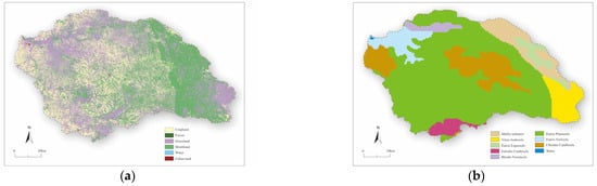
Figure 3.
Distribution of land use (a) and soil types (b) in the Simiyu catchment (land uses: Cropland, Forest, Grassland, Shrubland, Water, Urban land; Soil types: Mollic Solonetz, Vitric Andosols, Eutric Leptosols, Ferralic Cambisols, Rhodic Ferralsols, Eutric Planosols, Eutric Vertisols, Chromic Cambisols, Water bodies).
Soil data Referring to the construction method of the SWAT model soil database discussed by Jiang et al. [44], the soil database for the Simiyu catchment was established based on the publicly available World Soil Database (HWSD). Related software was used for auxiliary calculation, such as SPAW software (6.02.75) to judge the hydrological soil types. The result is shown in Figure 3b.
Meteorological data The meteorological data required for SWAT model construction mainly included the daily precipitation, maximum and minimum temperature, wind speed, relative humidity, and solar radiation, among which the climate hazards group infrared precipitation with station data (CHIRPS) dataset was used for the daily precipitation, and the fifth generation (ERA5) of the European Centre for Medium-Range Weather Forecasts (ECMWF) reanalysis dataset for global climate and weather was used for the other. The meteorological data used to predict the output of NPS from 2023 to 2050 were from the TaiESM1 and FGOALS-g3 models of CMIP6, and the precipitation simulated by TaiESM1 and the temperature simulated by FGOALS-g3 were in good agreement with the measured results in East Africa [45,46].
Hydrological and water quality data Hydrological and water quality data were mainly used for model calibration. The hydrological and water quality observation data used in this article were all sourced from the monitoring station near the outlet of the Simiyu catchment, with the specific location shown in Figure 2. The daily runoff data of the monitoring station from 2013 to 2019 were used. Monthly water quality data (TN and TP concentration) from April 2021 to July 2022 were used in the analysis.
Agriculture information The basic information for Simiyu catchments, such as population, livestock, and poultry production data, was all sourced from the Tanzania National Bureau of Statistics [47]. Crop planting types, planting and harvest dates, fertilizer, and fertilization dates were obtained by the field investigation in 2021.
2.4. Research Methods
2.4.1. SWAT Modeling
The latest version, SWAT 2012, was selected for this simulation. The pre-processed data were input into the SWAT model. Based on DEM and river network data, this model divided the Simiyu catchment into 32 sub-basins by adopting the model recommendation threshold and manually adding the hydrological and water quality monitoring station. The SWAT model further divided the 32 sub-basins into 454 hydrological response units (HRUs) by combining land use, soil types, and slope values.
2.4.2. Calibration and Validation of SWAT Model
The SWAT-CUP software (5.2.1.1) was used for the calibration of the parameters in order to reduce the uncertainty of the SWAT model. In this article, the commonly used SUFI2 algorithm that is integrated into the software was chosen to perform the sensitivity analysis of the parameters as well as the parameters calibration. The validity of the model was evaluated by using the coefficient of determination (), Nash-Sutcliffe efficiency coefficient (), and percent bias () [48]. The calculation formulas are as follows:
where: is the observed flow; is the average value of the observed flow; is the simulated flow; is the average value of the simulated flow.
The results of previous studies [49,50] indicate that hydrologic modeling results are considered reliable when > 0.60, > 0.50 and around ±25%, and water quality modeling results are considered reliable when > 0.6, > 0.50 and around ±40%.
The monthly average flow data from 2013 to 2016 were used for calibration, while the monthly average flow data from 2017 to 2019 were used for validation. Using the water quality data from the monitoring station for the calibration of the pollution module, this article mainly studied TN and TP indicators. Based on the limited monitoring data, June and December of 2018, December 2019, and from April to December 2021 were set as the calibration period, and from January to July in 2022 were set as the validation period.
2.4.3. Derivation of Values for L-THIA Model
The L-THIA model can simulate the contribution of nonpoint source TN and TP for different land use types. The formula used for the L-THIA model is as follows [51]:
where: is the load of nonpoint source pollution (kg); is the average concentration of events for each land use type (mg/L); is the total amount of surface runoff (); and is the unit conversion factor.
The default parameters should be corrected before simulating with the L-THIA model, particularly in areas other than the United States. Generally speaking, the values are obtained based on actual monitoring, which requires a lot of cost. So far, no scholars have monitored the values of the Simiyu catchment. Therefore, in this article, we derived the values suitable for the Simiyu catchment based on Formula (4) and the simulated and by the localized SWAT. Each land use type of every sub-basin delineated by the SWAT was treated as a calculation unit. Then, the mean values of were derived for different land use types. On the other hand, the L-THIA model was set up based on a land use/cover map, soil map, and the adjusted CN of the Simiyu catchment. Then, the obtained were adopted to replace the default ones of L-THIA. The relative errors of the simulation result from the L-THIA model compared with that from the SWAT model were calculated in order to verify the rationality of the derived , as demonstrated in the study by Jiang et al. [52].
3. Results
3.1. Model Calibration and Validation
The results of hydrological calibration and validation of the SWAT model for the Simiyu catchment are listed in Table 1, which meet the accuracy requirements of SWAT model. Figure 4 shows the comparison between the simulated and measured monthly average flow values, which manifests that the simulated curve is basically consistent with the measured curve, indicating that the hydrological simulation results are reasonable and acceptable.

Table 1.
Evaluation of hydrological simulation results by the SWAT model.
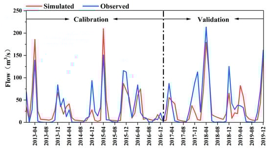
Figure 4.
Comparison of the simulated and measured monthly average flow of the Simiyu River.
The calibration and validation results of TN and TP are summarized in Table 2, which meet the accuracy requirements, indicating that the model has good applicability in the Simiyu catchment. The of TN and TP in the validation period is relatively high because the model significantly underestimates the nitrogen and phosphorus output in January 2022 (Figure 5). In general, the effect of water quality simulation is lower than that of hydrology simulation.
Table 2.
Evaluation of water quality simulation results by the SWAT model.
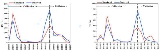
Figure 5.
Comparison of the monthly average simulated and measured values of TN and TP.
In summary, the SWAT model, after calibration and validation, has shown good simulation results for the hydrological and water quality in the Simiyu catchment, so relevant research on nitrogen and phosphorus pollution can be conducted on this basis. Fifteen (15) sensitivity parameters have been determined, as shown in Table 3.
Table 3.
Model parameter calibration values of the SWAT model.
3.2. Analysis of Temporal Variation of NPS
Figure 6 presents temporal distribution characteristics of rainfall (bars) and TN and TP outputs (line plots) analyzed from the simulation results of the Simiyu catchment for the period from April 2021 to July 2022. Figure 6a shows that during the simulation period (16 months), TN output changes from 0.328 to 2978 t, increasing during the rainfall seasons (from December to February and from April to May) while decreasing during the dry season (June to October). Moreover, the average monthly output of TN in the rainy season and the dry season is 1360.6 t and 13.5 t, respectively. The maximum output of the TN value occurred in April 2021, with the highest rainfall. The trend of TN output consistently follows the rainfall trend, indicating that the two are closely dependent. Similarly, TP output follows a pattern consistent with that of TN output (Figure 6b), and the average monthly output of TP in the rainy season and the dry season is 336.2 t and 3.0 t, respectively; however, the TP output (range: 0.009 to 711.1 t) is significantly smaller than the TN output. Rainfall is, thus, a key factor affecting the TN and TP outputs. During the rainy season, the output of nitrogen and phosphorus pollutants from the catchment increases through rainfall-runoff, but they are retained in the system during the dry season when rainfall significantly decreases; thus, the output of nitrogen and phosphorus pollutants decreases accordingly. In addition, although the rainfall in January 2022 is lower than that in February, the output of nitrogen and phosphorus in that month is relatively higher, which may be related to the fertilizer applied in January.
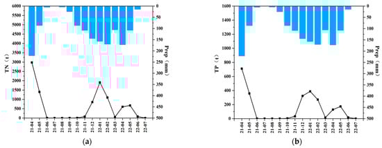
Figure 6.
Monthly variations of rainfall (bars) and output (line plots) of TN (a) and TP (b) at the outlet of Simiyu catchment.
The simulated prediction results of the monthly average rainfall (bars) and outputs of TN and TP (line plots) of the Simiyu catchment during the period from 2023 to 2050 are shown in Figure 7. The average monthly output of TN is still greater than that of TP in the Simiyu catchment, and the two indicators manifest the same change tendency; that is, the output increases in the rainy season while it decreases in the dry season. The sum of TN and TP outputs during rainy season months (4, 5, 12, 1, 2) accounts for 76.63% and 70.56% of those of the whole year, respectively. The simulation results show that the rainy season is a critical period for NPS control, and effective measures should be considered to prevent and reduce NPS during the season. However, during the study period from April 2021 to July 2022, the TN and TP proportion of the rainy season accounted for 95.8–98.2% and 94.9–97.5% of the whole year, respectively (Figure 6). By comparing the results for the two periods, we can find that the proportion of TN/TP outputs in the rainy season might show a nonnegligible reduction in the future. Therefore, the growth of NPS in the traditional dry season should also be taken seriously, and more attention should be paid to the prevention and control of NPS in the dry season as well as in the rainy season in the future.
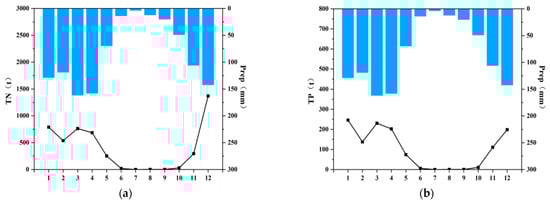
Figure 7.
Monthly variations of TN (a), TP (b) outputs (line plots), and rainfall (bars) predicted for the period from 2023 to 2050 at the outlet of Simiyu catchment.
3.3. Analysis of Spatial Distribution of NPS
When applying the SWAT model, the Simiyu catchment was divided into 32 sub-basins. The load of NPS in each sub-basin is represented by the load per unit area from April 2021 to July 2022, and the calculation results are shown in Figure 8. There are significant differences in nitrogen and phosphorus loads among the sub-basins of the Simiyu catchment. TN load ranges from 2.051 to 24.288 kg/ha with an average load of 12.940 kg/ha, while the TP load ranges from 0.263 to 8.103 kg/ha with an average load of 3.321 kg/ha. Through comparison, it is found that sub-basins 3, 4, 6, 8, and 10 are areas with high TN and TP loads. Compared with other sub-basins, the water yield of sub-basins 3, 4, 6, 8, and 10 is larger, and nitrogen and phosphorus pollutants are prone to enter the river with runoff. Among them, the proportion of cropland area in sub-basins 6 and 8 is larger than that in other sub-basins, and pollutants easily run off into the water body with sediment due to improper cultivation or other reasons. Overall, the distribution characteristics of TN and TP in each sub-basin of Simiyu catchment are relatively quite similar, with pollution in the downstream area of the catchment heavier than that in the upstream area. That might be closely related to the situation that cropland and urban land are mostly distributed in the downstream basin of Simiyu, while forest and shrubland are mostly located in the upstream basin of Simiyu.
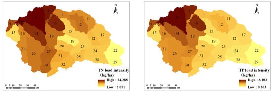
Figure 8.
Spatial distribution of TN and TP loads by the SWAT model in the Simiyu catchment from April 2021 to July 2022 (With the numbers denoting the sub-basins).
The TN and TP loads of each land use type in the Simiyu catchment have been analyzed, and the results are summarized in Table 4. In terms of TN and TP loads, the decline order is cropland > grassland > shrubland > urban land > forest. Although cropland only accounts for 24.33% of the area of the Simiyu catchment, it contributes 50.28% of TN and 76.29% of TP, which is mainly related to the application of fertilizers in the cropland. The nitrogen and phosphorus pollutants are easily flowed away along with runoff and sediment during heavy rainfall due to improper fertilization and soft soil texture. The forest has the least contribution to the TN and TP, mainly because the forest has been less affected by human activities; in addition, the forest plays the role of soil and water conservation, which can accordingly reduce the loading of nitrogen and phosphorus downstream.
Table 4.
The TN and TP contribution of each land use type during the period from April 2021 to July 2022.
3.4. Derivation Results of Values
Based on the simulated TN, TP, and runoff volume with the SWAT model, the values of different land use types have been derived in the 32 sub-basins of the Simiyu catchment, with the results summarized in Table 5. Among the land use types, cropland has the highest TN concentration of 10.74 mg/L, which is related to the applied nitrogen fertilizers. In contrast, the TP concentration of cropland is lower than that of urban land, which is strongly related to human domestic sewage as well as livestock and poultry keeping. In addition, phosphorus is usually found to be adsorbed onto fine sediment particles. Urban land lacks vegetation that plays the role of soil and water conservation. Thus, phosphorus will run off along with sediment during heavy rainfall. Among all land use types, the value of forest is the lowest, which again verifies the interception effect of forest on nitrogen and phosphorus pollutants. Therefore, the importance of forest protection is even more prominent.
Table 5.
Derivation results of values based on the SWAT model in the Simiyu catchment.
4. Discussion
4.1. Rationality of Simulation Results
The hydrological calibration and validation results of the SWAT model meet the standards, and the model captures both high and low-flow seasons well (Figure 4). The simulated monthly flow ranges from 1.08 to 226.4 m3/s for the period from 2013 to 2019 at the outlet of the Simiyu catchment, which is consistent with the monthly flow range from 1981 to 1991 [53], as well as the flow ranges observed during the period from 2013 to 2019. Moreover, the nitrogen and phosphorus simulation evaluation results also show that the model meets the requirements for water quality simulation application (Table 2). However, it should be pointed out that the SWAT model underestimates the output of TN and TP in rainy seasons, probably due to the unusually heavy rainfall events in these months, as has been indicated in other previous studies [54]. In general, the hydrological and water quality simulation results by the SWAT model are reasonable and better than previous reports on this region. For example, Kimwaga et al. [55] reported the value of for hydrologic simulation results to be 0.345 and 0.301, respectively, during calibration periods and validation periods in the same Simiyu catchment. Also, Cheruiyot and Muhandiki [30] reported the value in the Sondu catchment of Kenya to be 0.46 and −4.45, respectively. The values of both cases are significantly lower than reported in the current study (Table 1). The value of obtained by Cheruiyot and Muhandiki [30] was 0.67 and 0.21, respectively, for TN and TP simulation results, which is also lower than those obtained in this study (see Table 2).
The Simiyu catchment has a savanna climate, with rainfall mainly concentrated in two rainy seasons. Rainfall causes high river flow, reaching its highest value during the rainy season, thus resulting in high NPS concentration during this season. The model simulation results show that the average monthly output of TN and TP in the rainy season (April to May and December to February) is 1360.6 t and 336.2 t, respectively, and the average monthly output of TN and TP in the dry season (June to October) is 13.5 t and 3.0 t respectively. It manifests that the output of TN and TP in the Simiyu catchment is driven by the rainfall-runoff rule [56] since high outputs mostly occur during the rainy season while dropping sharply during the dry season. Also, it is consistent with the report by Kimwaga et al. [55] that the output of nutrients increased in the rainy season and decreased relatively in the dry season in the Simiyu catchment.
Furthermore, the different loads of nitrogen and phosphorus in different sub-basins are found to be influenced by land use structure, soil types, and hydrological and meteorological conditions. In particular, the application of fertilizers has a great influence on the nitrogen and phosphorus loads. The fertilizers are applied to cropland to ensure crop yield, entering the soil and flowing into the river channel with the runoff. Therefore, the higher the proportion of cropland, the higher the TN and TP loads [57]. In the Simiyu catchment, the model simulation results show that the TN and TP loads range from 1.369 to 19.295 kg/ha·yr and 0.161~6.653 kg/ha·yr, respectively (calculated from Figure 8). They are essentially comparable to the TN and TP loads with ranges of 0.851~18.548 kg/ha·yr and 0.585~9.358 kg/ha·yr for the Sondu watershed reported by Cheruiyot and Muhandiki [30]. Both TN and TP show high characteristics in the downstream area and low characteristics in the upstream area of the Simiyu catchment, in consistency with the results reported by Kimwaga et al. [58]. Since the land use types in the upstream of Simiyu catchment are mainly composed of forest and shrubland, while cropland and urban land are mostly distributed downstream of the Simiyu catchment, nitrogen and phosphorus pollution is mostly concentrated in the downstream area of this catchment, indicating the importance of cropland as a contributing factor to high TN and TP outputs/loads. Similar findings have been reported by Liu et al. [53], who studied the impact of land use/cover change on the hydrology of the Lake Victoria basin, and Rwetabula et al. [39] found that cropland was the main source of NPS in the Lake Victoria basin (see also Shayo et al. [59]). Therefore, it is necessary to strengthen the management of cropland to reduce the runoff of nitrogen and phosphorus. The forest has strong abilities for soil and water conservation and pollution interception, so it is necessary to take protection measures to avoid the change of this land use type.
4.2. Significance of the Derived for NPS Assessment
This study presents an correction method based on the SWAT model. By comparing the corrected in Table 5 and the default in Table 6 [60], it can be found that there is a certain difference between the values. To the best of our knowledge, so far, no localization studies have been done for the region in Africa, so the derived values from this study are compared with those from several Chinese cases. Li et al. [61] set the concentration of cropland as in TN 33.5 mg/L when simulating NPS in the Bao’an District of Shenzhen, China. Jiang et al. [52] set the in TN concentration of the urban land in Daya Bay of Guangdong as 14.19 mg/L. When simulating NPS in the Wenyu River Basin of Beijing, Yang et al. [62] set the in TN concentration of forest as 5.92 mg/L. It can be seen that the localized values are significantly higher than the default values of the L-THIA model. Considering the differences between Eastern Africa, China, and the United States, the derived values in this research are of significance and desirable.
Table 6.
Default values for each land use type.
The CN value is another crucial parameter of the L-THIA model. Based on the default CN values table provided by the model [60], combined with the land use and soil types data, the CN values were adjusted by the measured average annual runoff in the Simiyu catchment. Then, the L-THIA model was run after entering the required data. The results of TN and TP loads in the Simiyu catchment obtained by using the default values are quite different from the actual results, with relative errors of 69.01% and 73.42% compared with the simulated results via the SWAT model. However, the TN and TP loads calculated by applying the L-THIA model with the derived values in the Simiyu catchment are 13,704.06 t and 2856.77 t, respectively. The relative errors with the simulated values obtained by SWAT are 5.43% and 13.40%, indicating that the simulation accuracy is within the acceptable range. The results have manifested that the derived values are more suitable than the default parameters for adopting the L-THIA model to simulate the NPS pollution in the Simiyu catchment. Therefore, the localized values facilitate the application of the L-THIA models for other similar catchments around Lake Victoria that lack data.
In addition, some studies [51,52] adjusted values by comparing existing total load data and the L-THIA model simulation data in the study area. Also, some researchers created a random forest regression model between and factors such as rainfall and features of the underlying surface to predict the value of a specific area [63]. However, by these methods, the estimation of NPS load still requires many other parameters besides values, and the estimation process is complicated [64,65]. The values from this study are integrated values derived from simulated data of runoff and NPS over a 16-month period by averaging multiple sub-basins by land use type, which can be brought into the L-THIA model to directly estimate the NPS load in the study area. In contrast, the operation presented in this study is more concise. Therefore, the correction method and NPS assessment with less data demonstrated in this work provide an improved and easily realized route to NPS pollution study more universally in data-lacking regions.
5. Conclusions
Insufficient data often limits NPS assessment and pollution control in some areas. In this study, we demonstrated that assessment of the spatial distribution of NPS with extremely limited water quality monitoring data can be achieved by integrating multiple models. The Simiyu watershed with complete data was employed to establish the SWAT model, and then through the simulation of the SWAT model, the localized values were derived, which served as the key parameters for the L-THIA model. Through the combined utilization of these two models, we can overcome the difficulty and challenge of insufficient data and reasonably evaluate the distribution of NPS in the Simiyu River catchment. The results indicated that the average monthly output of TN and TP in the rainy season was 1360.6 t and 336.2 t, respectively, while in the dry season was much lower, only 13.5 t and 3.0 t, respectively. TP output was significantly lower than TN output. However, the temporal variation trends for TN and TP outputs were almost the same; in view of spatial distribution among 32 sub-basins, TN load ranged from 2.051 to 24.288 kg/ha with an average load of 12.940 kg/ha, and TP load ranged from 0.263 to 8.103 kg/ha with an average load of 3.321 kg/ha during the 16 month study period. In addition, sub-basins 3, 4, 6, 8, and 10 were areas with high TN and TP loads. In general, the load of TN and TP in the downstream area was higher than that in the upstream area. For different land use types, the cropland contributed the highest proportion of TN and TP pollution, with 50.28% and 76.29%, respectively, while the effect of forest on NPS was minimal, with 0.05% and 0.02% for TN and TP, respectively. Therefore, taking pollution prevention and control measures during the rainy season, such as controlling crop fertilization, reducing the direct discharge of sewage from livestock and poultry breeding as well as human living, and strengthening forest protection, can effectively reduce TN and TP pollution in the study area. More importantly, the derived values based on this study are promising to be applied to other similar data-lacking catchments by simply adopting the L-THIA model.
Author Contributions
Conceptualization, S.C.; methodology, S.C. and Y.D.; software, P.Z.; formal analysis, S.C.; investigation, S.C., B.S. and I.A.K.; writing—original draft preparation, P.Z.; writing—review and editing, S.C., Y.D. and I.A.K. All authors have read and agreed to the published version of the manuscript.
Funding
This research was funded by National Natural Science Foundation of China (42161144003; 41771140), and National Key Research and Development Program of China (2018YFE0105900).
Data Availability Statement
The raw data supporting the conclusions of this article will be made available by the authors upon request.
Acknowledgments
We are grateful to the Tanzania Commission for Science and Technology (COSTECH) for providing a permit, the Lake Victoria Basin Water Board for the river flow data, and the Tanzania Fisheries Research Institute for their support. We thank Charles Ezekiel, Charles Mashafi, and Sophia Shaban for their assistance in the fieldwork and laboratory analysis. We are also grateful to Shuge Cao for helping to download the meteorological data, Chunying Shen for helping redrawing the maps. Meanwhile, we are grateful for the support of the Startup Foundation for Introducing Talent of NUIST.
Conflicts of Interest
The authors declare no conflicts of interest.
References
- Okungu, J.O.; Njoka, S.; Abuodha, J.O.Z.; Hecky, R.E. An introduction to Lake Victoria catchment, water quality, physical limnology and ecosystem status (Kenyan sector). In National Water Quality Synthesis Report, Kenya; Lake Victoria Environment Management Project (LVEMP): Kisumu, Kenya, 2005; pp. 9–36. [Google Scholar]
- Nyamweya, C.; Sturludottir, E.; Tomasson, T.; Fulton, E.A.; Taabu-Munyaho, A.; Njiru, M.; Stefansson, G. Exploring Lake Victoria ecosystem functioning using the Atlantis modeling framework. Environ. Model. Softw. 2016, 86, 158–167. [Google Scholar] [CrossRef]
- Banadda, N. Characterization of non point source pollutants and their dispersion in Lake Victoria: A case study of Gaba landing site in Uganda. Afr. J. Environ. Sci. Technol. 2011, 5, 73–79. [Google Scholar] [CrossRef]
- Glaser, S.M.; Hendrix, C.S.; Franck, B.; Wedig, K.; Kaufman, L. Armed conflict and fisheries in the Lake Victoria basin. Ecol. Soc. 2019, 24, 25. [Google Scholar] [CrossRef]
- Njiru, J.; van der Knaap, M.; Kundu, R.; Nyamweya, C. Lake Victoria fisheries: Outlook and management. Lakes Reserv. Res. Manag. 2018, 23, 152–162. [Google Scholar] [CrossRef]
- Hecky, R.E.; Mugidde, R.; Ramlal, P.S.; Talbot, M.R.; Kling, G.W. Multiple stressors cause rapid ecosystem change in Lake Victoria. Freshw. Biol. 2010, 55, 19–42. [Google Scholar] [CrossRef]
- Nyamweya, C.S.; Natugonza, V.; Taabu-Munyaho, A.; Aura, C.M.; Njiru, J.M.; Ongore, C.; Mangeni-Sande, R.; Kashindye, B.B.; Odoli, C.O.; Ogari, Z.; et al. A century of drastic change: Human-induced changes of Lake Victoria fisheries and ecology. Fish. Res. 2020, 230, 105564. [Google Scholar] [CrossRef]
- Kandie, F.J.; Krauss, M.; Beckers, L.M.; Massei, R.; Fillinger, U.; Becker, J.; Liess, M.; Torto, B.; Brack, W. Occurrence and risk assessment of organic micropollutants in freshwater systems within the Lake Victoria South Basin, Kenya. Sci. Total Environ. 2020, 714, 136748. [Google Scholar] [CrossRef]
- Shen, Q.; Friese, K.; Gao, Q.; Yu, C.; Kimirei, I.A.; Kishe-Machumu, M.A.; Zhang, L.; Wu, G.; Liu, Y.; Zhang, J.; et al. Status and changes of water quality in typical near-city zones of three East African Great Lakes in Tanzania. Environ. Sci. Pollut. Res. 2022, 29, 34105–34118. [Google Scholar] [CrossRef]
- Güereña, D.; Neufeldt, H.; Berazneva, J.; Duby, S. Water hyacinth control in Lake Victoria: Transforming an ecological catastrophe into economic, social, and environmental benefits. Sustain. Prod. Consum 2015, 3, 59–69. [Google Scholar] [CrossRef]
- Kimirei, I.A.; Semba, M.; Mwakosya, C.; Mgaya, Y.D.; Mahongo, S.B. Environmental changes in the Tanzanian part of Lake Victoria. Lake Vic. Fish. Resour. Res. Manag. Tanzan. 2017, 93, 37–59. [Google Scholar]
- Mchau, G.J.; Makule, E.; Machunda, R.; Gong, Y.Y.; Kimanya, M. Harmful algal bloom and associated health risks among users of Lake Victoria freshwater: Ukerewe Island, Tanzania. J. Water Health 2019, 17, 826–836. [Google Scholar] [CrossRef]
- Shayo, S.; Limbu, S.M. Nutrient release from sediments and biological nitrogen fixation: Advancing our understanding of eutrophication sources in Lake Victoria, Tanzania. Lakes Reserv. Sci. Policy Manag. Sustain. Use 2018, 23, 312–323. [Google Scholar] [CrossRef]
- Machiwa, P.K. Water quality management and sustainability: The experience of Lake Victoria Environmental Management Project (LVEMP)––Tanzania. Phys. Chem. Earth, Parts A/B/C 2003, 28, 1111–1115. [Google Scholar] [CrossRef]
- Kipkoech, C.C. Assessment of Pollution Load on the Kenyan Catchment of Lake Victoria Basin Using GIS Tools. Ph.D. Thesis, Nagoya University, Nagoya, Japan, 2015. [Google Scholar]
- Zong, Y.; Chen, S.S.; Kattel, G.R.; Guo, Z. Spatial distribution of non-point source pollution from total nitrogen and total phosphorous in the African city of Mwanza (Tanzania). Front. Environ. Sci. 2023, 11, 580. [Google Scholar] [CrossRef]
- Chao, X.; Witthaus, L.; Bingner, R.; Jia, Y.; Locke, M.; Lizotte, R. An integrated watershed and water quality modeling system to study lake water quality responses to agricultural management practices. Environ. Model. Softw. 2023, 164, 105691. [Google Scholar] [CrossRef]
- Cheng, X.; Chen, L.; Sun, R.; Jing, Y. Identification of regional water resource stress based on water quantity and quality: A case study in a rapid urbanization region of China. J. Clean. Prod. 2018, 209, 216–223. [Google Scholar] [CrossRef]
- Zeiger, S.J.; Owen, M.R.; Pavlowsky, R.T. Simulating nonpoint source pollutant loading in a karst basin: A SWAT modeling application. Sci. Total Environ. 2021, 785, 147295. [Google Scholar] [CrossRef]
- Aloui, S.; Mazzoni, A.; Elomri, A.; Aouissi, J.; Boufekane, A.; Zghibi, A. A review of Soil and Water Assessment Tool (SWAT) studies of Mediterranean catchments: Applications, feasibility, and future directions. J. Environ. Manag. 2023, 326, 116799. [Google Scholar] [CrossRef]
- Song, Z.; Li, H.; Yu, P.; Xie, C.; Zhang, S. Simulation of Non-Point Source Pollution Load and Evaluation of Best Management Practices in the Upper Beiyun River Watershed. Res. Environ. Sci. 2023, 36, 334–344. [Google Scholar]
- Chen, S.; Fu, Y.; Wu, Z.; Hao, F.; Hao, Z.; Guo, Y.; Geng, X.; Li, X.Y.; Zhang, X.; Tang, J.; et al. Informing the SWAT model with remote sensing detected vegetation phenology for improved modeling of ecohydrological processes. J. Hydrol. 2023, 616, 128817. [Google Scholar] [CrossRef]
- Wang, W.; Shi, H.; Li, X.; Zheng, Q.; Zhang, W.; Sun, Y. Effects of correcting crop planting structure data to improve simulation accuracy of SWAT model in irrigation district based on remote sensing. Trans. Chin. Soc. Agric. Eng. 2020, 36, 158–166. [Google Scholar] [CrossRef]
- Zhang, X.; Chen, P.; Dai, S.; Han, Y. Analysis of non-point source nitrogen pollution in watersheds based on SWAT model. Ecol. Indic. 2022, 138, 108881. [Google Scholar] [CrossRef]
- Chen, L.; Xu, Y.; Li, S.; Wang, W.; Liu, G.; Wang, M.; Shen, Z. New method for scaling nonpoint source pollution by integrating the SWAT model and IHA-based indicators. J. Environ. Manag. 2023, 325, 116491. [Google Scholar] [CrossRef]
- Luo, Q.; Ren, l.; Peng, W. Simulation study and analysis of non-point source nitrogen and phosphorus load in the Taizihe Watershed in Liaoning Province. China Environ. Sci. 2014, 34, 178–186. [Google Scholar]
- Ndehedehe, C.; Awange, J.; Agutu, N.; Kuhn, M.; Heck, B. Understanding changes in terrestrial water storage over West Africa between 2002 and 2014. Adv. Water Resour. 2016, 88, 211–230. [Google Scholar] [CrossRef]
- Pavur, G.; Lakshmi, V. Observing the recent floods and drought in the Lake Victoria Basin using Earth observations and hydrological anomalies. J. Hydrol. Reg. Stud. 2023, 46, 101347. [Google Scholar] [CrossRef]
- Kimwaga, R.J.; Bukirwa, F.; Banadda, N.; Wali, U.G.; Nhapi, I.; Mashauri, D.A. Modelling the impact of land use changes on sediment loading into lake Victoria using SWAT model: A Case of Simiyu Catchment Tanzania. Open Environ. Eng. J. 2012, 5, 66–76. [Google Scholar] [CrossRef]
- Cheruiyot, C.K.; Muhandiki, V.S. Modeling of runoff pollution load in a data scarce situation using swat, Sondu watershed, Lake Victoria Basin. J. Environ. Stud. Manag. 2015, 8, 494. [Google Scholar] [CrossRef]
- Lang, H.; Wang, W.; Wang, W.; Xu, C.; Liu, T.; Li, T. Effect of Land Use Change on Spatial-Temporal Characteristics of Non-Point Source Pollution in Xiaojiang Watershed. Res. Environ. Sci. 2010, 23, 1158–1166. [Google Scholar]
- Mirzaei, M.; Solgi, E.; Mahiny, A.S. Modeling of Non-Point Source Pollution by Long-Term Hydrologic Impact Assessment (L-THIA)(Case Study: Zayandehrood Watershed) in 2015. Arch. Hyg. Sci. 2017, 6, 196–205. [Google Scholar] [CrossRef]
- Bhaduri, B.; Minner, M.; Tatalovich, S.; Harbor, J. Long-term hydrologic impact of urbanization: A tale of two models. J. Water Resour. Plan. Manag. 2001, 127, 13–19. [Google Scholar] [CrossRef]
- Mirzaei, M.; Solgi, E.; Salmanmahiny, A. Assessment of impacts of land use changes on surface water using L-THIA model (case study: Zayandehrud river basin). Environ. Monit. Assess. 2016, 188, 1–19. [Google Scholar] [CrossRef] [PubMed]
- Liu, Y.; Li, S.; Wallace, C.W.; Chaubey, I.; Flanagan, D.C.; Theller, L.O.; Engel, B.A. Comparison of Computer Models for Estimating Hydrology and Water Quality in an Agricultural Watershed. Water Resour. Manag. 2017, 31, 3641–3665. [Google Scholar] [CrossRef]
- Nejadhashemi, A.P.; Woznicki, S.A.; Douglas-Mankin, K.R. Comparison of four models (STEPL, PLOAD, L-THIA, and SWAT) in simulating sediment, nitrogen, and phosphorus loads and pollutant source areas. Trans. ASABE 2011, 54, 875–890. [Google Scholar] [CrossRef]
- Mulungu, D.M.M.; Munishi, S.E. Simiyu River catchment parameterization using SWAT model. Phys. Chem. Earth Parts A/B/C 2007, 32, 1032–1039. [Google Scholar] [CrossRef]
- Mwanuzi, F.L.; Abuodha, J.O.Z.; Muyodi, F.J.; Hecky, R.E. Lake Victoria Environment Management Project (LVEMP) Water Quality and Ecosystem Status; South Eastern Kenya University: Kwa Vonza, Kitui County, Kenya, 2005. [Google Scholar]
- Rwetabula, J.; De Smedt, F.; Rebhun, M. Prediction of runoff and discharge in the Simiyu River (tributary of Lake Victoria, Tanzania) using the WetSpa model. Hydrol. Earth Syst. Sci. Discuss 2007, 4, 881–908. [Google Scholar]
- Mulungu, D.M.; Kashaigili, J.J. Dynamics of land use and land cover changes and implications on river flows in Simiyu River catchment, Lake Victoria Basin in Tanzania. Nile Water Sci. Eng. J 2012, 5, 23–35. [Google Scholar]
- Mayo, A.W.; Muraza, M.; Norbert, J. Modelling nitrogen transformation and removal in mara river basin wetlands upstream of lake Victoria. Phys. Chem. Earth Parts A/B/C 2018, 105, 136–146. [Google Scholar] [CrossRef]
- Van Griensven, A.; Popescu, I.; Abdelhamid, M.R.; Ndomba, P.M.; Beevers, L.; Betrie, G.D. Comparison of sediment transport computations using hydrodynamic versus hydrologic models in the Simiyu River in Tanzania. Phys. Chem. Earth Parts A/B/C 2013, 61, 12–21. [Google Scholar] [CrossRef]
- Gong, P.; Liu, H.; Zhang, M.; Li, C.; Wang, J.; Huang, H.; Clinton, N.; Ji, L.; Li, W.; Bai, Y.; et al. Stable classification with limited sample: Transferring a 30-m resolution sample set collected in 2015 to mapping 10-m resolution global land cover in 2017. Sci. Bull. 2019, 64, 370–373. [Google Scholar] [CrossRef]
- Jiang, X.; Wang, L.; Ma, F.; Li, H.; Zhang, S.; Liang, X. Localization Method for SWAT Model Soil Database Based on HWSD. China Water Wastewater 2014, 30, 135–138. [Google Scholar]
- Ayugi, B.; Ngoma, H.; Babaousmail, H.; Karim, R.; Iyakaremye, V.; Sian, K.; Ongoma, V. Evaluation and projection of mean surface temperature using CMIP6 models over East Africa. J. Afr. Earth Sci. 2021, 181, 104226. [Google Scholar] [CrossRef]
- Mmame, B.; Sunitha, P.; Samatha, K.; Rao, S.R.; Satish, P.; Amasarao, A.; Sekhar, K.C. Assessment of CMIP6 Model Performance in Simulating Atmospheric Aerosol and Precipitation over Africa. Adv. Space Res. 2023, 72, 3096–3108. [Google Scholar] [CrossRef]
- NBS. National Data. Available online: https://www.nbs.go.tz/index.php/en/ (accessed on 8 September 2023).
- Ni, X.; Parajuli, P.B. Evaluation of the impacts of BMPs and tailwater recovery system on surface and groundwater using satellite imagery and SWAT reservoir function. Agric. Water. Manag. 2018, 210, 78–87. [Google Scholar] [CrossRef]
- Han, Y.; Liu, Z.; Chen, Y.; Li, Y.; Liu, H.; Song, L.; Chen, Y. Assessing non-point source pollution in an apple-dominant basin and associated best fertilizer management based on SWAT modeling. Int. Soil Water Conserv. Res. 2023, 11, 353–364. [Google Scholar] [CrossRef]
- Li, S.; Li, J.; Xia, J.; Hao, G. Optimal control of nonpoint source pollution in the Bahe River Basin, Northwest China, based on the SWAT model. Environ. Sci. Pollut. Res. 2021, 28, 55330–55343. [Google Scholar] [CrossRef] [PubMed]
- Kuang, S.; Li, T.; Zhao, Z. Non-point source pollution loads analysis of Laixi River watershed, Sichuan based on L-THIA model. Res. Environ. Sci. 2018, 31, 688–696. [Google Scholar]
- Jiang, J.; Xu, S.; Huang, H.; Liu, H. Non-point source pollution load of total nitrogen in Daya Bay catchment based on L-THIA model and 3S techniques. J. Oceanogr. 2019, 38, 558–568. [Google Scholar]
- Liu, Y.; Wu, G.; Fan, X.; Gan, G.; Wang, W.; Liu, Y. Hydrological impacts of land use/cover changes in the Lake Victoria basin. Ecol. Indic. 2022, 145, 109580. [Google Scholar] [CrossRef]
- Zeiger, S.J.; Hubbart, J.A. A SWAT model validation of nested-scale contemporaneous stream flow, suspended sediment and nutrients from a multiple-land-use watershed of the central USA. Sci. Total Environ. 2016, 572, 232–243. [Google Scholar] [CrossRef]
- Kimwaga, R.J.; Mashauri, D.A.; Bukirwa, F.; Banadda, N.; Wali, U.G.; Nhapi, I.; Nansubuga, I. Modelling of non-point source pollution around lake victoria using swat model: A case of simiyu catchment Tanzania. Open Environ. Eng. J. 2011, 4, 112–123. [Google Scholar] [CrossRef][Green Version]
- Jiang, J.; An, N.; Zhang, Y.; Li, J.; Gao, N. Influence of rainfall run-off in hydrologic process on non-point pollution. Agric. Sci. Tech. 2012, 13, 380–444. [Google Scholar]
- Niraula, R.; Kalin, L.; Srivastava, P.; Anderson, C.J. Identifying critical source areas of nonpoint source pollution with SWAT and GWLF. Ecol. Model. 2013, 268, 123–133. [Google Scholar] [CrossRef]
- Kimwaga, R.J.; Mashauri, D.A.; Bukirwa, F.; Banadda, N.; Wali, U.G.; Nhapi, I. Development of best management practices for controlling the non-point sources of pollution around Lake Victoria using SWAT Model: A Case of Simiyu catchment Tanzania. Open Environ. Eng. J. 2012, 5, 77–83. [Google Scholar] [CrossRef]
- Shayo, S.D.; Lugomela, C.; Machiwa, J.F. Influence of land use patterns on some limnological characteristics in the south-eastern part of Lake Victoria, Tanzania. Aquat. Ecosyst. Health Manag. 2011, 14, 246–251. [Google Scholar] [CrossRef]
- Park, Y.S.; Lim, K.J.; Theller, L.; Engel, B.A. L-THIA GIS Manual. In Agricultural and Biological Engineering Departmental Report; Purdue University: West Lafayette, IN, USA, 2013. [Google Scholar]
- Li, T.; Bai, F.; Han, P.; Zhang, Y. Non-Point Source Pollutant Load Variation in Rapid Urbanization Areas by Remote Sensing, Gis and the L-THIA Model: A Case in Bao’an District, Shenzhen, China. Environ. Manag. 2016, 58, 873–888. [Google Scholar] [CrossRef] [PubMed]
- Yang, L.; Wu, Z.; Han, Y.; Wu, Q.; Wang, Z.; Yang, Y. L-THIA based analysis on variations of the non-point source pollution load in Wenyu River basin. J. Saf. Environ. 2015, 15, 208–213. [Google Scholar]
- Behrouz, M.S.; Yazdi, M.N.; Sample, D.J. Using Random Forest, a machine learning approach to predict nitrogen, phos-phorus, and sediment event mean concentrations in urban runoff. J. Environ. Manag. 2022, 317, 115412. [Google Scholar] [CrossRef]
- Yue, Z.; Li, Y.; Zhou, Y.; Zheng, K.; Yu, S.; Wu, B. Analysis on the Source Tracing and Pollution Characteristics of Rainfall Runoff in the Old Urban Area of Nanning City. Environ. Sci. 2022, 43, 2018–2029. [Google Scholar]
- Zong, M.; Liu, M.; Li, C.; Hu, Y.; Wang, C. Assessment of the urban non-point source pollutant loads in the Central Liaoning Urban Agglomeration. Acta Ecol. Sin. 2022, 42, 10138–10149. [Google Scholar]


Disclaimer/Publisher’s Note: The statements, opinions and data contained in all publications are solely those of the individual author(s) and contributor(s) and not of MDPI and/or the editor(s). MDPI and/or the editor(s) disclaim responsibility for any injury to people or property resulting from any ideas, methods, instructions or products referred to in the content. |
© 2024 by the authors. Licensee MDPI, Basel, Switzerland. This article is an open access article distributed under the terms and conditions of the Creative Commons Attribution (CC BY) license (https://creativecommons.org/licenses/by/4.0/).